The risks of trading on cryptocurrencies: A regime-switching approach based on volatility jumps and co-jumping behaviours

ABSTRACT

Previous research has shown volatility jumps and co-jumping behaviours in cryptocurrency markets. Motivated by these findings, we employ the herding effect and financial contagion channel to outline a theoretical framework of volatility-state-dependent correlations in cryptocurrency markets. We show that digital currency markets are more strongly correlated when experiencing an identical volatility regime, which echoes co-jumping behaviours addressed by the literature. Moreover, the strong correlation that occurs when the paired cryptocurrencies simultaneously experience a high volatility regime results in the least effectiveness of diversification in terms of a minimum portfolio risk reduction. Last but not least, the proposed state-dependent approach in this study proves effective at the task of risk forecasting and risk reduction for cryptocurrency portfolios, beyond the bivariate GARCH-based models, which are a pure and simple time-dependent approach.

KEYWORDS:

• Cryptocurrencies
• volatility jumps
• co-jumping behaviours
• herding effect
• financial contagion channel

JEL CLASSIFICATION:

• C58, G11

1. Introduction

Cryptocurrencies, a novelty in the finance field, have been attracting extensive news coverage because of their tremendous returns. Bitcoin, introduced in 2009, is the most recognized digital currency and enjoys the largest market cap, but other digital currencies have also been developed, including Dash, Litecoin and Ripple.¹ An examination of cryptocurrency data shows that prices typically move up or down suddenly and in a dramatic fashion.² Our study offers new insights into the issue of volatility jumps addressed by Lyócsa et al. (2020), Scaillet, Treccani, and Trevisan (2020) and Maciel (2021), as well as co-jumping behaviours addressed by Bouri, Roubaud, and Shahzad (2020) and Gkillas et al. (2022).

Cryptocurrency has become an investible alternative asset class among both institutional and retail investors. Its popularity among portfolio investors has been further enhanced by the introduction of regulated investment products such as crypto asset trusts and exchange-traded funds (ETFs). According to a recent survey of institutional investors in the United States, Europe, and Asia conducted by Fidelity (Neureuter 2021), 52% of the respondents surveyed said that they have a direct or indirect (e.g. via futures contracts, ETFs) investment in cryptocurrency. About 37% of the institutional investors surveyed own Bitcoin in their (or a client’s) portfolio, while 20% own Ethereum. Cryptocurrency investment is also becoming quite popular among retail investors. According to Perrin (2021), 16% of Americans said they have personally invested in, traded, or used cryptocurrency. In a survey conducted by KPMG (2022), 13% of Canadians have bought Bitcoin or Ethereum directly, while 11% have purchased crypto asset funds.

This study contributes to the cryptocurrency literature in three directions. First, we add to the literature by developing a theoretical hypothesis on the correlations between cryptocurrencies, giving consideration to their relations with volatilities. Specifically, we employ three channels documented in the literature to demonstrate the linkages among cryptocurrencies, including the fundamental channel, the herding effect (see Antonis and Konstantinos 2019) and the financial contagion channel (Trevino 2020). Moreover, we develop a state-dependent system to bridge volatilities and correlations of cryptocurrency markets.

Second, we develop a regime-switching approach to model the state-dependent nature of cryptocurrency correlations to examine our theoretical hypothesis. Our novel approach identifies various volatility regime combinations of the paired cryptocurrency markets and analyzes their correlation dynamics. While existing studies have tested volatility jumps in digital currency markets and, thus, have examined their corresponding co-jumping behaviours (e.g. Bouri, Roubaud, and Shahzad 2020; Gkillas et al. 2022), they do not investigate and model the correlations between them conditional on their volatility states using a one-step approach.

The third contribution of our study lies in our three practical tests concerning the risk management of cryptocurrency investment. The first test examines the risk reduction effectiveness obtained with cryptocurrency portfolios under various volatility regimes. The second practical test conducted in this study involves cryptocurrency portfolio risk forecasting. Finally, the third practical test is related to portfolio construction.

Our study is as follows. First, we review the related studies and develop our research hypotheses in Section II. Then, the models used in this study, including the conventional time-varying approaches and our state-dependent models, are introduced and compared in Section III. In Section IV, we present the empirical results. Next, we conduct the three practical tests for cryptocurrency investment risk management in Section V. Finally, Section VI presents the conclusions of this study.

2. Literature review and research hypothesis

2.1. Studies on the risks of cryptocurrencies

A number of researchers have examined the risk of cryptocurrencies. Their argument hinges on the notion that digital currency markets are unregulated and thus are frequently influenced by market sentiment (e.g. Chen and Hafner 2019). Of the many issues that are associated with digital currency markets, some studies highlight the point of a price bubble (see Cheah and Fry 2015; Cheung et al., Cheah and Fry 2015; Godsiff 2015; Fry and Cheah 2016; Urquhart 2016; Nadarajah and Chu 2017; Stefano et al. 2019). Generally speaking, investment in cryptocurrencies is risky and speculative. Thus, risk measurement and risk management of cryptocurrency investments remain urgent in practice and academia.³

To measure the risk of cryptocurrencies (i.e. variances and correlations), the majority of prior studies adopt the generalized autoregressive conditional heteroskedasticity (GARCH) and the dynamic conditional correlation (DCC) model, see Aslanidis, Bariviera, and Martínez-Ibañez (2019), Kostika and Laopodis (2019), Pavković, Anđelinović, and Pavković (2019), Mensi et al. (2019), Katsiampa (2019), Katsiampa, Corbet, and Lucey (2019), Tiwari, Kumar, and Pathak (2019), Lyócsa et al. (2020), Scaillet, Treccani, and Trevisan (2020), Bouri, Vo, and Saeed (2021), Hasan et al. (2021), Salisua and Ogbonna (2021), Siu and Elliott (2021), and Fung, Jeong, and Pereira (2022).⁴ While prior studies have documented dynamic variances and correlations in cryptocurrency markets using the GARCH and DCC models, it is essential to point out a few shortcomings involved in their empirical methods. First, with regard to variance, while the GARCH-based models are the most commonly-used methods for variance dynamics, they encounter the issue of high persistence in volatility estimation (see Li, 2022). They are thus associated with low accuracy in predicting volatility (e.g. Todorov and Tauchen 2011; Li & Lin,). Second, with regard to correlations, while the DCC model is the most popular approach to measuring co-movement dynamics between the financial markets (e.g. Park, Binh, and Kim 2019), prior studies on the DCC model use a two-step approach to estimate the model parameters and thus fail to examine the linkage between variances and correlations (e.g. Aielli 2013; Li, 2021).⁵

2.2. Research development

Three channels for cross-market correlations are documented in the literature. The first channel is the fundamental channel. This channel is based on real and economic links between the paired markets. In cryptocurrency markets, most available digital currencies employ the technology of blockchain. We point out that the consistency of the underlying technology supports the fundamental channel. The second channel is herding behaviour. Unlike traditional financial markets (e.g. stock and bond), the digital currency markets have not been fully regulated, and thus, there are a large number of noisy traders in the markets. We argue that the immature development of digital currency markets drives investors to follow certain authorities and leaders (e.g. Tesla CEO Elon Musk), which causes significant herding behaviour. The third channel is the financial contagion channel. Kodres and Pritsker address the cross-market rebalancing model to support the financial contagion channel. In their model, shocks are transmitted across markets as investors respond to shocks in one market by optimally readjusting their portfolios. This model setting can generate contagion across various markets beyond the fundamental channel. Trevino (2020) develops the social learning channel to support the financial contagion channel. In his model, contagion occurs when investors are fearful of a crisis in one market after observing a crisis in the other market. Based on these three channels mentioned above, we hypothesize that cryptocurrencies will soar and fall together (i.e. the price change of one digital currency is associated with the price changes of other digital currencies).

Next, we address the non-uniform volatility-correlation relations in cryptocurrency markets (the key focus of our study). We posit that the intensity of cross-correlations in the digital currency markets depends on whether the paired markets face an identical or opposite volatility condition. In particular, we presume that the paired digital currency markets are more strongly correlated when experiencing an identical volatility state. By contrast, their correlation becomes weaker when they are in an opposite volatility state. Our arguments are built on the following reasonings.

First, we hypothesize that cross-correlations in the digital currency markets would invariably occur, given the fundamental channel. However, the intensity of their correlations changes with their volatility conditions because of the herding behaviour and the financial contagion channel (the second and third channels). Specifically, suppose the paired markets face an opposite volatility condition. We argue that the effect of herding behaviour and the financial contagion channel causing cross-correlations in the digital currency markets will become less pronounced. Considering a paired digital currency market, one faces a high volatility (HV) regime, and the other has a low volatility (LV) regime. In this case, investors in each digital currency market have different opinions and decisions, which reduces their herding behaviour and thus diminishes the intensity of their cross-correlations. With regard to the financial contagion channel, if one of the paired digital currency markets is encountering an HV regime, but the other is facing an LV regime, risk-averse investors tend to short sell the digital currency in an HV regime and purchase the digital currency in an LV regime. Such an asset reallocation process diminishes the financial contagion channel and thus lowers the cross-correlations of the paired digital currency markets.

Conversely, suppose the paired digital currency markets are experiencing an identical volatility condition (e.g. both are experiencing an HV or LV volatility state). In this case, investors in one market are more likely to be influenced by other market investors (e.g. pursuing leaders and authorities in one market and reacting similarly to news media), which enhances herding behaviours and thus enlarges the intensity of cross-correlations. Moreover, we argue that the financial contagion channel will be more pronounced, particularly under the HV-HV state, thus stimulating cross-correlations in digital currency markets.

In the theoretical literature, the heightened co-movement in the stock markets during market distress is commonly attributed to the information effect, where given information is correlated across international stock markets, price change in one market is perceived as revealing information about the other market, thus causing price change in the other market (King and Wadhwani 1990; Zhu, Dickinson, and Li 2017. In cryptocurrency markets, most available digital currencies employ the technology of blockchain. We posit that the consistency of the underlying technology supports the correlated information channel of financial contagion and thus stimulates cross-correlations in digital currency markets under the HV-HV state. Based on these logics, in the subsequent subsection, we use the regime-switching model to identify a low volatility (LV) and a high volatility (HV) regime for each cryptocurrency market. We then develop a four-state correlation for the paired cryptocurrencies, that is, LV-LV, HV-LV, LV-HV, and HV-HV. Our research is related to recent studies on the issue of co-jumping behaviours in the digital currency markets (e.g. Bouri, Roubaud, and Shahzad 2020; Gkillas et al. 2022).⁶ However, they do not analyse and model the correlations between the cryptocurrencies under various volatility conditions. This study fills the gap in the literature.

3. Research models and methodologies

3.1. Bivariate GARCH model

Based on existing studies on cryptocurrencies, we introduce the bivariate GARCH models (a system with time-varying conditional variances and correlations) as follows:

(1) $r_t^{BTC}={\mu }^{BTC}+{\phi }^{BTC}\cdot r_{t-1}^{BTC}+e_t^{BTC}$(1)

(2) $r_t^{OTH}={\mu }^{OTH}+{\phi }^{OTH}\cdot r_{t-1}^{OTH}+e_t^{OTH}$(2)

(3) $e_t|{\mathrm{\Phi }}_{t-1}=\left[\begin{array}{c}{e}_t^{BTC}\\ e_t^{OTH}\end{array}\right]\sim BN\left(0,H_t\right)$(3)

(4) $H_t=\left[\begin{array}{cc}{h}_t^{BTC}& h_t^{BTC,OTH}\\ h_t^{BTC,OTH}& h_t^{BTC}\end{array}\right]$(4)

where r_t^BTC and r_t^OTH represent the return rates on BTC and OTH (OTH means the other digital currency in the portfolio, i.e. DASH, LIT or XRP) at time t, respectively.

Next, we turn our attention to the modelling of the second moments (i.e. variances and correlations). Equation (4)(4) $H_t=\left[\begin{array}{cc}{h}_t^{BTC}& h_t^{BTC,OTH}\\ h_t^{BTC,OTH}& h_t^{BTC}\end{array}\right]$(4) presents the conditional variance-covariance matrix (H_t) in which the time-varying variances and covariances are detailed as the following:

(5) $h_t^{BTC}={\omega }^{BTC}+{\alpha }^{BTC}\cdot (e_{t-1}^{BTC}{)}^2+{\beta }^{BTC}\cdot h_{t-1}^{BTC}$(5)

(6) $h_t^{OTH}={\omega }^{OTH}+{\alpha }^{OTH}\cdot (e_{t-1}^{OTH}{)}^2+{\beta }^{OTH}\cdot h_{t-1}^{OTH}$(6)

(7) $h_t^{BTC,OTH}=\rho \times {\left(h_t^{BTC}\cdot h_t^{OTH}\right)}^{1/2}$(7)

Equation (5)(5) $h_t^{BTC}={\omega }^{BTC}+{\alpha }^{BTC}\cdot (e_{t-1}^{BTC}{)}^2+{\beta }^{BTC}\cdot h_{t-1}^{BTC}$(5) and (6(6) $h_t^{OTH}={\omega }^{OTH}+{\alpha }^{OTH}\cdot (e_{t-1}^{OTH}{)}^2+{\beta }^{OTH}\cdot h_{t-1}^{OTH}$(6) ) show the time-varying conditional variances for BTC and OTH returns, respectively. Their time-varying conditional covariance is shown in Equation (7)(7) $h_t^{BTC,OTH}=\rho \times {\left(h_t^{BTC}\cdot h_t^{OTH}\right)}^{1/2}$(7) .

It should be noted that the above model is limited with a constant conditional correlation (CCC), i.e. ρ in Equation (7)(7) $h_t^{BTC,OTH}=\rho \times {\left(h_t^{BTC}\cdot h_t^{OTH}\right)}^{1/2}$(7) .⁷ We include the dynamic conditional correlations (DCC) proposed by Engle (2002) into the bivariate GARCH model and detail the DCC as follows:

(8) $q_t=\tau +\pi \cdot q_{t-1}+\lambda \cdot e_{t-1}^{BTC}\cdot e_{t-1}^{OTH}/\sqrt{h_{t-1}^{BTC}\cdot h_{t-1}^{OTH}}$(8)

(9) ${\rho }_t=q_t/\sqrt{1+q_t^2}$(9)

(10) $h_t^{BTC,OTH}={\rho }_t\times {\left(h_t^{BTC}\cdot h_t^{OTH}\right)}^{\frac{1}{2}}$(10)

We follow Engle’s (2002) study to develop the DCC model. As shown in Equation (8)(8) $q_t=\tau +\pi \cdot q_{t-1}+\lambda \cdot e_{t-1}^{BTC}\cdot e_{t-1}^{OTH}/\sqrt{h_{t-1}^{BTC}\cdot h_{t-1}^{OTH}}$(8) , the DCC model includes three components: (1) the unconditional correlation (τ), (2) the lagged conditional correlation (q_t-1) and (3) the cross-product term of the lagged standardized residuals.⁸ is thus developed to control the magnitude of the correlation coefficient within this theoretical range. The difference between our Equation (8)(8) $q_t=\tau +\pi \cdot q_{t-1}+\lambda \cdot e_{t-1}^{BTC}\cdot e_{t-1}^{OTH}/\sqrt{h_{t-1}^{BTC}\cdot h_{t-1}^{OTH}}$(8) and Engle’s Equation (23) is that the former simply shows the DCC for the bivariate data (i.e. the portfolio with two assets), and the latter uses the correlation matrix to show the DCC setting for the multivariate data (i.e. the portfolio with n assets). We thank the reviewer for the clarification of this point’. class=“FootNCount cross-reference” contenteditable=“true” aid=“s14vxyai0732865” ia_version=“0” domid=’i7×a8s654132vy0”>⁸ Next, we use Equation (9)(9) ${\rho }_t=q_t/\sqrt{1+q_t^2}$(9) to construct the correlation coefficient with a range from −1 and 1. In particular, when q_t is negative, ρ_t is close to −1. When q_t is a positive number, ρ_t is close to 1. Notably, the CCC model is a special case of the DCC model under the restriction of π = λ = 0 in Equation (8)(8) $q_t=\tau +\pi \cdot q_{t-1}+\lambda \cdot e_{t-1}^{BTC}\cdot e_{t-1}^{OTH}/\sqrt{h_{t-1}^{BTC}\cdot h_{t-1}^{OTH}}$(8) .⁹

3.2. Bivariate SWARCH model

To mitigate the aforementioned limitations of the bivariate GARCH-DCC models, we develop the bivariate SWARCH model with state-dependent variances and correlations in this section. First, the state-dependent conditional variances are specified as follows:

(11) $h_t^{BTC}=g_{s_t^{BTC}}^{BTC}\times [{\omega }^{BTC}+{\alpha }^{BTC}\cdot (e_{t-1}^{BTC}{)}^2/g_{s_{t-1}^{BTC}}^{BTC}$(11)

(12) $h_t^{OTH}=g_{s_t^{OTH}}^{OTH}\times [{\omega }^{OTH}+{\alpha }^{OTH}\cdot (e_{t-1}^{OTH}{)}^2/g_{s_{t-1}^{OTH}}^{OTH}$(12)

The key feature of Equation (11)(11) $h_t^{BTC}=g_{s_t^{BTC}}^{BTC}\times [{\omega }^{BTC}+{\alpha }^{BTC}\cdot (e_{t-1}^{BTC}{)}^2/g_{s_{t-1}^{BTC}}^{BTC}$(11) and (12(12) $h_t^{OTH}=g_{s_t^{OTH}}^{OTH}\times [{\omega }^{OTH}+{\alpha }^{OTH}\cdot (e_{t-1}^{OTH}{)}^2/g_{s_{t-1}^{OTH}}^{OTH}$(12) ) is the use of the state variables, s_t^BTC and s_t^OTH, to control the volatility regimes in the BTC-OTH markets and the conventional ARCH process is employed to capture the volatility clustering property. In particular, two possible values (i.e. 1 or 2) are considered for the state variables in this study. Accordingly, under regime I (i.e. s_t^BTC = 1 and s_t^OTH = 1), the conditional variances are g₁^BTC and g₁^OTH times the conventional ARCH (1) process. For regime II (i.e. s_t^BTC = 2 and s_t^OTH = 2), the conditional variances are g₂^BTC and g₂^OTH times the ARCH (1) process. Following Ramchand and Susmel (1998), g₁^BTC and g₁^OTH, the degree parameter for regime I, are normalized to be unity (i.e. g₁^BTC = g₁^OTH = 1). Therefore, the conditional variances under regime II are g₂^BTC and g₂^OTH times the variances under regime I for the BTC and OTH returns respectively. As shown in Table 5, the estimated g₂^BTC and g₂^OTH coefficients are significantly higher than the value of one. Hence, regime II is defined as a high volatility (HV) regime whereas regime I is a low volatility (LV) regime. Notably, the conventional bivariate ARCH model is a special case of the bivariate SWARCH model under the condition of g₂^BTC = g₂^OTH = 1.

Table 1. Basic statistics of cryptocurrencies.

	BTC	DASH	LTC	XRP
Mean	0.133	0.218	0.065	0.118
Median	0.156	−0.145	0.000	−0.232
S.D.	3.893	7.414	5.634	6.393
Q1	−1.205	−2.602	−1.961	−2.014
Q3	1.620	2.556	1.892	1.842
Skewness	−0.907	2.870	0.352	2.285
Kurtosis	15.979	48.216	16.632	44.816

This study employs the four most liquid cryptocurrencies as the sample, including Bitcoin (BTC), Dash (DASH), Litecoin (LTC) and Ripple (XRP). The testing period is between 14 February 2014 to 19 November 2020 for 2,471 daily observations. The data are obtained with https://coinmarketcap.com/.

Table 2. Correlation coefficients of cryptocurrencies.

	BTC	DASH	LTC	XRP
BTC	1.000
DASH	0.442***	1.000
LTC	0.658***	0.388***	1.000
XRP	0.375***	0.217***	0.394***	1.000

The correlation coefficients of the four representative cryptocurrencies (BTC, DASH, LTC and XRP) are listed in this table. *** denotes significance at the 1% level. See Table 1 for the data source.

Table 3. Parameter estimates of the bivariate GARCH-CCC model.

$r_t^{BTC}={\mu }^{BTC}+{\phi }^{BTC}\cdot r_{t-1}^{BTC}+e_t^{BTC}$ $r_t^{OTH}={\mu }^{OTH}+{\phi }^{OTH}\cdot r_{t-1}^{OTH}+e_t^{OTH}$ $h_t^{BTC}={\omega }^{BTC}+{\alpha }^{BTC}\cdot (e_{t-1}^{BTC}{)}^2+{\beta }^{BTC}\cdot h_{t-1}^{BTC}$ $h_t^{OTH}={\omega }^{OTH}+{\alpha }^{OTH}\cdot (e_{t-1}^{OTH}{)}^2+{\beta }^{OTH}\cdot h_{t-1}^{OTH}$ $h_t^{BTC,OTH}=\rho \times {\left(h_t^{BTC}\cdot h_t^{OTH}\right)}^{1/2}$
	BTC-DASH	BTC-LTC	BTC-XRP
BTC equation
µ^BTC	0.0177 (0.0109)	−0.0006 (0.0030)	0.0365 (0.0632)
φ^BTC	0.0193 (0.0195)	−0.0214 (0.0208)	0.0284 (0.0185)
ω^BTC	1.2322 *** (0.1458)	1.0191*** (0.1129)	1.2355*** (0.1457)
α^BTC	0.1507*** (0.0160)	0.1614*** (0.0153)	0.1715*** (0.0179)
β^BTC	0.7819*** (0.0180)	0.7931*** (0.0150)	0.7682*** (0.0180)
Other cryptocurrency equation
µ^OTH	−0.2242*** (0.0788)	−0.2031*** (0.0692)	−0.2765*** (0.0920)
φ^OTH	−0.0284 (0.0224)	−0.0336* (0.0178)	0.0581*** (0.0231)
ω^OTH	1.8562*** (0.3046)	2.3005*** (0.2758)	3.0698*** (0.4152)
α^OTH	0.1977*** (0.0201)	0.1011*** (0.0109)	0.3094*** (0.0449)
β^OTH	0.7807*** (0.0195)	0.8290*** (0.0162)	0.6577*** (0.0370)
Correlation
ρ	0.5209*** (0.0147)	0.6943*** (0.0104)	0.4735*** (0.0157)
Log-likelihood	−14030.8747	−13356.6072	−13763.1882

The value in the parenthesis denotes the standard deviation of the estimate. * denotes significance at the 10% level, ** denotes significance at the 5% level, and *** denotes significance at the 1% level. For sample descriptions and data sources, please refer to Table 1.

Table 4. Parameter estimates of the bivariate GARCH-DCC model.

$q_t=\tau +\pi \cdot q_{t-1}+\lambda \cdot e_{t-1}^{BTC}\cdot e_{t-1}^{OTH}/\sqrt{h_{t-1}^{BTC}\cdot h_{t-1}^{OTH}}$ ${\rho }_t=q_t/\sqrt{1+q_t^2}$ $h_t^{BTC,OTH}={\rho }_t\times {\left(h_t^{BTC}\cdot h_t^{OTH}\right)}^{\frac{1}{2}}$
	BTC-DASH	BTC-LTC	BTC-XRP
BTC equation
µ^BTC	0.1471**	0.1507***	0.1494**
	(0.0729)	(0.0037)	(0.0663)
φ^BTC	−0.0153	−0.0086	0.0212*
	(0.0207)	(0.0201)	(0.0112)
ω^BTC	0.5745***	0.6128***	0.8633***
	(0.0787)	(0.0659)	(0.1148)
α^BTC	0.1496***	0.1601***	0.1779***
	(0.0143)	(0.0144)	(0.0178)
β^BTC	0.8383***	0.8334***	0.7954***
	(0.0124)	(0.0117)	(0.0166)
Other cryptocurrency equation
µ^OTH	−0.1058 (0.0943)	−0.0498 (0.0802)	−0.1607 (0.1271)
φ^OTH	−0.0294 (0.0210)	−0.0330*** (0.0005)	0.0557*** (0.0194)
ω^OTH	0.9388*** (0.1548)	1.5775*** (0.1658)	2.7511*** (0.3054)
α^OTH	0.1974*** (0.0159)	0.1164*** (0.0107)	0.2952*** (0.0342)
β^OTH	0.8143*** (0.0120)	0.8471*** (0.0117)	0.6778*** (0.0272)
Time-varying correlations
τ	0.0084*** (0.0028)	0.0045* (0.0029)	0.0179*** (0.0035)
π	0.9583*** (0.0064)	0.9687*** (0.0044)	0.9282*** (0.0069)
λ	0.0410*** (0.0054)	0.0463*** (0.0051)	0.0597*** (0.0059)
Log-likelihood	−13883.9747	−13204.9135	−13618.5079

The value in the parenthesis denotes the standard deviation of the estimate. * denotes significance at the 10% level, ** denotes significance at the 5% level, and *** denotes significance at the 1% level. For sample descriptions and data sources, please refer to Table 1.

Table 5. Parameter estimates of the bivariate SWARCH model with state-dependent correlations.

$h_t^{BTC}=\hspace{0.17em}{g}_{s_t^{BTC}}^{BTC}\times [{\omega }^{BTC}+{\alpha }^{BTC}\cdot (e_{t-1}^{BTC}{)}^2/g_{s_{t-1}^{BTC}}^{BTC}]\hspace{0.17em}$ $h_t^{OTH}=g_{s_t^{OTH}}^{OTH}\times [{\omega }^{OTH}+{\alpha }^{OTH}\cdot (e_{t-1}^{OTH}{)}^2/g_{s_{t-1}^{OTH}}^{OTH}$] $h_t^{BTC,OTH}={\rho }_{s_t^{BTC},s_t^{OTH}}\times {\left(h_t^{BTC}\cdot h_t^{OTH}\right)}^{1/2}$ $P\left(s_t^{BTC}=1|s_{t-1}^{BTC}=1\right)=p_{11}^{BTC},P\left(s_t^{BTC}=2|s_{t-1}^{BTC}=2\right)=p_{22}^{BTC}$ $P\left(s_t^{OTH}=1|s_{t-1}^{OTH}=1\right)=p_{11}^{OTH},P\left(s_t^{OTH}=2|s_{t-1}^{OTH}=2\right)=p_{22}^{OTH}$
	BTC-DASH	BTC-LTC	BTC-XRP
BTC equation
p11^BTC	0.9138***	0.9311***	0.8979***
	(0.0126)	(0.0116)	(0.0165)
p22^BTC	0.7606***	0.8131***	0.8066***
	(0.0363)	(0.0342)	(0.0356)
µ^BTC	0.1256**	0.0383	0.1275*
	(0.0545)	(0.0309)	(0.0695)
φ^BTC	−0.0347**	−0.0475***	−0.0575**
	(0.0162)	(0.0179)	(0.0252)
ω^BTC	3.6642***	4.0457***	2.9639***
	(0.2334)	(0.2701)	(0.2306)
α^BTC	0.1943***	0.1566***	0.1324***
	(0.0319)	(0.0309)	(0.0348)
g2^BTC	10.9830#	9.1008#	11.4481#
	(0.8844)	(0.8032)	(1.0746)
Other cryptocurrency equation
p11^OTH	0.9106***	0.9023***	0.8396***
	(0.0130)	(0.0131)	(0.0212)
p22^OTH	0.8499***	0.7593***	0.6958***
	(0.0240)	(0.0331)	(0.0418)
µ^OTH	−0.2509***	−0.2195***	−0.2743***
	(0.0794)	(0.0534)	(0.0553)
φ^OTH	−0.0572***	−0.0851***	−0.0950***
	(0.0177)	(0.0194)	(0.0321)
ω^OTH	7.8505***	6.3044***	3.0709***
	(0.5190)	(0.5051)	(0.5372)
α^OTH	0.2660***	0.1956***	0.5578***
	(0.0341)	(0.0331)	(0.1481)
g2^OTH	8.8048#	10.1064#	13.8775#
	(0.6448)	(0.7528)	(1.0339)
State-varying correlations
ρ1,1	0.7751***	0.8634***	0.7344***
	(0.0169)	(0.0093)	(0.0214)
ρ2,1	0.3775***	0.6417***	0.3359***
	(0.0679)	(0.0457)	(0.1416)
ρ1,2	0.1543***	0.4511***	0.0000
	(0.0433)	(0.0407)	(0.0377)
ρ2,2	0.8193***	0.8280***	0.7188***
	(0.0290)	(0.0276)	(0.1150)
LR statistic for ρ1,1=ρ2,1=ρ1,2=ρ2,2	117.2884***	134.7098***	93.0692***
Log-likelihood	−13458.5686	−12501.1180	−13029.4481

This study develops the bivariate SWARCH model with four-state variances and correlations to control volatility regimes and correlation dynamics in the digital currency markets. To test significance of the four-state correlations, we implement an identical correlation, i.e. ρ_1,1=ρ_2,1=ρ_1,2=ρ_2,2=ρ into the model and calculate the value of the log-likelihood function of the restricted model. Then we use the difference between the two models (one with four-state correlations vs. one with an identical correlation) to develop the likelihood ratio (LR) statistic. The LR statistic follows a Chi-square distribution with 3 ( = 4–1) degrees of freedom.

The value in the parenthesis denotes the standard deviation of the estimate. * denotes significance at the 10% level, ** denotes significance at the 5% level, and *** denotes significance at the 1% level. # represents that the estimate significantly deviates from the value of one at the 1% level. For sample descriptions and data sources, please refer to Table 1.

Next, we turn to the conditional correlation modelling. Given the two separate volatility regimes for each digital currency in the BTC-OTH portfolio, we extend 1998) model to develop a four-state conditional correlation for the digital currency portfolio as follows:

(13) $h_t^{BTC,OTH}={\rho }_{s_t^{BTC},s_t^{OTH}}\times {\left(h_t^{BTC}\cdot h_t^{OTH}\right)}^{1/2}$(13)

The state variable is discrete and has two possible values, 1 or 2. To control the switching process between the two separate states, we adopt a first-order Markov chain process, and its transition probabilities are specified below.

(14) $P\left(s_t^{BTC}=1|s_{t-1}^{BTC}=1\right)=p_{11}^{BTC},P\left(s_t^{BTC}=2|s_{t-1}^{BTC}=2\right)=p_{22}^{BTC}$(14)

(15) $P\left(s_t^{OTH}=1|s_{t-1}^{OTH}=1\right)=p_{11}^{OTH},P\left(s_t^{OTH}=2|s_{t-1}^{OTH}=2\right)=p_{22}^{OTH}$(15)

4. Data, model estimation results

4.1. Data

This study addresses the dynamics of cryptocurrency investment risks and employs the bivariate GARCH and SWARCH models for these dynamics (see Sections II and 3). Our empirical examination of these dynamics uses the four most liquid cryptocurrencies – Bitcoin (BTC), Dash (DASH), Litecoin (LTC) and Ripple (XRP) – and BTC, the most prominent digital currency, is used as a standard to develop three digital currency portfolios: BTC-DASH, BTC-LIT and BTC-XRP. To ensure that the data used for the empirical analysis are stationary, we use the return series rather than the price level series.¹⁰ Our sample consists of 2,471 daily observations between 14 February 2014 and 19 November 2020. We obtained the data through the website https://coinmarketcap.com/. Table 1 presents the basic statistics of the four selected cryptocurrencies. Next, Table 2 shows the correlation matrix. The correlations range between 0.217 (DASH-XRP) and 0.658 (BTC-LTC). All the estimated correlations are positive and significant at the 1% level. These results imply various digital currency markets are connected.

4.2. Illustration of volatility regimes

To illustrate volatility regimes in the digital currency markets, we employ a 21 trading days rolling window to measure the volatility of returns on cryptocurrencies and graph the results in Figure 1. As shown in Figure 1, the volatility of cryptocurrency returns is not constant. Moreover, frequent prominent moves (i.e. a number of peaks) are observed in Figure 1. For instance, the peaks are identified in mid-March 2020, corresponding to the economic and financial distresses due to the COVID-19 pandemic. These peaks also echo the phenomenon of volatility jumps in the digital currency markets addressed by Scaillet, Treccani, and Trevisan (2020) and Lyócsa et al. (2020).

Figure 1. Volatility of returns on cryptocurrencies.

In this section, we employ the conventional GARCH models to examine the dynamics of the risk of the cryptocurrency portfolios. First, the results of the bivariate GARCH model with a constant correlation (CCC) are listed in Table 3. As shown in the table, the two estimated GARCH parameters are significant (p-value <1%) and positive for all three cryptocurrency portfolios. This result provides evidence of a non-constant variance in the digital currency markets. Further, the sum of the two estimated GARCH parameters is near to unity. This result indicates that the GARCH-based variance estimates display a high level of persistence, which is consistent with the literature. The persistence in variances implies that a high/low variance follows another high/low variance – the phenomenon of variance clustering. Finally, the estimated correlation is significant (p-value <1%) and positive for all three cryptocurrency portfolios, which is consistent with the results of Table 2.

Since the CCC setting fails to measure the dynamic co-movements between the digital currency markets, we now incorporate the DCC setting (i.e. Equation (8)(8) $q_t=\tau +\pi \cdot q_{t-1}+\lambda \cdot e_{t-1}^{BTC}\cdot e_{t-1}^{OTH}/\sqrt{h_{t-1}^{BTC}\cdot h_{t-1}^{OTH}}$(8) and (9(9) ${\rho }_t=q_t/\sqrt{1+q_t^2}$(9) )) into the bivariate GARCH model. The estimation results are presented in Table 4. For the conditional variances, the estimates of the two GARCH parameters are significantly positive for all the portfolios. Moreover, the sum of the two estimates is close to unity, which is consistent with Table 4. Next, for the conditional correlations, the two estimated DCC parameters, π and λ, are significant (p-value <1%) and positive for all the portfolios. This result indicates that a high/low correlation is associated with another high/low correlation, which is the phenomenon of correlation clustering.11

4.3. Estimation results of the bivariate SWARCH model

As previously stated, prior studies on cryptocurrencies have employed the GARCH-based models to depict the conditional variances. We argue that GARCH-based models are hampered by their inability to account for volatility regimes in the digital currency markets, as shown in Figure 1. A high level of persistence in the GARCH-based variances (i.e. the sum of the two estimated GARCH parameters is close to unity) provides further evidence of volatility regimes (as shown in Tables 3 and 4). This study develops the bivariate SWARCH model with state-dependent variances to provide a remedy against the problem. Table 5 presents the estimation results of the bivariate SWARCH model.

In order to justify the use of the regime-switching mechanism, we examine the estimates of the parameters to measure the degree of volatility under regime II, that is, g₂^BTC and g₂^OTH. As shown in Table 5, the estimates of these parameters are significantly higher than the value of one for all the digital currency markets. Using the BTC-DASH market as an example, the estimate of g₂^BTC is 10.9830, and its standard deviation is 0.8844. Moreover, the estimate of g₂^OTH is 8.8048, and its standard deviation is 0.6448. Since the 99% confidence intervals of these estimates do not overlap the value of one (the degree of volatility under regime I), regime II is recognized as a high volatility (HV) regime, whereas regime I is recognized as a low volatility (LV) regime. In addition to the regime-switching parameters, the estimates of the ARCH parameters, α^BTC and α^OTH, are positive and significant for all the digital currency markets. In sum, our empirical results indicate that the conditional variances in the digital currency markets exhibit both time-varying and regime-varying characteristics.

Next, we turn our attention to the conditional correlations among the digital currency markets. As already discussed, we consider both the two digital currency markets in the portfolio and thus develop a system with a four-state correlation. First, all the correlation estimates are positive and significant (p-value <1%), except ρ_1,2 (the LV-HV state) for the BTC-XRP pair. Second, the estimates of the correlations under various volatility regime groupings exhibit significant divergence. As evidenced by the LR statistics, the hypothesis of an identical correlation (i.e. the constant conditional correlation, CCC) is rejected at a 1% significance level. Third, the magnitude of the estimates of ρ_2,2 and ρ_1,1 is considerably higher than those calculated for the other two possible state groupings: ρ_2,1 and ρ_1,2. Using the BTC-DASH portfolio as an example, the estimates of ρ_2,2 and ρ_1,1 are 0.8193 and 0.7751, respectively. Comparatively, the estimated coefficients on ρ_2,1 and ρ_1,2 are 0.3775 and 0.1543, respectively. In sum, our empirical results show that the digital currency markets are more strongly correlated when encountering the same volatility regime. Conversely, the cross-market correlation becomes weaker when a different volatility regime characterizes each digital currency. These results provide empirical evidence to support our research hypothesis on the dynamic volatility-correlation relations in the digital currency markets (see Section 2.2). Furthermore, our empirical results offer evidence to support volatility jumps and co-jumping behaviours in the digital currency markets (e.g. Bouri, Roubaud, and Shahzad 2020; Gkillas et al. 2022).

5. Practical tests

5.1. Risk reduction effectiveness across various volatility states

The aforementioned empirical results show evidence of regime-switching volatilities in the digital currency markets (i.e. HV versus LV regime) and correlation dynamics under various volatility regimes. The literature indicates that portfolio investment is beneficial since it can reduce the degree of systematic risk, compared with an investment in an individual asset (see Markowitz 1991). The benefit of risk reduction in portfolio investment relies on asset volatilities and correlations. Our aforementioned results indicate a regime-switching connection between volatilities and correlations in the digital currency markets. We thus conduct a practical test to examine whether the risk reduction effectiveness of cryptocurrency portfolios is uniform under various combinations of volatility states. We explain the test process below.

First, the estimated probabilities of volatility states are used to identify a particular state at each time point. Notably, both the two markets in the digital currency portfolios are considered, and a four-state system is developed in this study. Using the BTC-DASH portfolio as an illustrative example, Figure 2 graphs the estimated probabilities of various volatility state groupings obtained with the bivariate SWARCH model. Next, we adopt a maximum value criterion to define the specific state for each point in time. For example, if the estimated probability of the ‘HV-HV’ state is higher than that of the other three states, we define this point in time as an ‘HV-HV’ state. Panel A of Table 6 lists the observation percentage of the different volatility state combinations for the cryptocurrency portfolios selected in this study. The observation percentage of the ‘LV-LV’ state ranges between 56.91% and 65.14%. Merging the other three states, we may have the state of HV for either or both digital currency markets. The observation percentage ranges from 34.86% to 43.09%.

Figure 2. Probabilities of volatility state combinations: an example of BTC-DASH portfolio.

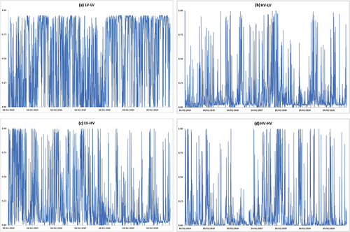
Table 6. Comparative analysis of various volatility states.

	BTC = LV and Other = LV	BTC = HV and Other = LV	BTC = LV and Other = HV	BTC = HV and Other = HV
Panel A. Observation percentages of various volatility combination states
BTC-DASH	57.48%	9.65%	21.69%	11.19%
BTC-LIT	65.14%	11.27%	13.01%	10.58%
BTC-XRP	56.91%	16.94%	14.80%	11.35%
Panel B. Risk reduction effectiveness of diversification in various volatility states
BTC-DASH	6.50%	17.49%	13.25%	2.39%
BTC-LIT	15.63%	23.96%	13.94%	6.67%
BTC-XRP	7.26%	16.47%	12.66%	6.63%

On key feature of the bivariate SWARCH model is to provide the estimated probabilities of a specific state for each point in time (the BTC-DASH example is shown in Figure 4). We use these estimated probabilities and a maximum value criterion to define the volatility state. For example, if the estimated probability of the ‘HV-HV’ state is higher than that of the other three states, we identify this point in time as an ‘HV-HV’ state.

In panel B, we show the risk reduction percentage of a cryptocurrency portfolio with equal weight on each cryptocurrency. More specifically, the risk reduction percentage of a cryptocurrency portfolio is presented as follows.

Risk reduction % = −100*[σ_p - (0.5 × σ^BTC +0.5 × σ^OTH)]/(0.5 × σ^BTC +0.5 × σ^OTH)

where σ^BTC and σ^OTH denote the standard deviation of Bitcoin and another cryptocurrency in the portfolio, respectively. The σ_p is the standard deviation of the cryptocurrency portfolio with equal weight on Bitcoin and another cryptocurrency. The figure in bold style represents the minimum value in the row.

Next, we develop the measure of the reduction percentage of a portfolio as follows:

(16) $\begin{array}{rl}& \mathrm{R}\mathrm{i}\mathrm{s}\mathrm{k}\mathrm{r}\mathrm{e}\mathrm{d}\mathrm{u}\mathrm{c}\mathrm{t}\mathrm{i}\mathrm{o}\mathrm{n}\mathrm{\%}=\\ & -100\ast \left[{\sigma }_{\mathrm{p}}-\left(0.5\times {\sigma }^{\mathrm{B}\mathrm{T}\mathrm{C}}+0.5\times {\sigma }^{\mathrm{O}\mathrm{T}\mathrm{H}}\right)\right]/\left(0.5\times {\sigma }^{\mathrm{B}\mathrm{T}\mathrm{C}}+0.5\times {\sigma }^{\mathrm{O}\mathrm{T}\mathrm{H}}\right)\end{array}$(16)

where the σ^BTC and σ^OTH denote the standard deviation of BTC and OTH returns, respectively. The σ^p is the standard deviation of the cryptocurrency portfolio return with equal weight on BTC and OTH digital currencies, that is, r_t^p = r_t^BTC + r_t^OTH. A higher/lower value of risk reduction percentage implies the greater/lesser effectiveness of portfolio risk diversification.

The results, presented in Panel B of Table 6, indicate that the ‘HV-HV’ volatility state corresponds to the minimum value of risk reduction effectiveness in all the cases. Using the BTC-DASH portfolio as an example, the risk reduction % at the ‘HV-HV’ state is 2.39% and the risk reduction % for the other three states ranges from 6.50% to 17.49%. These findings have implications for cryptocurrency investment risk management. First, risk management is critical and important in a high-volatility situation. Unfortunately, under the ‘HV-HV’ situation, portfolio diversification in digital currency markets corresponds to the least effectiveness in risk reduction. This result echoes our aforementioned findings in Table 5: a strong correlation in the digital currency markets under the ‘HV-HV’ state, that is, ρ_2,2.

Based on our framework, the correlation is expected to be generally weak when the paired cryptocurrencies are experiencing an opposite volatility regime, namely, one in an HV state and the other in an LV state. Further, the co-movement becomes much stronger when the paired cryptocurrencies face an identical volatility regime, that is, both are experiencing an HV or LV volatility state (see Section 2.2). Experiencing an identical volatility condition in the paired digital currency markets is related to co-jumping behaviours in the literature. We thus link co-jumping behaviours with correlation dynamics between various cryptocurrencies. As shown in Panel A of Table 6, the observation percentages of an identical volatility regime (i.e. LV-LV plus HV-HV) are higher than the value of an opposite volatility regime (i.e. HV-LV plus LV-HV). Using the BTC-DASH pair as an example, the observation percentage of an identical volatility regime is 68.67% ( = 57.48% + 11.10%), and the observation percentage of an opposite volatility regime is 31.33% ( = 9.65% + 21.68%). This result supports co-jumping behaviours in cryptocurrency markets. Moreover, as shown in Table 5, the magnitude of the estimates of ρ_2,2 and ρ_1,1 is considerably higher than those calculated for the other two possible state groupings: ρ_2,1 and ρ_1,2.

5.2. Cryptocurrency portfolio risk forecasting

This section conducts the second practical test for digital currency investment risk management: portfolio risk forecasting. As previously stated, the risk of a portfolio hinges on asset volatilities and their correlations. This study employs three alternative empirical models on the data of cryptocurrencies, including the two bivariate GARCH models and the bivariate SWARCH model. We seek to determine whether our bivariate SWARCH model with state-dependent variances and correlations is more effective in predicting the risk of the cryptocurrency portfolios than the conventional GARCH models with simple time-dependent variances and correlations.

MAE (Mean Absolute Error) and MSE (Mean Square Error), the two most prominent forecasting performance measures, are adopted and the results are presented in Table 7. It should be noted that four separate volatility state groupings are defined in our bivariate SWARCH model. We compute the weighted average of portfolio risk according to the estimated probabilities of volatility states. In particular, we first compute the portfolio risks under various volatility state combinations (i.e. LV-LV, HV-LV, LV-HV and HV-HV). Then the probabilities of each specific volatility state combination are used as the weights to compute the weighted average (see Figure 2: An example of the BTC-DASH portfolio).

Table 7. Cryptocurrency portfolio volatility forecasting.

	BTC-DASH	BTC-LTC	BTC-XRP
Panel A: MAE (Mean Absolute Error)
Bivariate GARCH-CCC model	5.6735	5.5252	5.3308
Bivariate GARCH-DCC model	5.8192	5.6514	5.3778
Bivariate SWARCH model	4.9442 (−5.4657)***	4.4683 (−8.9052)***	4.2007 (−8.7868)***
Panel B: MSE (Mean Square Error)
Bivariate GARCH-CCC model	57.5218	49.7362	52.3870
Bivariate GARCH-DCC model	61.8947	52.6608	53.8310
Bivariate SWARCH model	43.0255 (−2.8237)***	35.4926 (−3.0311)***	34.4661 (−3.1250)***

This study adopts MSE and MAE, the two commonly-used forecasting performance criteria, to evaluate the performance of various models in cryptocurrency portfolio volatility forecasting. The MSE and MAE are defined as follows.

$MSE=T^{-1}\sum _{t=1}^T{\left(r_{p,t}^2-{\sigma }_{p,t}^2\right)}^2$, $MAE=T^{-1}\sum _{t=1}^T\left|r_{p,t}^2-{\sigma }_{p,t}^2\right|$.

where r_p,t is the portfolio return with equal weight on each digital currency and σ_p,t is the estimated standard deviation of the digital currency portfolio. The figure in bold style represents the minimum value in the column. As shown in the table, the bivariate SWARCH model associates with the smallest MSE and MAE.

We adopt the bivariate GARCH-CCC model as a benchmark and calculate the statistic for the difference in MSE and MAE (see the figure in parenthesis). *** represents significance at the 1% level.

As shown in Table 7, the bivariate SWARCH model, equipped with state-dependent variances and correlations, offers an advantage over the bivariate GARCH model with simple time-dependent variances and correlations in terms of risk forecasting performance. Specifically, the bivariate SWARCH model associates with the smallest MSE and MAE. Next, the bivariate GARCH model with a constant conditional correlation (i.e. the GARCH-CCC model) is adopted as a benchmark to calculate the statistic of the difference in MSE and MAE. The difference is significant at 1% for all three cryptocurrency portfolios. Our conclusion is clear: designing a model to capture volatility regimes and correlation dynamics in the digital currency markets (i.e. the bivariate SWARCH model in this study) can produce a better estimate of digital currency portfolio risk than the use of conventional GARCH-based models.

5.3. Cryptocurrency portfolio construction

In this section, we proceed with the third practical test regarding cryptocurrency investment risk: portfolio construction. As is well known, portfolio construction relies on the quality of variance and correlation estimation. Accordingly, an important question is whether the state-varying variances and correlations addressed in this study may help an investor develop a more efficient cryptocurrency portfolio. Since our focus is cryptocurrency investment risk, we adopt a minimum variance portfolio construction strategy to conduct this test (e.g. French and Poterba 1991; Tesar and Werner 1992; Ramchand and Susmel 1998). Considering the BTC-OTH portfolio, the weight given to each cryptocurrency asset is presented as follows:

(17) $\begin{array}{rl}& w_t^{BTC}=\\ & \left[h_t^{OTH}-{\rho }_t{\left(h_t^{OTH}\cdot h_t^{BTC}\right)}^{1/2}\left]/\right[h_t^{BTC}+h_t^{OTH}-2\cdot {\rho }_t{\left(h_t^{OTH}\cdot h_t^{BTC}\right)}^{1/2}\right]\end{array}$(17)

(18) $w_t^{OTH}=1-w_t^{BTC}$(18)

where w_t^BTC and w_t^OTH represent the weight given to BTC (Bitcoin) and OTH (OTH denotes the other digital currency in the portfolio, namely, DASH, LIT or XRP), respectively. h_t^BTC and h_t^OTH denote the conditional variances of BTC and OTH respectively and ρ_t is the correlation between them.

Given the weights, we then calculate the return of the BTC-OTH portfolio at each point in time ($r_t^{POT}$):

(19) $r_t^{POT}=w_t^{BTC}\cdot r_t^{BTC}+w_t^{OTH}\cdot r_t^{OTH}$(19)

Next, we calculate the volatility of the BTC-OTH portfolio return over the testing period and examine whether the volatility varies significantly between the bivariate GARCH (a pure time-varying approach) and SWARCH (a state-varying approach) models.

Table 8 show the performance of portfolio construction by various models, including the bivariate GARCH-CCC, GARCH-DCC and SWARCH. Restated, the focus of this study is the risk of cryptocurrency investment. We thus concentrate on the paired cryptocurrency portfolios’ volatility (i.e. standard deviation). As shown in Table 8, the portfolio’s volatility constructed by the bivariate SWARCH model is lower than that of the two bivariate GARCH models. Moreover, when we use the bivariate GARCH-CCC portfolio as a benchmark, the risk reduction of the cryptocurrency portfolio constructed by the bivariate SWARCH model is significant at a 1% level. Our conclusion is clear: modelling variances of cryptocurrencies and their correlations using a regime-switching system improves the performance of cryptocurrency portfolio construction.¹²

Table 8. Portfolio construction performance: Volatility of cryptocurrency portfolio.

	BTC-DASH	BTC-LTC	BTC-XRP
Bivariate GARCH-CCC model	3.8397	3.9954	3.7064
Bivariate GARCH-DCC model	3.8159 (−1.4785)	4.0017 (0.5044)	3.7102 (0.1925)
Bivariate SWARCH model	3.4359 (−10.1508)***	3.4736 (−4.8288)***	3.1974 (−6.7017)***

This table lists the performance of portfolio construction between various models. As our focus is risk of cryptocurrency investment, we adopt a minimum variance portfolio strategy to test the issue and present the volatility (standard deviation) of the cryptocurrency portfolios in this table (e.g. French and Poterba 1991; Tesar and Werner 1992; Ramchand and Susmel 1998).

The figure in bold style represents the minimum value in the column. We use the bivariate GARCH-CCC model as a benchmark to calculate the statistic for the difference in the portfolio volatility (see the figure in the parenthesis). *** represents significance at the 1% level.

6. Conclusions and future research directions

The exponential growth of attention to the cryptocurrency markets reflects their tremendous investment returns. However, these markets are characterized by a lack of regulations and are volatile. Therefore, measuring and managing the risk of cryptocurrency investment is essential. In this study, the risk of trading on cryptocurrencies is measured by their second moments, that is, variances and correlations. We break new ground by addressing the phenomenon of volatility regimes and examining their relationship with correlations in the digital currency markets. We build on this work by developing a theoretical hypothesis for these phenomena in the digital currency markets. We also employ a bivariate SWARCH model involved with the regime-switching variances and correlations to test our hypothesis.

Our novel approach identifies various volatility regimes in the cryptocurrency markets and analyzes their correlation dynamics under different volatility regimes. While existing studies have tested the dynamics of correlations in the digital currency markets (the majority of the studies use the conventional GARCH and DCC models), none have explicitly addressed correlation dynamics under various volatility regimes. This initial study fills this gap in the literature and offers several contributions, including the use of a specific econometric method and providing three practical tests for cryptocurrency risk management. The three practical tests are meaningful in the practical field and thus help to bring the statistical estimation results nearer to practical. We employ four representative cryptocurrencies – Bitcoin (BTC), Dash (DASH), Litecoin (LTC) and Ripple (XRP) – to conduct the empirical tests. Our sample period is between 14 February 2014 and 19 November 2020 for 2,471 daily observations.

Our empirical findings are consistent with the following notions. First, volatility regimes display in the digital currency markets and serve as a determinant of the cross-market correlations. In particular, the correlation between the paired digital currency markets is stronger when they are in the same state of volatility (i.e. HV-HV and LV-LV) whereas their correlation is weaker when they are in an opposite state of volatility (i.e. LV-HV and HV-LV). Second, the circumstance in which both the paired digital currency markets are simultaneously encountering a high volatility regime (i.e. HV-HV) is associated with the least effectiveness of portfolio risk diversification. Our findings echo co-jumping behaviours addressed by the digital currency market literature. Last but not least, the bivariate SWARCH model, with its state-dependent variances and correlations, significantly outperforms the conventional GARCH and DCC models with their simple time-dependent variances and correlations in terms of cryptocurrency portfolio risk forecasting and portfolio construction.

Lastly, we note two limitations of this study and address future research directions. First, further development of the programme codes for this general model based on a general 4 × 4 transition probability matrix (see the Appendix section) is worthy of future research. Second, the in-sample performances, as in Tables 7 and 8, show the historical performance of the competitive models. Future researchers may further conduct out-of-sample tests.

Disclosure statement

No potential conflict of interest was reported by the author(s).

Data availability statement

https://coinmarketcap.com/

Notes

¹ See Alexander Osipovich and Eun-Young Jeong, the Wall Street Journal: https://www.wsj.com/articles/bitcoins-crashing-that-wont-stop-arbitrage-traders-from-raking-in-millions-1517749201.

² The literature on cryptocurrencies point out several factors that might influence the prices of digital currencies, such as monetary policy (Kristoufek and Scalas 2015), financial regulations (Pieters and Vivanco 2017), economic variables (Zhu, Dickinson, and Li 2017), and media coverage (Glaser et al. 2014).

³ Some studies examine whether cryptocurrencies may act as a safe-haven asset in mitigating the risk of stock positions (e.g. Bouri et al. 2017; Garcia-Jorcanoa and Benito 2020; Mariana, Ekaputra, and Husodo 2021; Huang et al. 2022).

⁴ A few recent studies, including Kang, McIver, and Hernandez (2019), Pavković, Anđelinović, and Pavković (2019), Kumar and Anandarao (2019), Kumar and Ajaz (2019), Mensi et al. (2020), employ the wavelet correlation techniques (nonparametric methods) to examine the correlations among the digital currency markets. Frankovic, Liu, and Suardi (2021) use the spillover index proposed by Diebold and Yilmaz (2012) to test the correlation between the Australian listed cryptocurrency-linked stocks and cryptocurrency markets.

⁵ The first step of this approach is to run the univariate GARCH model for each asset (cryptocurrencies in this study). The second step is to run the DCC model using the residual of the univariate asset. As such, the estimation of correlations is assumed to be independent with the estimation of variances.

⁶ Bouri, Roubaud, and Shahzad (2020) analyse jumps in the mean. Meanwhile, Gkillas et al. (2022) analyse the co-jumping behaviour, that is, the effects of a cryptocurrency volatility jump on the volatility jumps of the other cryptocurrency.

⁷ See Bollerslev (1990) and Baillie and Bollerslev (1990).

⁸ Our DCC model in Equations (8) and (9) is not exactly the same as Engle’s (2002). The Q_t term in Engle’s paper is the covariance matrix, while we follow his paper to develop the dynamic conditional correlations. For the correlation matrix, the diagonal elements are unity, ranging from −1.0 to 1.0. Equation (9)(9) ${\rho }_t=q_t/\sqrt{1+q_t^2}$(9) is thus developed to control the magnitude of the correlation coefficient within this theoretical range. The difference between our Equation (8)(8) $q_t=\tau +\pi \cdot q_{t-1}+\lambda \cdot e_{t-1}^{BTC}\cdot e_{t-1}^{OTH}/\sqrt{h_{t-1}^{BTC}\cdot h_{t-1}^{OTH}}$(8) and Engle’s Equation (23) is that the former simply shows the DCC for the bivariate data (i.e. the portfolio with two assets), and the latter uses the correlation matrix to show the DCC setting for the multivariate data (i.e. the portfolio with n assets). We thank the reviewer for the clarification of this point.

⁹ In this study, all the model parameters (including variances and correlations) are estimated using a one-step process. This one-step estimation process may effectively mitigate the limitation of independence assumption in a two-step estimation process.

¹⁰ The price levels of the four selected cryptocurrencies are unable to reject I(1). This result reveals that they are a non-stationary time series. Next, we examine the results of the return rates on cryptocurrencies. Overall, the presence of unit root (i.e. I(1) time series), is rejected, implying that the return rates on cryptocurrencies are a stationary time series. The unit-root test results are available on request.

¹¹ As shown in Table 4, the sum of the two estimates for GARCH volatilities and the two estimates for the DCC model is close to 1. Diebold (1986) and Lamoureux and Lastrapes (1990) point out that the high persistence of volatilities is caused by the structural changes in the volatility process during the estimation period. Our empirical results of the DCC models further show the high persistence of correlations. These findings support the implementation of regime-switching techniques into conditional volatilities and correlations.

¹² In addition to portfolio risk, we also calculate portfolio return constructed by various models (not tabulated). However, the difference in portfolio return between the bivariate GARCH and SWARCH models is insignificant. This result implies that reductions in risk, rather than increases in return mean, are to be thanked for the benefits stemming from such improved performance.

Appendix

Appendix: A four-state regime-switching system

This study develops a bivariate SWARCH model to capture regime-switching conditional correlations, and considers relations with conditional variances. Based on this system thus described, the construction of the latent variable s_t on the basis of the separate latent processes s_t^BTC and s_t^OTH can be visually depicted as follows:

s_t = 1: if s_t^BTC = 1 and s_t^OTH = 1 -or- BTC = LV and the other cryptocurrency = LV

s_t = 2: if s_t^BTC = 2 and s_t^OTH = 1 -or- BTC = HV and the other cryptocurrency = LV

s_t = 3: if s_t^BTC = 1 and s_t^OTH = 2 -or- BTC = LV and the other cryptocurrency = HV

s_t = 4: if s_t^BTC = 2 and s_t^OTH = 2 -or- BTC = LV and the other cryptocurrency = HV

As was assumed in the case of the univariate analysis, s_t is an unobservable state variable and is associated with possible outcomes of 1, 2, 3 and 4. Furthermore, this state variable is held to follow a first-order 4-state Markov chain model formulated as follows:

(A1) $P\left(s_t^{\hspace{0.17em}}=j|s_{t-1}^{\hspace{0.17em}}=i\right)=p_{ij}^{\hspace{0.17em}}$(A1)

Thus, the 4 × 4 transition probability matrix of this model can be depicted below:

(A2) $P=\left[\begin{array}{cccc}{p}_{11}& p_{21}& p_{31}& p_{41}\\ p_{12}& p_{22}& p_{32}& p_{42}\\ p_{13}& p_{23}& p_{33}& p_{43}\\ p_{14}& p_{24}& p_{34}& p_{44}\end{array}\right]$(A2)

In our study, we assume the variance-switching process of each cryptocurrency in the pair is here seen as subject to the distinct processes of switching volatility states characterizing each market component. Therefore, we have a 2 × 2 transition probability matrix for each cryptocurrency in the pair:

$P^{BTC}=\hspace{0.17em}\left[\begin{array}{ccc}{p}_{11}^{BTC}& & p_{21}^{BTC}\\ p_{12}^{BTC}& p_{22}^{BTC}\end{array}\right]$ and $P^{OTH}=\hspace{0.17em}\left[\begin{array}{cc}{p}_{11}^{OTH}& p_{21}^{OTH}\\ p_{12}^{OTH}& p_{22}^{OTH}\end{array}\right]$ (A3)

Notably, we may use these two 2 × 2 transition matrices to generate the 4 × 4 transition probability matrix:

(A4) $p=\left[\begin{array}{c}{p}_{11}^{BTC}\times p_{11}^{OTH}\times p_{21}^{BTC}\times p_{11}^{OTH}\times p_{11}^{BTC}\times p_{21}^{OTH}\times p_{21}^{BTC}\times p_{21}^{OTH}\\ p_{12}^{BTC}\times p_{11}^{OTH}\times p_{22}^{BTC}\times p_{11}^{OTH}\times p_{12}^{BTC}\times p_{21}^{OTH}\times p_{22}^{BTC}\times p_{21}^{OTH}\\ p_{11}^{BTC}\times p_{12}^{OTH}\times p_{21}^{BTC}\times p_{12}^{OTH}\times p_{11}^{BTC}\times p_{22}^{OTH}\times p_{21}^{BTC}\times p_{22}^{OTH}\\ p_{12}^{BTC}\times p_{12}^{OTH}\times p_{22}^{BTC}\times p_{12}^{OTH}\times p_{12}^{BTC}\times p_{22}^{OTH}\times p_{22}^{BTC}\times p_{22}^{OTH}\end{array}\right]$(A4)

Using the BTC-DASH pair as an illustrative example, we calculate its 4 × 4 transition probability matrix as follows:

(A5) $P=\left[\begin{array}{cccc}0.8321& 0.2180& 0.1372& 0.0359\\ 0.0785& 0.6926& 0.0129& 0.1142\\ 0.0817& 0.0214& 0.7766& 0.2045\\ 0.0077& 0/0680& 0.0733& 0.6464\end{array}\right]$(A5)

A comparison of the two ostensibly identical four-state switching models depicted in Equations (A2(A2) $P=\left[\begin{array}{cccc}{p}_{11}& p_{21}& p_{31}& p_{41}\\ p_{12}& p_{22}& p_{32}& p_{42}\\ p_{13}& p_{23}& p_{33}& p_{43}\\ p_{14}& p_{24}& p_{34}& p_{44}\end{array}\right]$(A2) ) and eq(A3) reveals significant differences in the number of population parameters required to estimate. In the case of the general model presented in Equation (A2)(A2) $P=\left[\begin{array}{cccc}{p}_{11}& p_{21}& p_{31}& p_{41}\\ p_{12}& p_{22}& p_{32}& p_{42}\\ p_{13}& p_{23}& p_{33}& p_{43}\\ p_{14}& p_{24}& p_{34}& p_{44}\end{array}\right]$(A2) , s_t follows a four-state Markov chain, the transition matrix of which is restricted by the condition that each column must sum to unity, hence the need for 12 probability parameters. On the other hand, the estimation of only 4 ( = 2 + 2) probability parameters is required in the restricted four-state model presented in Equation (A3).

References

- Aielli, G. P. 2013. “Dynamic Conditional Correlation: On Properties and Estimation.” Journal of Business and Economic Statistics 31 (3): 282–299. doi:10.1080/07350015.2013.771027.
- Antonis, B., and D. Konstantinos. 2019. “Testing for Herding in the Cryptocurrency Market.” Finance Research Letters in Press 33: 101210. doi:10.1016/j.frl.2019.06.008.
- Aslanidis, N., A. F. Bariviera, and O. Martínez-Ibañez. 2019. “An Analysis of Cryptocurrencies Conditional Cross Correlations.” Finance Research Letters 31: 130–137. doi:10.1016/j.frl.2019.04.019.
- Baillie, R. T., and T. Bollerslev. 1990. “A Multivariate Generalized ARCH Approach to Modeling Risk Premia in Forward Foreign Exchange Rate Markets.” Journal of International Money and Finance 9 (3): 309–324. doi:10.1016/0261-5606(90)90012-O.
- Bollerslev, T. 1990. “Modelling the Coherence in Short-Run Nominal Exchange Rates: A Multivariate Generalized ARCH Model.” The Review of Economics and Statistics 72 (3): 498–505. doi:10.2307/2109358.
- Bouri, E., R. Gupta, A. Tiwari, and D. Roubaud. 2017. “Does Bitcoin Hedge Global Uncertainty? Evidence from Wavelet-Based Quantile-In-Quantile Regressions.” Finance Research Letters 23: 87–95. doi:10.1016/j.frl.2017.02.009.
- Bouri, E., D. Roubaud, and S. J. H. Shahzad. 2020. “Do Bitcoin and Other Cryptocurrencies Jump Together?” The Quarterly Review of Economics and Finance 76: 396–409. doi:10.1016/j.qref.2019.09.003.
- Bouri, E., X. V. Vo, and T. Saeed. 2021. “Return Equicorrelation in the Cryptocurrency Market: Analysis and Determinants.” Finance Research Letters 38: 101497. doi:10.1016/j.frl.2020.101497.
- Cheah, E. T., and J. Fry. 2015. “Speculative Bubbles in Bitcoin Markets? An Empirical Investigation into the Fundamental Value of Bitcoin.” Economics Letters 130: 32–36. doi:10.1016/j.econlet.2015.02.029.
- Chen, C., and C. M. Hafner. 2019. “Sentiment-Induced Bubbles in the Cryptocurrency Market.” Journal of Risk and Financial Management 12 (2): 53. doi:https://doi.org/10.3390/jrfm12020053.
- Diebold, F. X. 1986. “Modeling the Persistence of Conditional Variance: A Comment.” Econometric Reviews 5 (1): 51–56. doi:10.1080/07474938608800096.
- Diebold, F. X., and K. Yilmaz. 2012. “Better to Give Than to Receive: Predictive Directional Measurement of Volatility Spillovers.” International Journal of Forecasting 28 (1): 57–66. doi:10.1016/j.ijforecast.2011.02.006.
- Engle, R. F. 2002. “Dynamic Conditional Correlation: A Simple Class of Multivariate Generalized Autoregressive Conditional Heteroskedasticity Models.” Journal of Business and Economic Statistics 20 (3): 339–350. doi:10.1198/073500102288618487.
- Frankovic, J., B. Liu, and S. Suardi. 2021. “On Spillover Effects Between Cryptocurrency-Linked Stocks and the Cryptocurrency Market: Evidence from Australia.” Global Finance Journal in Press 54: 100642. doi:10.1016/j.gfj.2021.100642.
- French, K. R., and J. M. Poterba. 1991. “Investor Diversification and International Equity Markets.” The American Economic Review 81: 222–226.
- Fry, J., and E. T. Cheah. 2016. “Negative Bubbles and Shocks in Cryptocurrency Markets.” International Review of Financial Analysis 47: 343–352. doi:10.1016/j.irfa.2016.02.008.
- Fung, K., J. Jeong, and J. Pereira. 2022. “More to Cryptos Than Bitcoin: A GARCH Modelling of Heterogeneous Cryptocurrencies.” Finance Research Letters 47: 102544. doi:10.1016/j.frl.2021.102544.
- Garcia-Jorcanoa, L., and S. Benito. 2020. “Studying the Properties of the Bitcoin as a Diversifying and Hedging Asset Through a Copula Analysis: Constant and Time-Varying.” Research in International Business and Finance 54: 101300. doi:10.1016/j.ribaf.2020.101300.
- Gkillas, K., P. Katsiampa, C. Konstantatos, and A. Tsagkanos. 2022. “Discontinuous Movements and Asymmetries in Cryptocurrency Markets.” Resource Policy 1–25. doi:10.1080/1351847X.2021.2015416).
- Glaser, F., K. Zimmermann, M. Haferkorn, M. C. Weber, and M. Siering 2014 Bitcoin-Asset or Currency? Revealing Users’ Hidden Intentions, Working paper, Available at SSRN: https://ssrn.com/abstract=2425247.
- Godsiff, P. 2015. “Bitcoin: Bubble or Blockchain, Agent and Multi-Agent Systems.” Technologies and Applications 38: 191–203.
- Hasan, M. B., M. K. Hassan, M. M. Rashid, and Y. Alhenawi. 2021. “Are Safe Haven Assets Really Safe During the 2008 Global Financial Crisis and COVID-19 Pandemic?” Global Finance Journal in Press 50: 100668. doi:10.1016/j.gfj.2021.100668.
- Huang, X., W. Han, D. Newton, E. Platanakis, D. Stafylas, and C. Sutcliffe. 2022. “The Diversification Benefits of Cryptocurrency Asset Categories and Estimation Risk: Pre and Post Covid-19.” The European Journal of Finance in Press 1–26. doi:10.1080/1351847X.2022.2033806.
- Kang, S. H., R. P. McIver, and J. A. Hernandez. 2019. “Co-Movements Between Bitcoin and Gold: A Wavelet Coherence Analysis, Physica A: Statistical Mechanics and Its Applications 536.” Physica A: Statistical Mechanics and Its Applications 536: 120888. doi:https://doi.org/10.1016/j.physa.2019.04.124.
- Katsiampa, P. 2019. “Volatility Co-Movement Between Bitcoin and Ether.” Finance Research Letters 30: 221–227. doi:10.1016/j.frl.2018.10.005.
- Katsiampa, P., S. Corbet, and B. Lucey. 2019. “High Frequency Volatility Co-Movements in Cryptocurrency Markets.” Journal of International Financial Markets, Institutions and Money 62: 35–52. doi:10.1016/j.intfin.2019.05.003.
- King, M. A., and S. Wadhwani. 1990. “Transmission of Volatility Between Stock Markets.” The Review of Financial Studies 3 (1): 5–33. doi:10.1093/rfs/3.1.5.
- Kostika, E., and N. T. Laopodis. 2019. “Dynamic Linkages Among Cryptocurrencies, Exchange Rates and Global Equity Markets.” Studies in Economics and Finance 37 (2): 243–265. doi:10.1108/SEF-01-2019-0032.
- KPMG 2022. Canadian institutional investors are growing their crypto asset holdings. April 6, 2022. Downloaded fromhttps://home.kpmg/ca/en/home/media/press-releases/2022/04/canadian-investors-adding-crypto-to-their-portfolios.html.
- Kristoufek, L., and E. Scalas. 2015. “What are the Main Drivers of the Bitcoin Price? Evidence from Wavelet Coherence Analysis.” Plos One 10 (4): 1–15. doi:10.1371/journal.pone.0123923.
- Kumar, A. S., and T. Ajaz. 2019. “Co-Movement in Crypto-Currency Markets: Evidences from Wavelet Analysis.” Financial Innovation 5 (1). doi:https://doi.org/10.1186/s40854-019-0143-3.
- Kumar, A. S., and S. Anandarao. 2019. “Volatility Spillover in Crypto-Currency Markets: Some Evidences from GARCH and Wavelet Analysis.” Physica A: Statistical Mechanics and Its Applications 524: 448–458. doi:10.1016/j.physa.2019.04.154.
- Lamoureux, C. G., and W. D. Lastrapes. 1990. “Persistence in Variance, Structural Change and the GARCH Model.” Journal of Business and Economic Statistics 8 (2): 225–234. doi:10.1080/07350015.1990.10509794.
- Li, L. 2022. “The Dynamic Interrelations of Oil-Equity Implied Volatility Indexes Under Low and High Volatility-Of-Volatility Risk.” Energy Economics 105: 105756.
- Lyócsa, Š., P. Molnár, T. Plíhal, and M. Širaňová. 2020. “Impact of Macroeconomic News, Regulation and Hacking Exchange Markets on the Volatility of Bitcoin.” Journal of Economic Dynamics & Control 119: 103980. doi:10.1016/j.jedc.2020.103980.
- Maciel, L. 2021. “Cryptocurrencies Value-At-Risk and Expected Shortfall: Do Regime-Switching Volatility Models Improve Forecasting?” International Journal of Finance & Economics 26 (3): 4840–4855. doi:10.1002/ijfe.2043.
- Mariana, C. D., I. A. Ekaputra, and Z. A. Husodo. 2021. “Are Bitcoin and Ethereum Safe-Havens for Stocks During the COVID-19 Pandemic?” Finance Research Letters 38: 101798. doi:10.1016/j.frl.2020.101798.
- Markowitz, H. M. 1991. “Foundations of Portfolio Theory.” The Journal of Finance 46 (2): 469–477. doi:10.1111/j.1540-6261.1991.tb02669.x.
- Mensi, W., M. U. Rehman, K. H. Al-Yahyaee, I. M. W. Al-Jarrah, and S. H. Kang. 2019. “Time Frequency Analysis of the Commonalities Between Bitcoin and Major Cryptocurrencies: Portfolio Risk Management Implications.” The North American Journal of Economics and Finance 48: 283–294. doi:10.1016/j.najef.2019.02.013.
- Mensi, W., M. U. Rehman, D. Maitra, K. H. Al-Yahyaee, and A. Sensoy. 2020. “Does Bitcoin Co-Move and Share Risk with Sukuk and World and Regional Islamic Stock Markets? Evidence Using a Time-Frequency Approach.” Research in International Business and Finance 53: 101230. doi:10.1016/j.ribaf.2020.101230.
- Nadarajah, S., and J. Chu. 2017. “On the Inefficiency of Bitcoin.” Economics Letters 150: 6–9. doi:10.1016/j.econlet.2016.10.033.
- Neureuter, J. 2021. The Institutional Investor Digital Assets Study. September 2021 fromFidelity Digital Assets Downloaded https://www.fidelitydigitalassets.com/sites/default/files/documents/2021-digital-asset-study_0.pdf.
- Park, Y. K., K. B. Binh, and S. J. Kim. 2019. “Time Varying Correlations and Causalities Between Stock and Foreign Exchange Markets: Evidence from China, Japan and Korea.” Investment Analysts Journal 48 (4): 278–297. doi:10.1080/10293523.2019.1670385.
- Pavković, A., M. Anđelinović, and I. Pavković. 2019. “Achieving Portfolio Diversification Through Cryptocurrencies in European Markets.” Business Systems Research Journal 10 (2): 85–107. doi:10.2478/bsrj-2019-020.
- Perrin, A. 2021. 16% of Americans Say They Have Ever Invested In, Traded or Used Cryptocurrency. November 11, 2021. Pew Research Center. Downloaded from https://www.pewresearch.org/fact-tank/2021/11/11/16-of-americans-say-they-have-ever-invested-in-traded-or-used-cryptocurrency/.
- Pieters, G., and S. Vivanco. 2017. “Financial Regulations and Price Inconsistencies Across Bitcoin Markets.” Information Economics and Policy 39: 1–14. doi:10.1016/j.infoecopol.2017.02.002.
- Ramchand, L., and R. Susmel. 1998. “Volatility and Cross Correlation Across Major Stock Markets.” Journal of Empirical Finance 5 (4): 397–416. doi:10.1016/S0927-5398(98)00003-6.
- Salisua, A. A., and A. E. Ogbonna. 2021. “The Return Volatility of Cryptocurrencies During the COVID-19 Pandemic: Assessing the News Effect.” Global Finance Journal in Press 54: 100641. doi:10.1016/j.gfj.2021.100641.
- Scaillet, O., A. Treccani, and C. Trevisan. 2020. “High-Frequency Jump Analysis of the Bitcoin Market.” Journal of Financial Econometrics 18: 209–232.
- Siu, T. K., and R. J. Elliott. 2021. “Bitcoin Option Pricing with a SETAR-GARCH Model.” The European Journal of Finance 27 (6): 6, 564–595. doi:10.1080/1351847X.2020.1828962.
- Stefano, B., C. Alessandra, F. T. Gianna, and P. Marco. 2019. “Model-Based Arbitrage in Multi-Exchange Models for Bitcoin Price Dynamics.” Digital Finance 1 (1–4): 23–46. doi:10.1007/s42521-019-00001-2.
- Tesar, L. L., and I. Werner 1992 Home Bias and the Globalization of Securities Markets, NBER Working Paper, No. 4218, National Bureau of Economic Research, Cambridge.
- Tiwari, A. K., S. Kumar, and R. Pathak. 2019. “Modelling the Dynamics of Bitcoin and Litecoin: GARCH versus Stochastic Volatility Models.” Applied Economics 51 (37): 4073–4082. doi:10.1080/00036846.2019.1588951.
- Todorov, V., and G. Tauchen. 2011. “Volatility Jumps.” Journal of Business and Economic Statistics 29 (3): 356–371. doi:10.1198/jbes.2010.08342.
- Trevino, I. 2020. “Informational Channels of Financial Contagion.” Econometrica 88 (1): 297–335. doi:10.3982/ECTA15604.
- Urquhart, A. 2016. “The Inefficiency of Bitcoin.” Economics Letters 148: 80–82. doi:10.1016/j.econlet.2016.09.019.
- Zhu, Y., D. Dickinson, and J. Li. 2017. “Analysis on the Influence Factors of Bitcoin’s Price Based on VEC Model.” Financial Innovation 3 (1): 1–13. doi:10.1186/s40854-017-0054-0.