Physical infrastructure and economic growth

ABSTRACT

The existing literature on the relationship between infrastructure and economic growth is inconclusive. We estimate the effect on GDP of three main categories of infrastructure – transport, electricity, and telecommunications – using data from 87 countries over the period 1992–2017. This study uses more recent data than previous research and includes new types of infrastructure such as mobile phones. Our main estimates use the PMG estimator that allows us to test for the weak exogeneity of the infrastructure variables. The key finding of the study is that an increase in infrastructure, especially electricity generation capacity and telecommunications, has large long-run positive effects on GDP, though the short-run effects are much smaller and are less than zero for roads and railways. Also, the effects of electricity and communication infrastructure are higher relative to the effects of transport infrastructure in developing economies than in industrialized economies.

KEYWORDS:

• Infrastructure
• growth
• mobile phones
• pooled mean group estimator

JEL CLASSIFICATION:

• O18
• O47

I. Introduction

Policymakers, particularly in developing countries, often face a critical question: how much they should invest in physical infrastructure from their scarce financial resources, both resources generated domestically and provided by foreign sources such as bilateral and multilateral donors and direct foreign investment. This question is also important for international development institutions such as the World Bank Group’s regional development banks who wish to maximize their impact on economic development and social welfare in recipient economies.

Timilsina, Hochman, and Song (2020) review a large body of literature and conclude that no consensus exists on the impacts of infrastructure investment on economic growth. Some existing studies show a strong positive relationship between infrastructure development and economic growth, whereas others find a mildly positive relationship or no relationship. Many factors are responsible for these varying results, such as differences in methods, differing approaches to measuring infrastructure development, the varying development stages of countries included in the sample, varying time periods, and geographical factors such as high or low population density (Timilsina, Hochman, and Song 2020; Elburz, Nijkamp, and Pels 2017¹).

To further illuminate the role of infrastructure in economic growth and development, this study uses a dynamic panel data model to evaluate the contributions of three main categories of infrastructure: transport, electricity, and telecommunications, to growth in a panel of 87 countries over the period 1992 to 2017. We use the pooled mean group estimator (Pesaran, Shin, and Smith 1999) to estimate the effects of these and other inputs on growth.

The best previous research on this topic (see Burke, Stern, and Bruns 2018), such as Calderón, Moral‐Benitom, and Servén (2015), is based on data that ends in 2000 and does not include new types of infrastructure such as mobile phones and internet connections. Our study makes three main contributions. First, we expand the types of infrastructure considered to include these new categories, specifically mobile phones. Second, we update the analysis to include the most recently available data (2017). Finally, we estimate short- and long-run elasticities of GDP with respect to infrastructure.

Identifying the effect of infrastructure on economic growth and development is challenging because it is likely to be built in the expectation that there will be demand for it, creating a reverse causality challenge (Cook 2011). There are also likely to be lags of varying lengths before the full extent of economic benefits is received from infrastructure (Ramey 2020). Identifying the effects of specific types of infrastructure will also be challenging because provision of electricity, transport, and telecommunications infrastructures are likely to be positively correlated. For example, World Bank (2018) finds that the impact of improved access to electricity in rural areas is positively related to road access. One way to address this issue, which has been used in some previous research (e.g. Calderón, Moral‐Benitom, and Servén 2015), is to use a dynamic model, which allows us to test the effect of past changes in infrastructure on growth, while testing for the weak exogeneity of the infrastructure inputs.

We find larger effects of infrastructure on economic output than was found by the previous best studies. We also find that infrastructure has different effects in developing economies than in industrialized economies and much larger effects in the long run than in the short run. In our main results, we find long-run elasticities of GDP of 0.09 to 0.10 with respect to each of roads, electricity generation capacity, and telephones. Additionally, the effects of electricity and communication infrastructure are higher relative to the effects of transport infrastructure in developing economies than in industrialized economies. In the short run, effects are much smaller – the short-run elasticity with respect to transport infrastructure is even negative.

The paper is organized as follows: Section II presents a review of previous research on the relationship between infrastructure and economic growth. The next two sections introduce the data and econometric methods used. Section IV presents and interprets the results. Section V draws key conclusions and policy insights.

II. Previous research

Several early studies (e.g. Aschauer 1989; Cook and Munnell 1990; Duffy-Deno and Eberts 1991; Garcia-Mila and McGuire 1992; Rives and Heaney 1995; Wylie 1996; Morrison and Schwartz 1996) investigate the role of public infrastructure in economic growth. For example, using state-level data in the United States, Cook and Munnell (1990) found that public capital has a significant, positive impact on output. Similarly, using data for 48 U.S. States from 1969 to 1983, Garcia-Mila and McGuire (1992) found a positive relationship between public education and highway infrastructure and gross state products. Studies such as Rives and Heaney (1995) show that the impacts of infrastructure are higher in the local economy as compared to in the national economy. Wylie (1996) reports higher output elasticities of infrastructure investment in Canada than in the United States. These studies, however, suffer from methodological limitations, such as endogeneity between the public capital stock and economic performance, common trends inducing spurious correlation, reverse causality where the causation also runs from the economic measures to public infrastructure investment, measurement errors, and data availability. Some of these problems have been addressed in later research discussed below. However, later studies report that the relationship between infrastructure investment and economic growth is either very weak or absent at least in the United States.² Using a meta-analysis, Elburz, Nijkamp, and Pels (2017) conclude that there exists no relationship between infrastructure investment and economic output. Timilsina, Hochman, and Song (2020) found that existing studies do not agree on the relationship between infrastructure and economic growth.

The early studies mentioned above focused on industrialized economies, particularly those in North America. The subsequent literature, however, extends the research frontier to cover both industrialized and developing countries. Many of these studies use the stocks of physical infrastructures (e.g. electricity generation capacity, road length, numbers of landline telephones) instead of public expenditure on infrastructure. Calderón and Servén (2010) use two indices – one of infrastructure quantity and one of quality – to aggregate heterogeneous infrastructure assets. Their dependent variable is non-overlapping five-year average GDP growth rates for the 1960–2005 period. They applied system GMM developed by Arellano and Bond (1991) and Arellano and Bover (1995) to a dynamic panel to address the reverse causality problem, employing both internal and external instrumental variables (demographic variables). They find positive and significant effects on economic growth for both infrastructure indices and argue that infrastructure development raised the growth rate globally by 1.6% points per annum in 2001–2005 relative to 1991–1995. Following Calderón and Servén’s approach, Kodongo and Ojah (2016) and Chakamera and Alagidede (2018) both also used system GMM to estimate the relationship between changes in an infrastructure index and economic growth in sub-Saharan Africa. Chakamera and Alagidede (2018) also found Granger causality from infrastructure to growth but not the reverse. It should be noted that difference and system generalized method of moments (GMM), techniques may suffer from problems caused by weak internal instruments (Bun and Windmeijer 2010; Bazzi and Clemens 2013).

Using a synthetic infrastructure index composed using a principal component analysis of electricity generation capacity, total road length, and the number of fixed telephone lines, Calderón, Moral‐Benitom, and Servén (2015) conducted a dynamic panel analysis for a sample of 88 countries over the period 1960–2000. They use the pooled mean group estimator (PMG, Pesaran, Shin, and Smith 1999) to estimate the model focusing on a long-run production function relationship between infrastructure variables, other manufactured capital, human capital, and GDP. They found a positive and significant long-run effect of infrastructure on GDP with an elasticity of 0.07 to 0.1 depending on specification. The authors could not reject the null that infrastructure is weakly exogenous, which helps to assuage reverse causality concerns. Thus, their study provides macro-level evidence that infrastructure capital can deliver economic dividends. They found no evidence that the effects of infrastructure on GDP vary across countries at different development levels.

Some studies focus their analysis at the regional level, such as sub-Saharan Africa (Estache, Speciale, and Veredas 2005; Nketiah-Amponsah 2009; Kodongo and Ojah 2016; Chakamera and Alagidede 2018). Reviewing the literature focused on sub-Saharan Africa, Ajakaiye and Ncube (2010) report that most studies conducted for this region show a strong relationship between infrastructure investment and economic growth. Several studies have been conducted at the country level. These include Lewis (1998) for Ghana, Mostert and Van Heerden (2015) for South Africa, Lall (1999), Dash and Sahoo (2010), Sahoo and Dash (2009), Srinivasu and Srinivasa Rao (2013), and Roy et al. (2014) for India, and Démurger (2001), Fan and Zhang (2004), Sahoo and Dash (2012), and Shi, Guo, and Sun (2017) for China. While the studies for African countries converge on the finding that infrastructure development has a strong positive effect on economic growth and reduces income inequality and poverty, findings for Asian countries vary across studies. While Lall (1999), Roy et al. (2014), and Shi, Guo, and Sun (2017) found ambiguous or heterogeneous links between physical infrastructure investment and regional economic growth, the other studies found a positive linkage between infrastructure investment and economic development. Mohd, Normaz, and Law (2012) investigated the effect of ICT infrastructure including mobile phones on output in ASEAN countries using the PMG estimator. They found large and significant effects for each of the four ICT technologies tested individually. A few studies have been conducted for countries in South America, such as German-Soto and Barajas Bustillos (2014) for Mexico and Urrunaga and Aparicio (2012) for Peru. These studies find that the regional disparity in economic development within a country can be explained through the level of infrastructure investment in its regions.

There are also many micro-level studies of the effects of increasing access to electricity or other forms of infrastructure. Lee, Miguel, and Wolfram (2020) provide a review of studies on access to electricity, while examples of research on transportation include Faber (2014), Donaldson and Hornbeck (2016), Donaldson (2018), and Storeygard (2016). While microeconomic studies typically suggest positive impacts of electrification on income and other development outcomes, more recent quasi-experimental approaches such as randomized controlled trials typically find a smaller impact for electrification than earlier studies did (Lee, Miguel, and Wolfram 2020). This could be a result of a limited time window for assessing the outcomes of interventions as it takes time to invest in the complementary inputs that are needed to increase income. Studies, such as ours, can estimate how the effect of infrastructure changes over time, which we do in Section 5.4, below. Furthermore, most of the microeconomic literature does not compute the aggregate benefit of the infrastructure studied, and when they do – see for example Morten and Oliveira (2018) or Donaldson (2018) – they rely on general equilibrium models. Aggregate studies, such as ours, can complement these microeconomic studies by estimating the country-wide aggregate benefits of infrastructure.

III. Data

Overview

We estimate the impact of infrastructure stocks on economic growth using a large panel dataset. Following Calderón, Moral‐Benitom, and Servén (2015), we estimate an infrastructure augmented aggregate output function using the PMG estimator. Aggregate output (i.e. real GDP) is a function of physical capital, human capital, and infrastructure variables. Initially, we assembled a panel dataset for 189 countries over the period of 1992 to 2017. We chose 1992 as the initial year in order to maximize the number of countries for which we had data for recent years. Due to missing data and in order to ensure a balanced panel for the PMG estimation, we reduced the sample to 87 countries. Sample countries are listed in Table A1. We also carry out the analysis for developing and developed countries separately. There are 48 low- and middle-income countries, as classified by the World Bank,³ in the sample. Data sources and processing are described in Appendix A.

Principal components

To reduce the dimension of the data for the PMG estimation, we follow the approach of Sanchez‐Robles (1998) and Calderón, Moral‐Benitom, and Servén (2015) by constructing composite infrastructure indices using principal component analysis. Principal component analysis derives a set of new orthogonal latent variables that are linear functions of the original variables so that the first principal component explains the maximal amount of the variance in the original variables. The second principal component then explains the maximal amount of the remaining variance and so forth.

We use the five variables for which we have time series for 1992 to 2017 for the 87 countries. They are the natural logarithms of the following variables per 1000 workers: the total length of road networks in kilometres, the total length of railways in kilometres, electric power generation capacity in megawatts, the number of mobile phone subscribers, and the number of landline telephone subscribers. We removed country means from each of these variables so that we only use the within variation.⁴ By only using variation within countries, we avoid the issue of different definitions of roads in different countries. Then we standardized the variables by dividing them by their standard deviations. We computed the eigenvalues and eigenvectors of the correlation matrix, which are presented in Table 1.

Table 1. Principal components analysis.

a. Eigenvalues and variance explained by the five principal components
Eigenvalues	1.9388	1.1058	0.8468	0.6761	0.4325
% Variance Explained	38.8%	22.1%	16.9%	13.5%	8.6%
b. Eigenvectors of the five principal components and standard deviation of the variables
Variables	Eigenvectors					Standard deviation
	1st	2nd	3rd	4th	5th
Roads	0.1002	0.7936	0.5471	−0.1334	0.2074	0.2358
Railways	−0.2582	0.5647	−0.7789	0.0648	0.0602	0.5301
Electricity	0.5056	0.0144	−0.2389	−0.8072	−0.1887	0.2391
Mobile phones	0.5938	−0.0946	−0.1877	0.2542	0.7339	3.1440
Telephones	0.5613	0.2053	−0.0423	0.5117	−0.6158	0.3428

Table 1a gives the eigenvalues of the five orthogonal principal components and the percentage of the variance of the original infrastructure variables each explains. We select the first two principal components as they have eigenvalues greater than one. Together, they explain 61% of the variation. This share is less than in some existing studies, such as Calderón, Moral‐Benitom, and Servén (2015), because we subtracted country-fixed effects.

The eigenvectors in Table 1b give the coefficients, which are used to derive the respective principal components as functions of the original variables, as explained below. The first principal component loads strongly on electricity, mobile phones, and landline telephones, hence, we interpret it as a telecommunications and electrification factor. The second principal component loads strongly on roads and railways, and so we interpret it as a transport factor. To aid the interpretability of our econometric model, we normalize the principal components so that the coefficients of the non-standardized infrastructure variables in each principal component sum to one. The two principal components are given by:

(1) $\begin{array}{c}{\tilde{g}}_{\mathit{k},\mathit{it}}=\sum _{\mathit{j}=1}^5\frac{\left(\frac{{\mathit{\delta }}_{\mathit{jk}}}{{\sigma }_j}\right)}{{\sum }_{j=1}^5\left(\frac{{\mathit{\delta }}_{\mathit{jk}}}{{\sigma }_j}\right)}{g}_{\mathit{j},\mathit{it}},\mathit{k}=1,2\end{array}$(1)

where the ${\delta }_{\mathit{jk}}$ are the coefficients of the eigenvectors in Table 1 and the ${\sigma }_j$ are the standard deviations of the original infrastructure variables, $g_{\mathit{j},\mathit{it}}$, expressed in logs of quantities per worker with country means subtracted. The coefficients of each of these variables in the principal components are, therefore, as shown in Table 2.

Table 2. Coefficients of principal components.

	1^st PC	2^nd PC
Roads	0.1095	0.6652
Railways	−0.1256	0.2105
Electricity	0.5452	0.0119
Mobile phones	0.0487	−0.0060
Telephones	0.4222	0.1180

Summary statistics

Table 3 presents summary statistics for the variables in their original units at the beginning and end of our sample period, which also illustrates the relative growth in the variables over the period. All variables enter our models in logarithmic form and the panel regression models also include country fixed effects, which together reduce the variation in magnitude and variance seen in Table 3. Focusing on infrastructure, with the exception of mobile phones, all forms of infrastructure roughly kept pace with the increase in the number of workers. Mobile phones increased immensely and must, therefore, largely drive the increase in the first of the two infrastructure principal components. By 2017, even the poorest countries had plenty of basic mobile phones with the minimum being 1.074 per worker in Niger or about one for every three people. Electricity generation capacity per worker also increased almost everywhere and on average by 33% from 1992 to 2017. In 2017, Niger was also the country with the least generation capacity per worker at only 36 Watts. The variation across countries in most types of infrastructure is similar to the variation in GDP per worker and physical capital. The mean and standard deviations are roughly equal for each of these. In 2017 though, the standard deviation of mobile phones per worker is much lower than the mean.

Table 3. Summary statistics.

Variable	1992				2017				Annual Growth Rate of Mean
	Mean	SD	Min	Max	Mean	SD	Min	Max	1992–2017	Units
Real GDP	42,112	37,690	1,031	190,070	57,951	41,742	2,975	194,314	1.3%	2017 US dollars
Physical capital	210,129	192,972	1,192	757,195	281,972	234,701	8,976	988,081	1.2%	2017 US dollars
Human capital	2.308	0.656	1.037	3.476	2.807	0.676	1.211	3.974	0.8%	PWT 10 index
Electricity	2.259	2.358	0.020	13.335	2.999	2.716	0.036	14.665	1.1%	Kilowatts
Roads	0.021	0.026	0.001	0.166	0.019	0.021	0.001	0.090	−0.3%	Kilometres
Railways	0.001	0.001	0.000	0.006	0.001	0.001	0.000	0.004	−1.1%	Kilometres
Mobile phones	0.019	0.034	0.000	0.177	2.733	0.690	1.074	4.702	22.0%	Number of subscriptions
Telephones	0.448	0.419	0.003	1.275	0.449	0.348	0.003	1.399	0.0%	Number of lines
PC1	−0.617	0.425	−2.034	0.835	0.203	0.324	−0.630	1.079		Log index
PC2	0.023	0.268	−0.949	0.573	−0.104	0.258	−1.130	0.456		Log index

All variables are expressed in per worker terms.

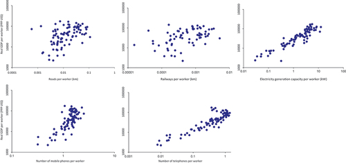
Figure 1 plots the relationship between real GDP per worker and the various infrastructure indicators in the 87-country panel. It indicates that across countries higher infrastructure per worker is associated with higher real GDP per worker. This relationship is particularly strong for electricity generation capacity (r = 0.77) and the telecommunications variables (r = 0.52 and r = 0.67 for mobile and fixed line telephones, respectively).

Figure 1. Real GDP per worker and infrastructure variables, 1992–2017 country means.

IV. Econometric methods

Background

Economic growth is an economy-wide, dynamic process with effects that cannot be fully captured by micro studies, and, therefore, macroeconomic analysis is important. It is likely to be easier to find evidence for causal effects using disaggregated micro-level data rather than using macro-level data (Lee, Miguel, and Wolfram 2020; Asher and Novosad, 2020). This is because some variables may more easily be considered exogenous at the micro-level, and randomized trials and other field experiments are possible. But it does not seem very plausible that we can find exogenous factors that are correlated with infrastructure development across many countries but do not have direct effects on the economy to use as instrumental variables, though natural experiments might be available for specific countries. So, identifying exogenous shocks using time series or panel data methods is probably the only viable approach.

Ideally, we would identify exogenous shocks to infrastructure using a structural panel vector autoregression (Pedroni 2013). There are three main challenges to using such an approach. First, both common and country-specific shocks can be formulated. With a large cross-sectional dimension, a very large number of parameters and impulse response functions will be estimated. If we are interested in the typical effects of infrastructure on development, this information will need to be summarized in some way. The best way to summarize the uncertainty in these summary measures is not clear. Second, the VAR approach requires us to model each of the dependent variables when we are only really interested in the GDP equation. Third, we need to formulate identifying restrictions. Methods to empirically identify a panel SVAR using independent component analysis (see Maxand 2020) have not yet been developed. Therefore, potentially questionable theoretical restrictions must be used. The current study can be seen as a step towards the long-term goal of developing such a model.

Therefore, our estimation follows Calderón, Moral‐Benitom, and Servén (2015) in using a dynamic estimator, which allows us to test for the weak exogeneity of the infrastructure variables. Our contribution is to extend the study beyond 2000 and to investigate the importance of new infrastructure types. Calderón, Moral‐Benitom, and Servén (2015) resorted to using the first principal component of three infrastructure measures and Calderón and Servén (2010) also used the first principal component of infrastructure quality variables. In this paper, we use two such composite infrastructure variables, but we also present the results for the disaggregated variables.

Econometric techniques

Our main analysis uses an aggregate production function as the long-run relationship embedded in an ARDL model. We impose constant returns to scale:

(2) $Y_{\mathit{it}}=A_{\mathit{it}}{K}_{it}^{\beta }{\displaystyle \prod _{\mathit{j}=1}^n{G}_j{\mathit{}}_{\mathit{it}}^{{\gamma }_j}}\left(H_{\mathit{it}}{L}_{\mathit{it}}\right)1-\mathit{\beta }-\mathit{\Sigma }{\gamma }_j,\mathit{\beta }0,{\gamma }_{j}0$(2)

where $Y_{\mathit{it}}$ is real GDP in the $\mathit{i}$^th country at time $\mathit{t}$, $\mathit{A}$ is total factor productivity, $\mathit{K}$ is physical capital, $\mathit{H}$ is human capital per worker, and L is labour. The n $G_j$ are different types of infrastructure capital. As infrastructure is part of the overall capital stock, K, the coefficient vector $\mathit{\gamma }$ will reflect the effect of allocating some of the capital stock to infrastructure rather than other forms of capital such as private structures and equipment. This model implies that though GDP is defined as the income of capital and labour, if capital and labour both increase by the same percentage, but infrastructure remains constant, then, if the ${\gamma }_j$ are greater than zero, GDP increases by less than that percentage. In other words, there are decreasing returns holding infrastructure constant but constant returns when it grows at the same rate as other capital. Taking logs, subtracting the log of aggregate human capital ($H_{\mathit{it}}{L}_{\mathit{it}})$ from both sides, and introducing an error term, $u_{\mathit{it}}$, which is likely to be serially correlated, we have:

(3) $\begin{array}{c}{y}_{\mathit{it}}-h_{\mathit{it}}=a_{\mathit{it}}+\mathit{\beta }\left(k_{\mathit{it}}-h_{\mathit{it}}\right)+\sum _{\mathit{j}=1}^n{\gamma }_j\left(g_{\mathit{j},\mathit{it}}-h_{\mathit{it}}\right)+u_{\mathit{it}}\end{array}$(3)

where $a_{\mathit{it}}$ is $\ln A_{\mathit{it}}$, y is $\ln \left(\mathit{Y}/\mathit{L}\right)$, k is $\ln \left(\mathit{K}/\mathit{L}\right)$, h is lnH and the $g_j$ are $\ln \left(G_j/\mathit{L}\right)$. As described above, we use the first two principal components of the infrastructure variables in our estimation. The resulting model is:

(4) $\begin{array}{cc}\mathit{\hspace{0.17em}}& y_{\mathit{it}}-h_{\mathit{it}}=a_{\mathit{it}}+\mathit{\beta }\left(k_{\mathit{it}}-h_{\mathit{it}}\right)+{\tilde{\gamma }}_1\left({\tilde{g}}_{1,\mathit{it}}-h_{\mathit{it}}\right)\\ \mathit{\hspace{0.17em}}& +{\tilde{\gamma }}_2\left({\tilde{g}}_{2,\mathit{it}}-h_{\mathit{it}}\right)+{\tilde{u}}_{\mathit{it}}\end{array}$(4)

Where ${\tilde{g}}_{1,\mathit{it}}$ and ${\tilde{g}}_{2,\mathit{it}}$ are the first two principal components. Then, the elasticity of GDP with respect to form j of infrastructure is:

(5) $\begin{array}{c}\frac{\mathrm{\partial y}}{\mathrm{\partial }{g}_j}={\tilde{\gamma }}_1{\delta }_{\mathit{j}1}+{\tilde{\gamma }}_2{\delta }_{\mathit{j}2}\end{array}$(5)

where ${\tilde{\gamma }}_1$ and ${\tilde{\gamma }}_2$ are the two regression parameters of the principal components in (4) and ${\delta }_{\mathit{j}1}$ and ${\delta }_{\mathit{j}2}$ are coefficients of the respective infrastructure types in the first and second columns of Table 2.

Our main objective is to examine the long-run relationship between infrastructure and economic growth. Pesaran (2006) pointed out that three specification issues need to be addressed when estimating the long-run parameters of (4). First, the long-run relationship (4) should cointegrate, and all the variables should be at most unit-root in levels and stationary in first differences. Hence, we perform both the IPS (Im, Hashem Pesaran, and Shin 2003) and cross-sectionally augmented panel unit-root (CIPS) tests (Pesaran 2007) to find the order of integration of variables considered in the model. We use the Kao (1999), Pedroni (2004), and Westerlund (2005) cointegration tests. The first two tests are based on modified Dickey-Fuller and modified Phillips-Perron test statistics and the Westerlund test is based on a variance ratio for the residuals. The alternative hypothesis for each test is that the time series in each and every country are cointegrated. To test for the maximum number of cointegrating vectors, we use the Larsson, Lyhagen, and Löthgren (2001) LR-bar test based on the average of the Johansen trace test statistics across the individual countries. Because the time dimension is small, we use the Bartlett correction proposed by Johansen (2002). The test statistic is distributed as a standard normal variable, and it is a one-sided test.

In order to treat the estimated parameters as the causal effect of infrastructure on growth, we need to test for the weak exogeneity of the input variables. We do this using the test proposed by Johansen (1992) as laid out in Calderón, Moral‐Benitom, and Servén (2015). This estimates a VAR in first differences of the input variables, adding first differences of output and the error correction terms from the PMG model. If the error correction terms are jointly insignificant, then the input variables are weakly exogenous.

Second, there is the issue of cross-sectional dependence. If cross-sectional dependence in the residuals is not modelled, this can seriously affect inference and even result in bias in the estimates of the regression coefficients (Söderbom et al. 2014). To deal with cross-sectional dependence, we removed the cross-sectional mean from the data before performing the unit-root tests and use time fixed effects in the regression analysis, but we also employ the Pesaran (2021) CD test to check the cross-sectional independence of the residuals. Third, as countries vary regarding their income level, resources, geographic locations etc., we should take cross-country parameter heterogeneity into consideration when estimating Equation (4)(4) $\begin{array}{cc}\mathit{\hspace{0.17em}}& y_{\mathit{it}}-h_{\mathit{it}}=a_{\mathit{it}}+\mathit{\beta }\left(k_{\mathit{it}}-h_{\mathit{it}}\right)+{\tilde{\gamma }}_1\left({\tilde{g}}_{1,\mathit{it}}-h_{\mathit{it}}\right)\\ \mathit{\hspace{0.17em}}& +{\tilde{\gamma }}_2\left({\tilde{g}}_{2,\mathit{it}}-h_{\mathit{it}}\right)+{\tilde{u}}_{\mathit{it}}\end{array}$(4) (Pesaran, Shin, and Smith 1999).

We use the Pesaran, Shin, and Smith (1999) Pooled Mean Group (PMG) estimator that is embedded in an autoregressive distributed lag (ARDL) framework and models heterogenous short-run dynamics:

(6) $\begin{array}{rl}& \mathrm{\Delta }{\hat{y}}_{\mathit{it}}={\varphi }_i\left({\hat{y}}_{\mathit{it}-1}-{{\mathbf{x}}_{\mathit{it}-1}}^{\mathrm{\prime }}\mathit{\theta }\right)+\sum _{\mathit{j}=1}^{\mathit{p}-1}{\psi }_{\mathit{ij}}\mathrm{\Delta }{\hat{y}}_{\mathit{it}-\mathit{j}}\\ & +\sum _{\mathit{k}=0}^{\mathit{q}-1}\mathbf{\Delta }{{\mathbf{x}}_{\mathit{it}-\mathit{k}}}^{\mathrm{\prime }}{\mathit{\zeta }}_{\mathit{ik}}+{\mu }_i+{\lambda }_t+{\epsilon }_{\mathit{it}}\end{array}$(6)

Where ${\hat{y}}_{\mathit{it}}=y_{\mathit{it}}-h_{\mathit{it}}$, $\mathbf{x}{ }^{\mathrm{\prime }}=\left[k_{\mathit{it}}-h_{\mathit{it}},{\tilde{g}}_{1,\mathit{it}}-h_{\mathit{it}},{\tilde{g}}_{2,\mathit{it}}-h_{\mathit{it}}\right]$, ${\mu }_i$ is a country fixed effect, ${\lambda }_t$ is a time effect common across countries, and ${\epsilon }_{\mathit{it}}$ is an independent and identically distributed random error term. The first term on the RHS models adjustment towards the long-run equilibrium, while the second and third terms model short-run dynamics. We used the replication file provided by RATS for Pesaran, Shin, and Smith (1999) to develop our code using static fixed effects as the initial long-run coefficient vector. We also estimate the model separately for developing and developed countries. Finally, to examine the robustness of our results to data sources, we estimate the model using the World Bank PPP GDP series.

V. Results and discussion

Panel unit root and cointegration tests

Table 4 presents the result of the IPS and Pesaran (2007) CIPS tests. The number of mobile phones is trend stationary according to both the IPS and Pesaran CIPS test. Both tests suggest that all other individual variables contain a unit root and become stationary after differencing. Therefore, we find that all variables except mobile phones are integrated of order one. According to the IPS test the second principal component is trend stationary. But the CIPS test finds that it is only stationary in levels.

Table 4. Panel unit root tests.

Variable	IPS (2003)		Pesaran CIPS (2007)
	Level	First difference	Level	First difference
GDP	2.928	−7.035***	−2.479	−4.334***
Physical capital	2.130	−5.008***	−2.575	−3.357***
Human capital	2.541	−4.394***	−1.622	−3.531***
Electricity generation	−0.390	−7.320***	−2.358	−4.375***
Roads	0.238	−7.322***	−2.051	−4.029***
Railways	0.371	−6.136***	−1.482	−3.126***
Mobile phones	−7.835***	−16.863***	−3.973***	−4.690***
Telephones	4.359	−3.055***	−1.797	−3.870***
1^st PC	−1.457	−7.734***	−2.378	−4.214***
2^nd PC	−2.925***	−9.609***	−2.365	−3.915***

All variables are expressed in logs (or IHS) and per worker. For the IPS (2003) and Pesaran (2007) CIPS test we include a trend and two lags. The null hypothesis of both tests is the existence of unit roots. *** significant at 1%.

Table 5 presents the results of the Kao, Pedroni, and Westerlund panel cointegration tests. As mentioned above, the alternative hypothesis in each case is that the time series cointegrate in every country. All three test statistics reject the null hypothesis of no cointegration. Table 6 presents the results of the Larsson, Lyhagen, and Löthgren (2001) LR-bar test. The critical value for the LR-bar statistic at the 5% level is 1.65. As we can reject zero cointegrating vectors, but not the hypothesis of one cointegrating vector, the maximum cointegrating rank is one.

Table 5. Panel cointegration tests.

Test	Test statistic
Kao (1999) Modified Dickey -Fuller	2.929***
Pedroni (2004) Modified Phillips-Perron	3.737***
Westerlund (2005) Variance ratio	3.251***

*** indicates the 1% and ** the 5% significance levels. Kao and Pedroni tests use two lags and the Westerlund test includes a trend and cross-sectionally demeans the data.

Table 6. LR-bar test of maximum cointegration rank.

Rank	LR-bar statistic
0	6.11
1	−3.32
2	1.54
3	0.07

The LR-bar test is one sided with a critical value of 1.65 at the 5% level.

Coefficient estimates

We consider maximum values for p and q in (6) of three (two lags of the first differences). We use the Akaike Information Criterion based on the likelihood function in Pesaran, Shin, and Smith (1999) to select the optimal lag length. We do not choose different lag lengths for each country. Effectively, we are choosing a maximum lag length for all countries. Excess lag coefficients can be estimated as zero. Table 7 shows that the optimal lag length is two lags of both the dependent variable and the independent variables (one lagged first difference). The parameter estimates are quite similar for all models with $\mathit{q}\ge 2$. The infrastructure elasticities are smaller for models with $\mathit{q}=1$.

Table 7. Lag length selection using akaike information criterion.

	p=1	p=2	p=3
q=1	−9577	−9508	−9391
q=2	−9593	−9600	−9564
q=3	−9406	−9424	−9500

The first column of Table 8 reports pooled mean group (PMG) estimates of the long-run parameters and the rate of adjustment coefficient. Coefficients for subsamples and the World Bank data are discussed below. The output elasticities of the physical and human capital variables seem reasonable. The coefficients of the infrastructure variables are positive and highly significant. The elasticities are very large compared to previous estimates such as Calderón, Moral‐Benitom, and Servén (2015). The relatively low value of the adjustment coefficient shows that GDP responds slowly to changes in infrastructure as we would expect.

Table 8. Pooled mean group estimates – long-run parameters.

	Full Sample, PWT Data	Developing Countries, PWT Data	Developed Countries, PWT Data	Full Sample, World Bank Data
Physical capital	0.299***	0.384***	0.284***	0.313***
	(0.018)	(0.014)	(0.037)	(0.018)
1^st PC	0.180***	0.228***	0.160***	0.199***
	(0.011)	(0.010)	(0.017)	(0.011)
2^nd PC	0.119***	0.009	0.069***	0.104***
	(0.013)	(0.015)	(0.020)	(0.012)
Human capital	0.401***	0.379***	0.487***	0.383***
	(0.019)	(0.020)	(0.030)	(0.021)
Adjustment coefficient	−0.125***	−0.092***	−0.109***	−0.126***
	(0.018)	(0.014)	(0.037)	(0.018)
CD test p-value	0.657	0.299	0.049	0.121
Weak exogeneity p-value	0.090	0.202	0.202	0.020
p	2	1	3	2
q	2	2	1	2
Observations	2,088	1152	897	2088

The table reports the long-run elasticities $\mathit{\theta }$ for each of the inputs and the adjustment coefficient $\mathit{\varphi }$. The adjustment coefficient is the mean across all countries. The CD test null hypothesis is cross-section independence. Standard errors are in parentheses. ***, **, and * significant at the 1%, 5%, and 10% levels respectively.

The first principal component, which we interpret as mainly an electricity and telecommunications factor has double the effect on GDP than the second principal component, which we interpret as mainly a transport factor, does. Together they have about the same effect on GDP as physical capital in general. As described in (5), we can also compute long-run elasticities of GDP with respect to the individual types of infrastructure (Table 9). Roads, railways, and telephones have similar large elasticities and mobile phones and railways small elasticities.

Table 9. Elasticities of infrastructure variables.

	Full Sample	Developing	Developed
Roads	0.099	0.031	0.079
Railways	0.003	−0.027	−0.007
Electricity	0.100	0.125	0.078
Mobile phones	0.008	0.011	0.007
Telephones	0.090	0.097	0.072

Among the telecommunications infrastructure types, we estimate a larger elasticity for fixed line phones than for mobile phones. However, mobile phones have grown in number much more rapidly and so the small elasticity does not reflect a necessarily small contribution to growth. While the mean number of fixed telephone lines per worker was unchanged from 1992 to 2017, the mean number of mobile phones increased by a factor of 144 or in natural logarithms almost 5 (Table 3). Microeconomic research has identified positive impacts of income from mobile and smart phones (Hübler and Hartje 2016). Although we have assumed that elasticities are constant, in reality they likely depend on the level of the inputs.

Table 8 includes the Pesaran (2021) CD test. This shows that the residuals are cross-sectionally independent. We also carry out the test for weak exogeneity, which has a p-value of 0.09. Hence, we cannot reject the null hypothesis of weak exogeneity, and we can interpret the PMG elasticities as causal effects.

As a robustness test, we also estimate the PMG model using GDP in 2017 PPP dollars from the World Bank Development Indicators (Table 8). In the latter dataset some countries have missing data in the first few years. We used the growth rates of RGDPO from PWT 10 to fill in these missing observations. We impose the same lag length as in our main estimate. The coefficient estimates are very similar to our main estimate. However, we can reject the weak exogeneity hypothesis for this sample at the 5% level.

Development status

Table 8 also reports results for the PMG estimator separately for developing and developed countries. Tables 10a and 10b report the AIC for alternative lag lengths for these sub-samples. As a result, we chose p = 1, q = 2 for the developing country sample and p = 3, q = 1 for the developed country sample. The coefficient of the second principal component is not statistically significant for the developing country sample. The coefficients of both principal components are smaller in the developed country sample than in the full sample, though both are statistically significant. The Pesaran CD test narrowly rejects the null of no cross-sectional correlation of the residuals in the developed country sample.5

Table 10. a. Lag length selection using akaike information criterion – developing countries. b. Lag length selection using Akaike information criterion – developed countries.

	p=1	p=2	p=3
a
q=1	−4819	−4835	−4743
q=2	−4936	−4913	−4813
q=3	−4831	−4753	−4706
b
q=1	−4403	−4425	−4719
q=2	−4388	−4353	−4679
q=3	−4679	−4672	−4691

Again, we cannot reject the null of the weak exogeneity of the regressors. The p-values for both sub-samples are coincidentally very close.

Table 9 also presents estimates of the elasticities of GDP with respect to the individual forms of infrastructure in the two development sub-samples. Based on this, the elasticities for transport infrastructure are much smaller in the developing country sample and those for electricity and communication area a little larger than in the full sample. In the developed economies all the elasticities are somewhat smaller than in the full sample.

Long-run versus short-run effects

As we have estimated a dynamic panel model, we can compute both short-run and long-run elasticities. We recover the average short-run parameters across the sample by estimating a mean-group model imposing the cointegrating vector estimated by PMG. Figure 2 reports the impulse response curves of GDP to changes in the two principal components for the full sample estimates:

Figure 2. Response of GDP to increase in infrastructure.

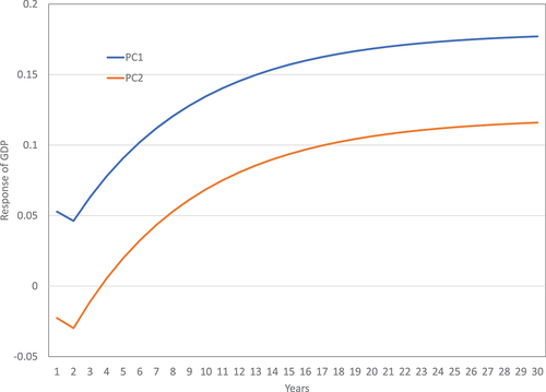
Figure 2 shows that in the full sample, not only does transport infrastructure, which is mainly associated with the second principal component, have a smaller long-run effect than electricity and telecommunications, in the short run its effect is negative. Similarly, Ramey (2018) found a negative short-run effect for road infrastructure in the United States. However, even for electricity and telecommunications, which are mainly associated with the first principal component, the short-run effect is only about a quarter of the final long-run effect. This suggests that studies that find small effects of infrastructure provision (e.g. Lee, Miguel, and Wolfram 2020) need to adopt a much longer-run time frame for program evaluation.⁶

VI. Conclusions and policy implications

We extended previous research on the role of infrastructure in economic growth to recent decades (1992–2017) and to also include new types of infrastructure, such as mobile telephones. Our study shows three major insights. First, we find larger long-run effects of infrastructure on growth than the previous best studies found. Specifically, our main results find long-run elasticities of GDP of 0.09 to 0.1 with respect to each of roads, electricity generation capacity, and telephones. Second, we find that electricity and communications infrastructure have somewhat greater impact in developing economies than in developed economies but transport infrastructure has much less effect in developing economies. Third, the short-run effects of infrastructure are small and in the case of transport infrastructure may be negative.

These findings can be explained through the use of recent data sets covering developing countries where lack of infrastructure is a major development bottleneck. These findings suggest that inputs that are limiting factors or ‘binding constraints’ (McCulloch and Zileviciute, 2017; Burke, Stern, and Bruns 2018) are likely to make more difference to output if their quantity increases. In the short run, infrastructure investment can be disruptive (Ramey 2018) and other complementary investments are needed to fully exploit the potential of new infrastructure.

The findings of this study imply important policy considerations. The higher impacts of telecommunications and electricity indicate that economic growth can be stimulated through better information that enhances market access to products, potential productivity gains through increased substitution possibilities facilitated by information services, or through better telecommunication access. Providing telecommunication services is cheaper than providing transportation and electricity services although there would be very little substitution between them. Another policy implication is that infrastructure whose unavailability has already created barriers to economic development has to be addressed first. In other words, an optimal investment in infrastructure is critical. Instead of providing ‘too much’ road infrastructure like in the United States, an optimal road infrastructure where use of roads (services obtained from road infrastructure) instead of availability of roads (i.e. just increasing stock of road infrastructures) can be maximized.

We collected data on a wide range of other infrastructure variables, such as the number of airports or the percentage of roads that are paved, but these were very limited in time dimension or the number of countries for which data were available. Future research on the effects of infrastructure on growth would benefit from extending collection or estimation of these variables, particularly in the time dimension.

Acknowledgement

We wouldlike to thank Gal Hochman, Pravakar Sahoo, Fan Zhang, and ananonymous referee for their valuable comments and suggestions.

Disclosure statement

Govinda Timilsina is employed by the World Bank. This work was supported by a World Bank Research Support Grant (RSB), which funded Debasish Das. The views and interpretations are of the authors and should not be attributed to the World Bank Group and the organizations they are affiliated with. David Stern has no declarations to make..

Additional information

Funding

The work was supported by the World Bank.

Notes

¹ Elburz, Nijkamp, and Pels (2017) conducted a meta-analysis of 42 empirical studies published between 1995 and 2014 highlighting the sensitivity of results to various factors.

² See Ramey (2020) for a recent review of evidence for the United States.

³ We use the most recent classification: https://datahelpdesk.worldbank.org/knowledgebase/articles/906519-world-bank-country-and-lending-groups.

⁴ The highest correlation between pairs of these demeaned variables is 0.52 between mobile and ifxed line telephones.

⁵ Following the suggestion of a referee, we also estimated the Pesaran (2006) CCEMG estimator for this sample. Because of all the additional regressors, there are only three degrees of freedom in each individual country regression. The results are in Table B1.

⁶ We also estimated cross-section growth models of the following form.

$\begin{array}{c}{y}_{\mathit{it}}-y_{\mathit{it}-5}={\alpha }_0+{\mathit{\delta }}^{\prime }{\mathit{z}}_{\mathit{it}-5}+e_{\mathit{it}}\end{array}$

where ${\mathit{z}}_{\mathit{it}-5}$ is a vector of the initial values of a set of variables including infrastructure variables and initial GDP per-capita. The latter variable controls for many unobserved determinants of growth. These regressions allow us to use a wider range of infrastructure variables that are not available as extensive time series, such as airports. On the whole, the coefficients of the infrastructure variables were statistically insignificant in these regressions, and we do not report them in this paper. This implies that higher levels of infrastructure are not associated with more rapid economic growth.

Appendices

Appendix A

We extracted real GDP, capital stock, human capital, and employment data from Penn World Table 10 (Feenstra, Inklaar, and Timmer 2015). We use the “rgdpna” series which measures real GDP in constant 2017 US PPP dollars, using the growth rates from countries’ national accounts. We use the “rnna” capital stock series, which is also in constant 2017 US PPP dollars, using the growth rates from countries’ national accounts. We refer to this in the following as “physical capital” to distinguish it from human capital. To test the robustness of our analysis to data sources we also used World Bank data on PPP adjusted GDP (World Development Indicators). The human capital stock is measured by the “hc” series which is an index based on years of schooling and returns to education Inklaar and Timmer (2013). Lastly, we use the “emp” series which captures number of persons engaged in work force to measure labour input. We divide GDP and capital stock by labour and take natural logarithms of these variables.

For infrastructure, we assembled data for both quantity and quality of infrastructure variables. We prepared data in three broad categories: Transport, Telecommunications, and Energy as follows.

Transport

Road quantity: We use two editions of World Road Statistics from the International Road Federations for the periods 1990-2007 and 2000-2017 to prepare the length of road network (in kilometres). We also received data from Cesar Caldéron that is derived from similar sources. We merged the datasets as follows:

1. Where the values for 2000 in the two WRS datasets matched we just merged the two series.

2. Where they did not, but the Calderon data did match the 2000-2017 WRS data we used the Calderon data for years before 2000.

3. Where neither matched exactly we used the implied growth rates in either earlier data set to project back from 2000 to 1990.

4. We linearly interpolated missing values.

5. Additionally, we deleted the data point for UAE in 2000 for being anomalously low. We removed the first 1 from the numbers for Botswana for 1992-4. We deleted the datapoint for Bulgaria 2005.

6. Finally, 11 countries had missing data for 2017, in that case we extrapolated the missing 2017 data by keeping same value as stated in 2016. If there was no or little growth in the road network prior to 2016. There were six countries where that was possible: Belgium, Lao PDR, New Caledonia, Papua New Guinea, Thailand and Vietnam.

Railways: The length of railways in km is obtained from the World Bank’s Development Indicators Database, Knoema (2020) database and complemented by data from national sources referenced in Wikipedia. For some countries, we drop apparently bad data and replaced it with data from official government statistics. For instance, for Australia we obtained data from the Bureau of Infrastructure and Transport Research (2020). We also linearly interpolated some missing or obviously incorrect datapoints.

Telecommunications

Telecommunications: Number of mobile phones subscribers and number of telephone lines data are taken from the International Telecommunication Union’s (2020) World Telecommunication/ICT Indicators database.

Energy

Electricity generation capacity data (in megawatts) extracted from the UN Energy Statistics Database (2020).

All variables are converted to per worker values with the exception of human capital which is already in per worker form. All variables apart from mobile phones, and railways are converted to natural logarithms. As there are many 0 values for the number of mobile phones and the length of railways, we use the inverse hyperbolic sine (IHS) transformation for these variables given by $\mathit{ln}\left(\mathit{x}+\sqrt{x^2+1}\right)$ instead of logarithms.

Table A1. List of countries.

Argentina	Costa Rica	Indonesia	Moldova	Portugal
Armenia	Cyprus	Iran	Mongolia	Qatar
Australia	Denmark	Ireland	Morocco	Russian Federation
Austria	Dominican Republic	Israel	Mozambique	Saudi Arabia
Bahrain	Ecuador	Jamaica	Myanmar	Senegal
Bangladesh	Egypt	Japan	Namibia	Singapore
Belgium	Estonia	Jordan	Nepal	Slovenia
Bolivia	Finland	Kazakhstan	Netherlands	Spain
Botswana	France	Kenya	New Zealand	Switzerland
Brazil	Gambia	Korea, Rep.	Nicaragua	Tanzania
Brunei Darussalam	Germany	Kuwait	Niger	Tunisia
Bulgaria	Greece	Latvia	Norway	Turkey
Burkina Faso	Guatemala	Lithuania	Pakistan	Ukraine
Cameroon	Honduras	Luxembourg	Panama	United Kingdom
Canada	Hong Kong	Malaysia	Paraguay	United States
Chile	Hungary	Mali	Peru
China	Iceland	Mauritius	Philippines
Colombia	India	Mexico	Poland

High income countries (World Bank) are written in italics.

Appendix B

Table B1. CCEMG – long-run parameters.

	Developed Countries, PWT Data
Physical capital	0.487***
	(0.091)
1^st PC	0.238***
	(0.044)
2^nd PC	−0.586***
	(0.089)
Human capital	0.861***
	(0.068)
Adjustment coefficient	−0.706***
	(0.078)
p	3
q	1
Observations	897

The table reports the long-run elasticities $\mathit{\theta }$ for each of the inputs and the adjustment coefficient $\mathit{\varphi }$. Standard errors are in parentheses. ***, ** and * significant at the 1%, 5% and 10% level respectively.

References

- Ajakaiye, O., and M. Ncube. 2010. “Infrastructure and Economic Development in Africa: An Overview.” Journal of African Economies 19 (suppl_1): i3–12. doi:10.1093/jae/ejq003.
- Arellano, M., and S. Bond. 1991. “Some Tests of Specification for Panel Data: Monte Carlo Evidence and an Application to Employment Equations.” The Review of Economic Studies 58 (2): 277–297. doi:10.2307/2297968.
- Arellano, M., and O. Bover. 1995. “Another Look at the Instrumental Variable Estimation of Error-Components Models.” Journal of Econometrics 68 (1): 29–51. doi:10.1016/0304-4076(94)01642-D.
- Aschauer, D. A. 1989. “Is Public Expenditure Productive?” Journal of Monetary Economics 23 (2): 177–200. doi:10.1016/0304-3932(89)90047-0.
- Asher, S., and P. Novosad. 2020. “Rural Roads and Local Economic Development.” The American Economic Review 110 (3): 797–823. doi:10.1257/aer.20180268.
- Bazzi, S., and M. A. Clemens. 2013. “Blunt Instruments: Avoiding Common Pitfalls in Identifying the Causes of Economic Growth.” American Economic Journal: Macroeconomics 5 (2): 152–186. doi:10.1257/mac.5.2.152.
- Bun, M. J. G., and F. Windmeijer. 2010. “The Weak Instrument Problem of the System GMM Estimator in Dynamic Panel Data Models.” The Econometrics Journal 13 (1): 95–126. doi:10.1111/j.1368-423X.2009.00299.x.
- Burke, P. J., D. I. Stern, and S. B. Bruns. 2018. “The Impact of Electricity on Economic Development: A Macroeconomic Perspective.” International Review of Environmental and Resource Economics 12 (1): 85–127. doi:10.1561/101.00000101.
- Calderón, C., E. Moral‐benitom, and L. Servén. 2015. “Is Infrastructure Capital Productive? A Dynamic Heterogeneous Approach.” Journal of Applied Econometrics 30 (2): 177–198. doi:10.1002/jae.2373.
- Calderón, C., and L. Servén. 2010. “Infrastructure and Economic Development in Sub-Saharan Africa.” Journal of African Economies 19 (suppl_1): i13–87. doi:10.1093/jae/ejp022.
- Chakamera, C., and P. Alagidede. 2018. “The Nexus Between Infrastructure (Quantity and Quality) and Economic Growth in Sub Saharan Africa.” International Review of Applied Economics 32 (5): 641–672. doi:10.1080/02692171.2017.1355356.
- Cook, P. 2011. “Infrastructure, Rural Electrification and Development.” Energy for Sustainable Development 15 (3): 304–313. doi:10.1016/j.esd.2011.07.008.
- Cook, L. M., and Munnell, A. H. September, 1990. “How Does Public Infrastructure Affect Regional Economic Performance?” New England Economic Review (September): 11–33.
- Dash, R. K., and P. Sahoo. 2010. “Economic Growth in India: The Role of Physical and Social Infrastructure.” Journal of Economic Policy Reform 13 (4): 373–385. doi:10.1080/17487870.2010.523980.
- Démurger, S. 2001. “Infrastructure Development and Economic Growth: An Explanation for Regional Disparities in China?” Journal of Comparative Economics 29 (1): 95–117. doi:10.1006/jcec.2000.1693.
- Donaldson, D. 2018. “Railroads of the Raj: Estimating the Impact of Transportation Infrastructure.” The American Economic Review 108 (4–5): 899–934. doi:10.1257/aer.20101199.
- Donaldson, D., and R. Hornbeck. 2016. “Railroads and American Economic Growth: A “Market Access” Approach.” The Quarterly Journal of Economics 131 (2): 799–858. doi:10.1093/qje/qjw002.
- Duffy-Deno, K. T., and R. W. Eberts. 1991. “Public Infrastructure and Regional Economic Development: A Simultaneous Equations Approach.” Journal of Urban Economics 30 (3): 329–343. doi:10.1016/0094-1190(91)90053-A.
- Elburz, Z., P. Nijkamp, and E. Pels. 2017. “Public Infrastructure and Regional Growth: Lessons from Meta-Analysis.” Journal of Transport Geography 58: 1–8. doi:10.1016/j.jtrangeo.2016.10.013.
- Estache, A., B. Speciale, and D. Veredas. 2005. “How Much Does Infrastructure Matter to Growth in Sub-Saharan Africa.” unpublished WorldBank (June 2005).
- Faber, B. 2014. “Trade Integration, Market Size, and Industrialization: Evidence from China’s National Trunk Highway System.” The Review of Economic Studies 81 (3): 1046–1070. doi:10.1093/restud/rdu010.
- Fan, S., and X. Zhang. 2004. “Infrastructure and Regional Economic Development in Rural China.” China Economic Review 15 (2): 203–214. doi:10.1016/j.chieco.2004.03.001.
- Feenstra, R. C., R. Inklaar, and M. P. Timmer. 2015. “The Next Generation of the Penn World Table.” The American Economic Review 105 (10): 3150–3182. doi:10.1257/aer.20130954.
- Garcia-Mila, T., and T. J. McGuire. 1992. “The Contribution of Publicly Provided Inputs to States’ Economies.” Regional Science and Urban Economics 22 (2): 229–241. doi:10.1016/0166-0462(92)90013-Q.
- German-Soto, V., and H. A. Barajas Bustillos. 2014. “The Nexus Between Infrastructure Investment and Economic Growth in the Mexican Urban Areas.” Modern Economy 5 (13): 1208–1220. doi:10.4236/me.2014.513112.
- Hübler, M., and R. Hartje. 2016. “Are Smartphones Smart for Economic Development?” Economics Letters 141: 130–133. doi:10.1016/j.econlet.2016.02.001.
- Im, K. S., M. Hashem Pesaran, and Y. Shin. 2003. “Testing for Unit Roots in Heterogeneous Panels.” Journal of Econometrics 115 (1): 53–74. doi:10.1016/S0304-4076(03)00092-7.
- Inklaar, R., and M. P. Timmer. 2013. “Capital, Labor, and TFP in PWT8.0.” Groningen Growth and Development Centre, University of Groningen.
- Johansen, S. 1992. “Cointegration in Partial Systems and the Efficiency of Single-Equation Analysis.” Journal of Econometrics 52 (3): 389–402. doi:10.1016/0304-4076(92)90019-N.
- Johansen, S. 2002. “A Small Sample Correction for the Test of Cointegrating Rank in the Vector Autoregressive Model.” Econometrica 70 (5): 1929–1961. doi:10.1111/1468-0262.00358.
- Kao, C. 1999. “Spurious Regression and Residual-Based Tests for Cointegration in Panel Data.” Journal of Econometrics 90 (1): 1–44. doi:10.1016/S0304-4076(98)00023-2.
- Knoema. 2020. World and national data, maps & rankings. https://knoema.com/atlas
- Kodongo, O., and K. Ojah. 2016. “Does Infrastructure Really Explain Economic Growth in Sub-Saharan Africa?” Review of Development Finance 6 (2): 105–125. doi:10.1016/j.rdf.2016.12.001.
- Lall, C. M. 1999. “India Spruces Up Its IP Regime and Its Enforcement.” The Journal of World Intellectual Property 2 (6): 961–968. doi:10.1111/j.1747-1796.1999.tb00101.x.
- Larsson, R., and J. Lyhagen. 2000. “Testing for Common Cointegrating Rank in Dynamic Panels.” Working Paper Series in Economics and Finance, 378. Stockholm School of Economics.
- Larsson, R., J. Lyhagen, and M. Löthgren. 2001. “Likelihood‐based Cointegration Tests in Heterogeneous Panels.” The Econometrics Journal 4 (1): 109–142. doi:10.1111/1368-423X.00059.
- Lee, K., E. Miguel, and C. Wolfram. 2020. “Does Household Electrification Supercharge Economic Development?” Journal of Economic Perspectives 34 (1): 122–144. doi:10.1257/jep.34.1.122.
- Lewis, B. D. 1998. “The Impact of Public Infrastructure on Municipal Economic Development: Empirical Results from Kenya.” Review of Urban & Regional Development Studies 10 (2): 142–156. doi:10.1111/j.1467-940X.1998.tb00092.x.
- Maxand, S. 2020. “Identification of Independent Structural Shocks in the Presence of Multiple Gaussian Components.” Econometrics and Statistics 16: 55–68. doi:10.1016/j.ecosta.2018.10.005.
- McCulloch, N., and D. Zileviciute. 2017. “Is Electricity Supply a Binding Constraint to Economic Growth in Developing Countries?” EEG State-of-Knowledge Paper 1.3.
- Mohd, J. M., W. I. Normaz, and S. H. Law. 2012. “A Pooled Mean Group Estimation on ICT Infrastructure and Economic Growth in ASEAN-5 Countries.” International Journal of Economics and Management 6 (2): 360–378.
- Morrison, C. J., and A. E. Schwartz. 1996. “State Infrastructure and Productive Performance.” The American Economic Review 86 (5): 1095–1111.
- Morten, M., and J. Oliveira. 2018. “The Effects of Roads on Trade and Migration: Evidence from a Planned Capital City.” NBER Working Papers, 22158.
- Mostert, J. W., and J. H. Van Heerden. 2015. “A Computable General Equilibrium (CGE) Analysis of the Expenditure on Infrastructure in the Limpopo Economy in South Africa.” International Advances in Economic Research 21 (2): 227–236. doi:10.1007/s11294-015-9524-1.
- Nketiah-Amponsah, E. 2009. “Public Spending and Economic Growth: Evidence from Ghana (1970–2004).” Development Southern Africa 26 (3): 477–497. doi:10.1080/03768350903086846.
- Pedroni, P. 2004. “Panel Cointegration: Asymptotic and Finite Sample Properties of Pooled Time Series Tests with an Application to the PPP Hypothesis.” Econometric Theory 20 (03): 597–625. doi:10.1017/S0266466604203073.
- Pedroni, P. 2013. “Structural Panel Vars.” Econometrics 1 (2): 180–206. doi:10.3390/econometrics1020180.
- Pesaran, M. H. 2006. “Estimation and Inference in Large Heterogeneous Panels with a Multifactor Error Structure.” Econometrica 74 (4): 967–1012. doi:10.1111/j.1468-0262.2006.00692.x.
- Pesaran, M. H. 2007. “A Simple Panel Unit Root Test in the Presence of Cross‐section Dependence.” Journal of Applied Econometrics 22 (2): 265–312. doi:10.1002/jae.951.
- Pesaran, M. H. 2021. “General Diagnostic Tests for Cross-Sectional Dependence in Panels.” Empirical Economics 60: 13–50. doi:10.1007/s00181-020-01875-7.
- Pesaran, M. H., Y. Shin, and R. P. Smith. 1999. “Pooled Mean Group Estimation of Dynamic Heterogeneous Panels.” Journal of the American Statistical Association 94 (446): 621–634. doi:10.1080/01621459.1999.10474156.
- Ramey, V. A. 2018. “Fiscal Policy: Tax and Spending Multipliers in the U.S.” In Evolution or Revolution: Rethinking Macroeconomic Policy After the Great Recession, edited by O. Blanchard and L. H. Summers, 71–162. Cambridge, MA: MIT Press.
- Ramey, V. A. 2020. “The Macroeconomic Consequences of Infrastructure Investment.” NBER Working Papers, 14366.
- Rives, J. M., and M. T. Heaney. 1995. “Infrastructure and Local Economic Development.” Journal of Regional Analysis and Policy 25 (1): 58–73.
- Roy, B. C., S. Sarkar, N. R. Mandal, and S. Pandey. 2014. “Impact of Infrastructure Availability on Level of Industrial Development in Jharkhand, India: A District Level Analysis.” International Journal of Technological Learning, Innovation and Development 7 (2): 93–123. doi:10.1504/IJTLID.2014.065880.
- Sahoo, P., and R. K. Dash. 2009. “Infrastructure Development and Economic Growth in India.” Journal of the Asia Pacific Economy 14 (4): 351–365. doi:10.1080/13547860903169340.
- Sahoo, P., and R. K. Dash. 2012. “Economic Growth in South Asia: Role of Infrastructure.” The Journal of International Trade & Economic Development 21 (2): 217–252. doi:10.1080/09638191003596994.
- Sanchez‐Robles, B. 1998. “Infrastructure Investment and Growth: Some Empirical Evidence.” Contemporary Economic Policy 16 (1): 98–108. doi:10.1111/j.1465-7287.1998.tb00504.x.
- Shi, Y., S. Guo, and P. Sun. 2017. “The Role of Infrastructure in China’s Regional Economic Growth.” Journal of Asian Economics 49: 26–41. doi:10.1016/j.asieco.2017.02.004.
- Söderbom, M., F. Teal, M. Eberhardt, S. Quinn, and A. Zeitlin. 2014. Empirical Development Economics. Oxford, New York: Routledge.
- Srinivasu, B., and P. Srinivasa Rao. 2013. “Infrastructure Development and Economic Growth: Prospects and Perspective.” Journal of Business Management & Social Sciences Research 2 (1): 81–91.
- Storeygard, A. 2016. “Farther on Down the Road: Transport Costs, Trade and Urban Growth in Sub-Saharan Africa.” The Review of Economic Studies 83 (3): 1263–1295. doi:10.1093/restud/rdw020.
- Timilsina, G. R., G. Hochman, and Z. Song. 2020. “Infrastructure, Economic Growth, and Poverty: A Review.” World Bank Policy Research Working Paper, no. 9258.
- Urrunaga, R., and C. Aparicio. 2012. “Infrastructure and Economic Growth in Peru.” CEPAL Review 107: 145–163. doi:10.18356/8537fd57-en.
- Westerlund, J. 2005. “New Simple Tests for Panel Cointegration.” Econometric Reviews 24 (3): 297–316. doi:10.1080/07474930500243019.
- World Bank. 2018. “Access to Electricity in Sub-Saharan Africa.” Africa Pulse Report, 17. World Bank: Washington, DC.
- Wylie, P. J. 1996. “Infrastructure and Canadian Economic Growth 1946-1991.” Canadian Journal of Economics/Revue Canadienne d’Economique 29: S350–355. doi:10.2307/136015.