Performance of renewable and non-renewable exchange-traded funds during heightened uncertainty

ABSTRACT

This study adopts a composite threshold model that differentiates between the upside and downside betas of the major US-based renewable and non-renewable exchange-traded funds (ETFs) during heightened uncertainty. It is found that downside betas for both renewable and non-renewable energy ETFs are significantly greater than upside betas. However, in a highly uncertain market, renewable energy ETFs tend to enjoy higher upside gains than the fossil-fuel ETFs. The results suggest that renewable energy ETFs have great potential to generate high returns, but the downside risk associated with renewables should be mitigated by government incentivizing the use of renewables in both domestic and foreign markets. Investing in renewable energy is not only good for the environment but also compared to other investment alternatives (including fossil fuels) it provides better risk-adjusted returns. During the last 5 years, some renewable energy ETFs have even outperformed several well-established sectoral ETFs. This paper finds that there is a more favourable business case for investing in renewables than common perception would suggest.

KEYWORDS:

• Renewable
• energy
• fossil fuel
• investment

JEL CLASSIFICATION:

• E62
• G18
• Q38
• Q42

I. Introduction

Investing in ETFs is an effective way to lower financial risk and generate more stable returns through diversification across different asset classes such as stocks, government and non-government bonds, different sectors, and themes. For instance, VTI enables investors to trade the entire US market with approximately 4000 stocks as if it were just one single stock. The popularity of ETFs has been on the rise since 1993. Dragomirescu-Gaina, Galariotis, and Philippas (2021) state that with relatively low fees and high transparency and liquidity ETFs provide diversification benefits and indirect access to international equities, which are illiquid or otherwise inaccessible. In a comprehensive panel study Marti‐Ballester (2020) examines the key factors influencing the behaviour of investors in renewable energy using a large number of conventional mutual funds together with 76 renewable-energy funds and 109 black-energy funds during the period January 2007-December 2017. This study finds that renewable-energy fund investors are less responsive to past financial performance than are other fund investors.

Using green energy ETFs, a number of studies examine the possibility of transitioning to a low-carbon economy (Andersson, Bolton, and Samama 2016; Dragomirescu-Gaina, Galariotis, and Philippas 2021; Miralles-Quirós and Mar Miralles-Quirós 2019). For example, Dragomirescu-Gaina, Galariotis, and Philippas (2021) use 16 green ETFs and a time-varying herding detection model to study how herding interacts with energy equities’ returns, policy uncertainty and volatility proxies. They state that “changes in investors’ behaviour with respect to green asset allocations require a better information set than in the case of crude oil allocations, for which only information on returns is a relevant driver of behaviour” (Dragomirescu-Gaina, Galariotis, and Philippas 2021, 1). Polemis and Spais (2020) examine the economic and behavioural factors impacting on renewable energy investments in Greece using binomial and quantile regression analysis. They suggest that decisionmakers and government authorities should promote a faster penetration of low-carbon technologies to secure more environmentally sustainable economic and social growth. A number of studies have also explored the relationship between energy consumption and economic growth (Nicholas and Payne 2012; Salim, Hassan, and Shafiei 2014) and find a ‘bidirectional causality between energy consumption and economic growth in both the short- and long-run’ (Nicholas and Payne 2012, 733). Given such an important nexus, the important gap in the literature relates to the risk and return trade-off associated with investing in renewable and non-renewables.

The aim of this paper is to investigate how renewable and non-renewable (fossil-fuel) energy ETFs perform when the US stock market becomes highly uncertain. Eight of the chosen ETFs (tickers ICLN, TAN, QCLN, PBW, ERTH, PBD, FAN and SMOG) represent the largest renewable energy ETFs (in terms of asset under management, AUM) and the remaining five ETFs (tickers XLE, VDE, XOP, IYE, and IXC) are classified as fossil-fuel energy ETFs. The entire market is proxied with an ETF known as VTI, which includes all 3870 companies listed in the US. Inter alia, this study finds that the non-asymmetric betas are estimated to be in the same order of magnitude (i.e. 1.28) for both groups of ETFs. Then, a conventional threshold model is specified to highlight the difference between the upside and downside beta coefficients without capturing the moderating impact of market uncertainty. In this model, all downside betas are significantly larger than upside betas, suggesting that both renewable and non-renewable energy ETFs are very risky as they tend to fall more than they rise in response to changes in the market.

Finally, this paper proposes a composite threshold model in which the upside and downside coefficients are allowed to be moderated by variations in the VIX index as a proxy for market uncertainty or fear. In this composite threshold model, when the market is less uncertain (Regime 1), renewable energy ETFs sustain less drawdowns during market selloffs than that of non-renewable energy ETFs. However, when the market becomes highly uncertain (Regime 2), the average upside beta for renewable energy ETFs is found to be larger than that of the non-renewable energy ETFs. The results of this study present a favourable business case for investing in renewable energy ETFs, particularly when market uncertainty is high, because they enjoy higher returns during market rallies and sustain less losses during market selloffs. In addition, during the last 5-year renewable energy ETFs have also outperformed several well-established sectoral ETFs (including those for non-renewable energy) in terms of three risk-adjusted return ratios (i.e. Treynor, Sharpe and Sortino).

II. Literature review

Investors have long been interested in performance measures that can evaluate the choice between investment opportunities with different risk and return profiles. The conventional performance measures such as the Sharpe (1964) and Treynor (1965) ratios are based on Markovitz’s (1959) mean-variance paradigm, that support the notion that the estimated beta or standard deviation of returns are adequate measures for evaluating the performance of a portfolio. The main problem with these measures is that they penalize both upside and downside return movements (Jiang et al. 2019). Rising asset prices can also reduce both the Sharpe and Treynor ratios but investors usually welcome such positive outcomes. In practice, what worries investors is the extent of negative returns. In response to these shortcomings, Bawa and Lindenberg (1977) and Fishburn (1977) proposed alternative measures of downside risk based on lower partial moments. They argue that if risk is perceived as underperformance relative to a benchmark, then the risk-adjusted measures should be utilizing a second order lower partial moment approach. This led to the popularity of semi-variance metrics like the Sortino ratio (Sortino and Forsey 1996; Sortino and van der Meer 1991) and maximum drawdown measures such as the Calmar, Sterling, Burke, Martin, and Pain ratios (Forbes, Kiselev, and Skerratt 2021; Grobys and Huhta-Halkola 2019; Han and Kong 2022; Kuang 2022; Liu, Wang, and Sui 2022; Molyboga and L’Ahelec 2016; Schuhmacher and Eling 2011; Young 1991).

The above complementary measures have jointly been utilized to evaluate the performance of rival portfolios as both risk and return do matter for investors (Kuang 2022). If these measures are between 0–1, 1–2, 2–3 and greater than 3, the relevant portfolio can be described as suboptimal, acceptable, very good and excellent, respectively. The Sharpe and Treynor ratios are useful in evaluating low-volatile portfolios, whereas the Sortino and Calmar ratios are more appropriate for assessing high-risk portfolios by placing an extreme emphasis on the downside risk, particularly when the sample period is not long enough. According to Eling and Schuhmacher (2007), Eling (2008) and Auer and Schuhmacher (2013), the risk-adjusted return rankings obtained from the Sharpe ratio and the Calmar ratio tend to become similar when the investment horizon lengthens.

The present study is different from previous studies in three aspects. First, previous studies only examined the asymmetric upside and downside co-movements between individual stocks and the whole market, whereas the present study captures the moderating impact of market uncertainty on both upside and downside betas. A number of pioneering studies (e.g. Ang, Chen, and Xing 2006; Chiang, Lee, and Wisen 2004; Dennis, Simlai, and Steven Smith 2017) have also highlighted the importance of distinguishing between positive (upside) and negative (downside) return co-movements between an asset and the market as a whole. Some studies estimate conditional downside betas when market returns fall below a certain value (typically zero), or below a target threshold or below an average return (Atilgan, Demirtas, and Gunaydin 2020; Bawa and Lindenberg 1977; Estrada 2002, 2006; Fisher and D’Alessandro 2021; Jiang et al. 2019; Pettengill, Sundaram, and Mathur 1995; Valadkhani 2022).

However, to the best of my knowledge, none of the previous studies have examined how market uncertainty can influence the asymmetry in downside and upside betas of the renewable and fossil fuel energy ETFs. Second, instead of focusing on individual stocks, the present study investigates the price returns of different groupings of stocks aggregated as ETFs, hence reducing the idiosyncrasies present within individual stocks such as mergers and acquisitions. Third, this article provides answers to the following questions: if the entire US stock market (proxied by VTI) falls, how much do different renewable and non-renewable energy ETFs respond to such changes and how does market uncertainty moderate such asymmetric responses? The findings in this study support the view that overall renewable energy ETFs are less susceptible to drawdowns during market selloffs, particularly when market uncertainty exceeds an endogenously determined ‘fear triggering’ point. Unlike fossil fuel energy ETFs, renewable energy ETFs enjoy larger upside betas while having relatively smaller downside betas when uncertainty levels are elevated. Attention is now directed to the empirical methodology for estimating the upside and downside betas.

III. Empirical methodology

It is important to estimate βs to compare the extent of systematic risk and expected return for different types of assets in comparison with the market as a whole. It should be noted at the outset that ‘there are many ways in which beta can be calculated based on factors such as the choice of time interval and market proxy used in the estimation process’ (Lahtinen, Lawrey, and Hunsader 2018, 156). One can use Equation (1)(1) $(r_{\mathit{it}}-r_{\mathit{ft}})={\alpha }_i+{\beta }_i(r_{\mathit{Mt}}-r_{\mathit{ft}})+{\epsilon }_{\mathit{it}}$(1) to estimate the unconditional CAPM (Capital Asset Pricing Model) beta, which utilizes excess return relatives to a risk-free rate:

(1) $(r_{\mathit{it}}-r_{\mathit{ft}})={\alpha }_i+{\beta }_i(r_{\mathit{Mt}}-r_{\mathit{ft}})+{\epsilon }_{\mathit{it}}$(1)

Where:

r_it = daily return on the i^th security (i.e. the i^th ETF) at time t,

r_Mt = daily return on the whole market proxied by ΔLn(M_t) = Ln(M_t)- Ln(M_t−1),

M_t = the total stock market index or the price of an ETF, representing the entire market,

r_ft = the daily risk-free rate of return,

β_i = the estimated unconditional beta for the i^th ETF,

α_i = the constant term, and

ε_it = the stochastic residual series.

In relation to the specification of Equation (1)(1) $(r_{\mathit{it}}-r_{\mathit{ft}})={\alpha }_i+{\beta }_i(r_{\mathit{Mt}}-r_{\mathit{ft}})+{\epsilon }_{\mathit{it}}$(1) , Agrrawal and Waggle (2010, 14) state that:

more commonly, [Equation (1)(1) $(r_{\mathit{it}}-r_{\mathit{ft}})={\alpha }_i+{\beta }_i(r_{\mathit{Mt}}-r_{\mathit{ft}})+{\epsilon }_{\mathit{it}}$(1) ] does not consider excess returns and simply regress the raw security returns against those of the market. Since the periodic risk-free rate [i.e. daily risk free return] is generally fairly close to zero and subtracted from both sides of the equation, this simplification [Equation (2)](2) $r_{\mathit{it}}={\alpha }_i+{\beta }_i{r}_{\mathit{Mt}}+{\epsilon }_{\mathit{it}}$(2) makes little practical difference.

Based on this useful suggestion, Equation (1)(1) $(r_{\mathit{it}}-r_{\mathit{ft}})={\alpha }_i+{\beta }_i(r_{\mathit{Mt}}-r_{\mathit{ft}})+{\epsilon }_{\mathit{it}}$(1) can be rewritten as follows:

(2) $r_{\mathit{it}}={\alpha }_i+{\beta }_i{r}_{\mathit{Mt}}+{\epsilon }_{\mathit{it}}$(2)

Equation (2)(2) $r_{\mathit{it}}={\alpha }_i+{\beta }_i{r}_{\mathit{Mt}}+{\epsilon }_{\mathit{it}}$(2) quantifies the unconditional association between the return of an asset and the return from the entire market. However, previous studies have established that asset prices tend to fall together during market selloffs but rise independently in bull markets (see inter alia Ang and Chen 2002; Bae, Karolyi, and Stulz 2003; Bekaert and Guojun 2000; Christie 1982; French, William Schwert, and Stambaugh 1987; Hong, Jun, and Zhou 2007; Karolyi and Stulz 1996; Longin and Solnik 1995). For a detailed account of why there are such asymmetric co-movements in stock returns see Chung, Hyun, and Hong (2019). Without distinguishing between the upside and downside betas, the estimation of Equation (2)(2) $r_{\mathit{it}}={\alpha }_i+{\beta }_i{r}_{\mathit{Mt}}+{\epsilon }_{\mathit{it}}$(2) may lead to an inaccurate trade-off between risk and return in different market conditions. On this same issue, Sebastien and Panariello (2018) state that downside correlations could be stronger than upside correlations because fear is typically more contagious than optimism. To address the issue of asymmetry, Equation (2)(2) $r_{\mathit{it}}={\alpha }_i+{\beta }_i{r}_{\mathit{Mt}}+{\epsilon }_{\mathit{it}}$(2) is modified as follows:

(3) $r_{\mathit{it}}={\alpha }_i+{\epsilon }_{\mathit{it}}+\left\{\begin{array}{c}{\beta }_i^{-}{r}_{\mathit{Mt}}\mathrm{if}\mathrm{\Delta }{\mathrm{M}}_{\mathrm{t}}<0\\ {\beta }_i^{+}{r}_{\mathit{Mt}}\mathrm{if}\mathrm{\Delta }{\mathrm{M}}_{\mathrm{t}}\ge 0\end{array}\right.$(3)

Where β^– and β⁺ show the downside and upside betas, respectively. When daily-market price falls (proxied by ΔM_t <0), the downside beta coefficient for the i^th ETF is measured by β_i^– but when market price rises, the relevant response is measured by the upside beta or β_i⁺.

However, the estimated parameters in Equation (3)(3) $r_{\mathit{it}}={\alpha }_i+{\epsilon }_{\mathit{it}}+\left\{\begin{array}{c}{\beta }_i^{-}{r}_{\mathit{Mt}}\mathrm{if}\mathrm{\Delta }{\mathrm{M}}_{\mathrm{t}}<0\\ {\beta }_i^{+}{r}_{\mathit{Mt}}\mathrm{if}\mathrm{\Delta }{\mathrm{M}}_{\mathrm{t}}\ge 0\end{array}\right.$(3) can also be subject to significant shifts, depending on how volatile or fearful the market is, hence necessitating the use of a composite or interactive threshold model. To test this possibility, one can use the VIX index as a threshold variable in a breaking regression model. The VIX index was first developed by the Chicago Board Options Exchange (CBOE) as one of the most common barometers of market sentiment based on the implied volatility of S&P 500 index options. The VIX index is a forward-looking indicator because it is calculated using the 30-day expected volatility following the measurement date and derived from real-time, mid-quote prices of call and put options.

Among investors an increase (decrease) in the VIX index is typically interpreted as rising (falling) uncertainty in the market. The VIX index is also referred to as the fear index, representing a quantifiable measure of market risk and investors’ sentiments. According to Dragomirescu-Gaina, Galariotis, and Philippas (2021), the VIX index is also considered as an indicator of financial risk and information frictions. In order to allow the downside and upside betas to be influenced by changes in market sentiments, an iterative grid-search is conducted to determine the optimal values for τ in the following composite threshold regression:

(4) $r_{\mathit{it}}={\epsilon }_{\mathit{it}}+\left\{\begin{array}{c}\left.{\alpha }_1+\left\{\begin{array}{c}{\beta }_{1i}^{-}{r}_{\mathit{Mt}}\mathrm{if}\mathrm{\Delta }{\mathrm{M}}_{\mathrm{t}}<0\\ {\beta }_{1i}^{+}{r}_{\mathit{Mt}}\mathrm{if}\mathrm{\Delta }{\mathrm{M}}_{\mathrm{t}}\ge 0\end{array}\right.\right\}\mathrm{if}\mathrm{\Delta }\mathrm{VI}{\mathrm{X}}_{\mathrm{t}-\mathrm{d}}<\mathit{\tau }\\ {\alpha }_2+\left.\left\{\begin{array}{c}{\beta }_{2i}^{-}{r}_{\mathit{Mt}}\mathrm{if}\mathrm{\Delta }{\mathrm{M}}_{\mathrm{t}}<0\\ {\beta }_{2i}^{+}{r}_{\mathit{Mt}}\mathrm{if}\mathrm{\Delta }{\mathrm{M}}_{\mathrm{t}}\ge 0\end{array}\right.\right\}\mathrm{if}\mathrm{\Delta }\mathrm{VI}{\mathrm{X}}_{\mathrm{t}-\mathrm{d}}\ge \mathit{\tau }\end{array}\right.$(4)

Where ΔVIX_t shows the changes in the market sentiment, d is the length of the delay, and ${\epsilon }_t$ is the well-behaved residual series distributed independently and identically with zero mean and finite non-zero variance σ². Unlike Equation (3)(3) $r_{\mathit{it}}={\alpha }_i+{\epsilon }_{\mathit{it}}+\left\{\begin{array}{c}{\beta }_i^{-}{r}_{\mathit{Mt}}\mathrm{if}\mathrm{\Delta }{\mathrm{M}}_{\mathrm{t}}<0\\ {\beta }_i^{+}{r}_{\mathit{Mt}}\mathrm{if}\mathrm{\Delta }{\mathrm{M}}_{\mathrm{t}}\ge 0\end{array}\right.$(3) , at any point in time the intercept terms and betas can switch from Regime 1 (${\alpha }_1$,${\beta }_{1i}^{-}$,${\beta }_{1i}^{+}$) to Regime 2 (${\alpha }_2$,${\beta }_{2i}^{-}$,${\beta }_{2i}^{+}$), depending on the optimal value taken by the ‘threshold variable’ or ΔVIX_t-d. When the market is less (more) fearful, Regime 1 (Regime 2) can provide more accurate estimates of upside and downside betas. The length of the delay is allowed to vary between 1 and 5 days and its optimum length is determined by the Schwarz information criteria (SIC). Having said that, according to Chan (1993), the prior knowledge of d does not influence the asymptotic properties of the estimators. Equation (4)(4) $r_{\mathit{it}}={\epsilon }_{\mathit{it}}+\left\{\begin{array}{c}\left.{\alpha }_1+\left\{\begin{array}{c}{\beta }_{1i}^{-}{r}_{\mathit{Mt}}\mathrm{if}\mathrm{\Delta }{\mathrm{M}}_{\mathrm{t}}<0\\ {\beta }_{1i}^{+}{r}_{\mathit{Mt}}\mathrm{if}\mathrm{\Delta }{\mathrm{M}}_{\mathrm{t}}\ge 0\end{array}\right.\right\}\mathrm{if}\mathrm{\Delta }\mathrm{VI}{\mathrm{X}}_{\mathrm{t}-\mathrm{d}}<\mathit{\tau }\\ {\alpha }_2+\left.\left\{\begin{array}{c}{\beta }_{2i}^{-}{r}_{\mathit{Mt}}\mathrm{if}\mathrm{\Delta }{\mathrm{M}}_{\mathrm{t}}<0\\ {\beta }_{2i}^{+}{r}_{\mathit{Mt}}\mathrm{if}\mathrm{\Delta }{\mathrm{M}}_{\mathrm{t}}\ge 0\end{array}\right.\right\}\mathrm{if}\mathrm{\Delta }\mathrm{VI}{\mathrm{X}}_{\mathrm{t}-\mathrm{d}}\ge \mathit{\tau }\end{array}\right.$(4) can also be re-written as follows:

(5) $r_{\mathit{it}}=\left({\alpha }_{1\mathit{i}}+{\beta }_{1i}^{-}{r}_{\mathit{Mt}}+{\beta }_{1i}^{+}{r}_{\mathit{Mt}}\right).1(\mathrm{\Delta }\mathrm{VI}{\mathrm{X}}_{\mathrm{t}-\mathrm{d}}<\mathit{\tau })+\left({\alpha }_{2\mathrm{i}}+{\beta }_{2\mathrm{i}}^{-}{\mathrm{r}}_{\mathrm{Mt}}+{\beta }_{2\mathrm{i}}^{+}{\mathrm{r}}_{\mathrm{Mt}}\right).\text{break}1(\mathrm{\Delta }\mathrm{VI}{\mathrm{X}}_{\mathrm{t}-\mathrm{d}}\ge \mathit{\tau })+{\epsilon }_{\mathrm{it}}$(5)

Where τ denotes the optimal variation in the VIX index causing a shift in both downside and upside betas, and 1(·) is an indicator function, which equals one if the condition in the parentheses is met and zero otherwise. It is also possible to write Equation (5)(5) $r_{\mathit{it}}=\left({\alpha }_{1\mathit{i}}+{\beta }_{1i}^{-}{r}_{\mathit{Mt}}+{\beta }_{1i}^{+}{r}_{\mathit{Mt}}\right).1(\mathrm{\Delta }\mathrm{VI}{\mathrm{X}}_{\mathrm{t}-\mathrm{d}}<\mathit{\tau })+\left({\alpha }_{2\mathrm{i}}+{\beta }_{2\mathrm{i}}^{-}{\mathrm{r}}_{\mathrm{Mt}}+{\beta }_{2\mathrm{i}}^{+}{\mathrm{r}}_{\mathrm{Mt}}\right).\text{break}1(\mathrm{\Delta }\mathrm{VI}{\mathrm{X}}_{\mathrm{t}-\mathrm{d}}\ge \mathit{\tau })+{\epsilon }_{\mathrm{it}}$(5) in the following compact form:

(6) $r_{\mathit{it}}=\sum _{\mathit{j}=1}^{\mathit{n}=2}{1}_i(\mathit{\tau },\mathrm{\Delta }\mathrm{VI}{\mathrm{X}}_{\mathrm{t}-\mathrm{d}})\cdot \left({\alpha }_{\mathit{ji}}+{\beta }_{ji}^{-}{r}_{\mathit{Mt}}+{\beta }_{ji}^{+}{r}_{\mathit{Mt}}\right)+{\epsilon }_{\mathit{it}}$(6)

Where n denotes the number of the regimes. In order to determine the optimal threshold parameter (i.e. τ) and the ‘nuisance parameter’ (d), the standard practice is to conduct an iterative grid search within multiple sub-samples using an estimation procedure well-documented in Hansen (2011) and Bai and Perron (2003). The number of regimes can also exceed two but only if they are statistically significant. Since only one shift was statistically significant according to the Wald test, this study estimates only two sets (n = 2) of betas in each regime.

IV. Data

Daily ETF prices (5 days per week) were extracted from https://finance.yahoo.com during the sample period (30 June 2008–19 October 2021), totalling 3472 observations. Table 1 presents the salient characteristics (e.g. the inception date, issuer, number of holdings, the expense ratio and total assets under management) of all major renewable and non-renewable energy ETFs in the US under three sub-headings: eleven recently launched renewable energy ETFs; eight well-established renewable ETFs; and five well-established non-renewable (fossil-fuel) energy ETFs. All ETFs in Table 1 are sorted in descending order based on the value of assets under management. Due to the small number of available observations, the 11 new-renewable energy ETFS have not been included in this study because they were all created after 2015 and their constituents are mainly present in the eight well-established renewable energy ETFs. The use of newly launched ETFs would have curtailed the sample period significantly. The choice of the sample period was thus influenced by data availability. As can be seen from Table 1, the daily price series for three of the well-established renewable energy ETFs became available only after June 2008 and that is why our sample period is limited to (30 June 2008–19 October 2021). As can be seen from Table 1, ICLN, TAN and QCLN are the top three renewable energy ETFs and XLE, VDE and XOP are considered as three major fossil-fuel energy ETFs. The number of holdings (constituents) varies from minimum 46 holdings for TAN to 239 companies for ERTH. As of November 2021, Appendices 1 and 2 show the list of the top 15 holdings for the well-established renewable and non-renewable energy ETFs, respectively.

Table 1. The summary information of new and well-established energy ETFs in the US.

Ticker	ETF name	Issuer	AUM $ Millions	No. of holdings	Inception Date
Recent renewable ETFs:
ACES	ALPS Clean Energy	SS&C	917.02	46	06/29/18
CNRG	SPDR S&P Kensho Clean Power	State Street	375.93	42	10/22/18
CTEC	Global X CleanTech	Mirae Asset	162.85	40	10/27/20
RNRG	Global X Renewable Energy Producers	Mirae Asset	137.93	44	05/28/15
BNE	Blue Horizon BNE	Exchange Traded Concepts	8.38	100	12/08/20
SULR	SmartETFs Sustainable Energy II	Guinness Atkinson	5.19	29	11/11/20
CTEX	ProShares S&P Kensho Cleantech	ProShares	4.35	30	09/29/21
VCLN	Virtus Duff & Phelps Clean Energy	Virtus Investment	3.72	36	8/03/21
RAYS	Global X Solar	Mirae Asset	2.37	52	9/08/21
WNDY	Global X Wind Energy	Mirae Asset	2.34	26	9/08/21
SHFT	iClima Distributed Renewable Energy	Toroso Investments	2.03	53	07/20/21
Well-established renewable ETFs
ICLN	iShares Global Clean Energy	Blackrock	5900	81	06/24/08
TAN	Invesco Solar	Invesco	3050	46	04/15/08
QCLN	First Trust NASDAQ Clean Edge	First Trust	2550	53	2/08/07
PBW	Invesco WilderHill Clean Energy	Invesco	1730	67	3/03/05
ERTH	Invesco MSCI Sustainable Future	Invesco	398.91	239	10/24/06
PBD	Invesco Global Clean Energy	Invesco	373.11	125	06/13/07
FAN	First Trust Global Wind Energy	First Trust	366.97	49	06/16/08
SMOG	VanEck Low Carbon Energy	VanEck	285.31	70	5/03/07
Well-established fossil fuel ETFs
XLE	Energy Select Sector SPDR Fund	State Streets	27300	22	12/16/98
VDE	Vanguard Energy	Vanguard	5740	94	09/23/04
XOP	SPDR S&P Oil & Gas	State Street	4320	54	06/19/06
IYE	iShares U.S. Energy	Blackrock	2470	35	6/12/00
IXC	iShares Global Energy	Blackrock	1660	49	11/12/01

Source: www.etf.com as of 17 October 2021.

Since VTI includes the largest number of stocks (i.e. 3870) listed in the NYSE and NASDAQ, it is used as the most representative of the entire market. Table 2 compares the renewable and non-renewable energy ETFs in terms of average price return in different time intervals (during the last 1 year, 3 years, 5 years and 10 years) as well as other relevant information such as the expense ratio, dividend yields and price/book value. Both the expense ratios and price/book value ratios for renewable energy ETFs are greater than those for fossil-fuel ETFs. It thus appears that fossil-fuel ETFs are the less expensive compared to renewable ETFs. Considering a longer investment horizon (i.e. 3 years, 5 years and 10 years), Table 2 indicates that in terms of average price returns all of the eight renewable energy ETFs outperform each and every fossil-fuel energy ETFs listed in Table 2 even if dividend yields are taken into account. However, the next section will discuss the relative performance of renewable energy ETFs to investible opportunities in other sectors (e.g. tech, health and finance) in terms of risk and return statistics.

Table 2. Performance indicators for the selected well-established energy ETFs.

Ticker	Renewable Energy ETFs								Oil and gas ETFs
	ICLN	TAN	QCLN	PBW	ERTH	PBD	FAN	SMOG	XLE	VDE	XOP	IYE	IXC
Expense ratio	0.42	0.69	0.60	0.61	0.55	0.75	0.62	0.62	0.12	0.10	0.35	0.42	0.43
Asset under management ($ Million)	6080	3150	2610	1780	407.32	381.88	377.75	292.38	27320	5730	4320	2480	1660
Average percentage return:
1 Year	6.84	17.55	32.05	13.65	16.98	13.55	7.88	24.46	91.42	98.64	136.93	91.24	77.37
3 Years	40.74	65.82	53.31	52.48	24.51	38.52	22.03	41.91	−2.75	−3.76	−12.3	−4.26	−2.79
5 Years	22.34	35.75	34.97	34.69	18.93	22.85	10.01	24.88	0.17	−0.52	−5.9	−0.87	1.35
10 Years	11.47	12.92	19.86	12.62	13.6	13.25	8.99	15.84	2.18	1.32	−4.62	1.15	1.19
Dividend Yield (%)	1.55	0.48	0.42	0.06	1.14	0.62	2.03	1.17	4.58	4.05	1.64	4.29	4.72
Price/Book value	2.99	3.45	4.75	3.63	2.53	4.05	2.54	4.13	1.62	1.6	1.58	1.65	1.35

All ETFs within each category are sorted in descending order (left to right) based on the magnitude of the asset under management (AUM).

Source: www.etf.com as of 17 October 2021.

The fossil-fuel energy ETFs have only performed better than their renewable counterparts since the beginning of 2021 when oil and gas prices markedly increased due to the lifting of the COVID-19 restrictions and the Russian invasion of Ukraine on 24 February 2022. Figure 1 also suggests that all the renewable ETF prices rose rapidly in 2019–2020 when the fossil-fuel ETF prices were all falling. This trend is the other way around since 2021. Table 3 shows that during the sample period (30 June 2008–19 October 2021) the average daily return for both renewable and non-renewable ETFs were less than the average return for SPY (S&P500) and VTI. As expected, in terms of standard deviations both renewable and non-renewable ETFs were more volatile than VTI and SPY. On average, daily returns for all five fossil-fuel energy ETFs were negative so all in all one can argue that the renewable ETFs generated better returns than fossil-fuel ETFs during this period. The skewness statistics for all ETFs (including VTI and SPY) are negative and Kurtosis statistics are well in excess of 3. Based on these leptokurtic distributions, one can conclude that all return series have a high degree of investment risk and are subject to extreme values on either side. Such investment risks appear to be much greater for fossil-fuel ETFs because they have much higher Kurtosis statistics than all other ETFs shown in Table 3.

Figure 1. Daily ETF prices ($) during the sample period (30 June 2008–19 October 2021).

Source: The author’s calculations based on daily price data obtained from https://finance.yahoo.com.

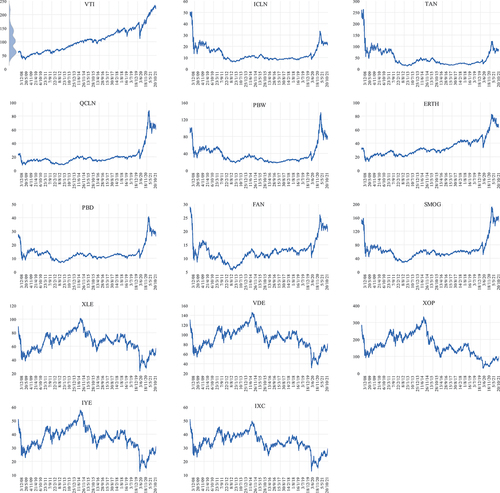
Table 3. Descriptive statistics for daily returns (30 June 2008–19 October 2021).

ETF returns	Mean	Std. Dev.	Skewness	Kurtosis	Jarque-Bera
Broad market ETFs:
ΔLn(VTIt)	0.00037	0.0129	−0.54	16.60	26907
ΔLn(SPYt)	0.00036	0.0128	−0.41	18.81	36267
Fossil fuel energy ETFs:
ΔLn(ICLNt)	−0.00022	0.0212	−0.69	14.64	19860
ΔLn(TANt)	−0.00030	0.0287	−0.42	9.87	6936
ΔLn(QCLNt)	0.00030	0.0212	−0.50	9.58	6417
ΔLn(PBWt)	−0.00006	0.0224	−0.49	9.40	6071
ΔLn(ERTHt)	0.00021	0.0166	−1.02	15.48	23113
ΔLn(PBDt)	0.00002	0.0189	−0.95	15.87	24494
ΔLn(FANt)	−0.00009	0.0174	−0.47	16.06	24800
ΔLn(SMOGt)	0.00001	0.0208	−0.61	14.63	19795
Fossil fuel energy ETFs:
ΔLn(XLEt)	−0.00012	0.0199	−0.77	18.66	35820
ΔLn(VDEt)	−0.00013	0.0201	−0.71	16.99	28601
ΔLn(XOPt)	−0.00027	0.0274	−1.39	31.15	115731
ΔLn(IYEt)	−0.00013	0.0199	−0.78	23.85	63229
ΔLn(IXCt)	−0.00015	0.0186	−0.77	19.49	39663
ΔLn(IEOt)	−0.00008	0.0240	−0.82	17.71	31691

Source: The Author’s calculations.

According to the Jarque-Bera statistics reported in Table 3, the normality assumption is rejected at the 1% significance level because all return series are negatively skewed and highly leptokurtic. Table 4 also shows the pairwise commonality (overlapping) matrix (using market caps as weights) between the constituents of all 13 ETFs. As expected, there is almost no overlapping between the eight renewable energy ETFs and the five fossil-fuel energy ETFs but the overlapping within each category of the ETFs appears to be high, particularly between the common holdings of VDE-XLE, IYE-XLE and IYE-VDE. A quick glance at Appendix 2 also shows that the top 15 companies within each fossil-fuel energy ETFs are highly similar.

Table 4. Overlapping matrix using market capitalizations as weights.

ETF	Renewable Energy ETFs								Fossil-fuel energy ETFs
	ICLN	TAN	QCLN	PBW	ERTH	PBD	FAN	SMOG	XLE	VDE	XOP	IYE	IXC
ICLN	1
TAN	0.26	1
QCLN	0.26	0.25	1
PBW	0.15	0.19	0.36	1
ERTH	0.28	0.15	0.30	0.15	1
PBD	0.26	0.23	0.24	0.34	0.18	1
FAN	0.37	0.01	0.00	0.01	0.10	0.14	1
SMOG	0.45	0.12	0.30	0.14	0.39	0.22	0.21	1
XLE	0.00	0.00	0.00	0.00	0.00	0.00	0.00	0.00	1
VDE	0.00	0.00	0.00	0.00	0.00	0.00	0.00	0.00	0.80	1
XOP	0.01	0.00	0.01	0.02	0.01	0.01	0.00	0.00	0.33	0.33	1
IYE	0.04	0.03	0.04	0.04	0.04	0.03	0.00	0.00	0.83	0.83	0.31	1
IXC	0.00	0.00	0.00	0.00	0.00	0.00	0.00	0.00	0.53	0.53	0.23	0.56	1

Similar to a correlation-matrix, the above symmetric and partitioned matrix shows the pairwise overlapping between the constituents of different ETFs using the corresponding market capitalization as weights.

Source: www.etfrc.com as of 19 October 2021.

V. Results and discussion

Table 5 presents the results of the ADF (augmented Dickey and Fuller 1979) test and PP (Phillips and Perron 1988) test, in which the lowest value of the Schwarz information criterion (SIC) was used as a guide to determine the optimum lag length or bandwidth. As expected, the corresponding null hypothesis is rejected at the 1% level for all 16 daily return series [or ΔLn(Y_t)=Ln(Y_t/Y_t−1))]. One can thus conclude that all return series are stationary and hence shocks can only temporarily influence the series. According to Figure 1, VTI exhibited an overall upward trend throughout the sample period (with the exception of a sharp fall due to the outbreak of COVID-19 in March 2020), whereas almost all eight renewable energy ETFs were stagnant before 2020 but rose substantially during March 2020-January 2021 and falling since then. However, unlike renewable energy ETFs, the graphs at the bottom two rows of Figure 1 indicate that the prices of five fossil-fuel energy ETFs exhibit two overall upward trends during 2008–2014 and 2020-present and one downward trend during 2014–2020. As can be seen from the kernel density distribution appearing in top-left graph in Figure 1, VTI, which is a proxy for the entire US equity market, is skewed to the left with three distinctive modes. This clearly indicates that there are three disparate groups of observations, motivating us to use multi-regime breaking regressions in the estimation procedure.

Table 5. The unit root test results.

ETF daily returns	ADF		PP
	t ratio	Optimal lag length	Adj. t-Stat	Optimal bandwidth
Broad market ETFs:
ΔLn(VTIt)	−66.01***	0	−66.10***	7
ΔLn(SPYt)	−66.48***	0	−66.74***	6
Fossil fuel energy ETFs:
ΔLn(ICLNt)	−57.78***	0	−57.77***	12
ΔLn(TANt)	−55.70***	0	−55.69***	13
ΔLn(QCLNt)	−57.61***	0	−57.60***	17
ΔLn(PBWt)	−38.91***	1	−57.22***	10
ΔLn(ERTHt)	−59.06***	0	−59.11***	14
ΔLn(PBDt)	−39.65***	1	−61.02***	7
ΔLn(FANt)	−60.59***	0	−60.59***	10
ΔLn(SMOGt)	−59.47***	0	−59.51***	12
Fossil fuel energy ETFs:
ΔLn(XLEt)	−62.96***	0	−62.87***	13
ΔLn(VDEt)	−62.76***	0	−62.65***	14
ΔLn(XOPt)	−61.92***	0	−61.88***	13
ΔLn(IYEt)	−65.16***	0	−64.93***	14
ΔLn(IXCt)	−61.78***	0	−61.74***	7
ΔLn(IEOt)	−61.16***	0	−61.12***	10

*** indicates that the corresponding null hypothesis is rejected at the 1% level of significance. The SIC is used to determine the optimal lag length/bandwidth.

Using daily observations during the sample period (30 June 2008–19 October 2021), Table 6 presents the fixed or non-asymmetric betas for all energy ETFs, which are sorted in descending order from top to bottom based on their market capitalization. The estimated equations perform reasonably well in terms of goodness-of-fit statistics as ${\bar{R}}^2$ for both renewable and fossil-fuel energy ETFs is on average 0.625. As can be seen from DW statistics, the estimated equations appear to be free from the first order serial correlation and all of the estimated betas are significant at the 1% level. As expected, all of the estimated betas exceed unity, particularly for TAN (β = 1.537) and XOP (β = 1.510), suggesting that investing in both types of energy ETFs are riskier than investing in a broad-based and diversified ETF such as VTI. On average, the results show that in response to a 1% rise (or fall) in the US stock market [proxied by ΔLn(VTI_t)], both renewable and fossil-fuel energy ETFs increase (decrease) by almost the same magnitude (i.e. 1.28%). However, as substantiated later in this section, the constant (non-asymmetric) betas in Table 6 can be very misleading because the upside and downside betas for renewable and fossil-fuel energy ETFs can significantly vary, particularly when the market is subject to a high degree of uncertainty.

Table 6. Unconditional betas for renewable and non-renewable energy ETFs $r_{\mathit{it}}={\alpha }_i+{\beta }_i{r}_{\mathit{Mt}}+{\epsilon }_{\mathit{it}}$.

ETFs	Intercept	β	Adj R^2	Overall F	AIC	SIC	HQC	DW
Renewable energy:
ICLN	−.001***	1.248***	0.573	4658	−5.7215	−5.7180	−5.7202	1.96
TAN	−.001**	1.537***	0.474	3131	−4.9066	−4.9031	−4.9054	1.87
QCLN	.000	1.325***	0.646	6339	−5.9087	−5.9052	−5.9074	2.04
PBW	−.001**	1.394***	0.640	6165	−5.7804	−5.7769	−5.7791	1.94
ERTH	.000	1.120***	0.748	10319	−6.7322	−6.7287	−6.7310	2.16
PBD	.000**	1.213***	0.679	7345	−6.2334	−6.2298	−6.2321	2.07
FAN	.000***	1.074***	0.627	5831	−6.2452	−6.2417	−6.2440	2.05
SMOG	.000**	1.329***	0.672	7110	−6.0180	−6.0145	−6.0167	2.05
Average		1.28	0.63
Fossil fuel energy:
XLE	−.001***	1.241***	0.642	6237	−6.0238	−6.0203	−6.0226	1.98
VDE	−.001***	1.251***	0.643	6259	−6.0110	−6.0074	−6.0097	1.95
XOP	−.001**	1.510***	0.504	3525	−5.0603	−5.0567	−5.0590	2.07
IYE	−.001***	1.229***	0.627	5844	−5.9782	−5.9747	−5.9769	2.06
IXC	−.001***	1.182***	0.666	6925	−6.2252	−6.2217	−6.2240	1.84
Average		1.28	0.62

Source: The Author’s estimation.

Table 7 relaxes the fixity assumption of betas for upside and downside markets. Once again, all the estimated upside and downside beta coefficients exceed unity and are statistically significant at the 1% level and as before there is no evidence of serial correlation. The downside betas for both renewable and fossil-fuel energy ETFs are greater than their corresponding upside betas. This means that both categories of energy ETFs tend to fall in downside markets more than they rise in upside markets. The highest downside betas are observed for TAN (1.657) and XOP (1.557). Note that these two ETFs also have the highest overall (non-asymmetric) betas in Table 6. However, based on the average betas shown in Table 7, in comparison with the fossil-fuel energy ETFs, it seems that renewable energy ETFs (especially those capturing a less diversified segment of renewables such as TAN and PBW) can have relatively larger downside and smaller upside betas.

Table 7. Estimated downside and upside beta coefficients. $r_{\mathit{it}}={\alpha }_i+{\epsilon }_{\mathit{it}}+\left\{\begin{array}{c}{\beta }_i^{-}{r}_{\mathit{Mt}}\mathrm{if}\mathrm{\Delta }{\mathrm{M}}_{\mathrm{t}}<0\\ {\beta }_i^{+}{r}_{\mathit{Mt}}\mathrm{if}\mathrm{\Delta }{\mathrm{M}}_{\mathrm{t}}\ge 0\end{array}\right.$

ETFs	Intercept	Upside beta β^+	Downside beta β^–	${\bar{R}}^2$	AIC	SIC	HQC	DW	Wald test F(1, 3469) H0: β^+=β^– H1: β^+<β^–
Renewable energy:
ICLN	.0002	1.121***	1.354***	0.576	−5.7281	−5.7228	−5.7262	1.96	24.96***
TAN	.0004	1.359***	1.687***	0.477	−4.9124	−4.9070	−4.9105	1.87	21.96***
QCLN	.0005*	1.233***	1.403***	0.648	−5.9128	−5.9075	−5.9109	2.04	16.14***
PBW	.0002	1.285***	1.484***	0.642	−5.7854	−5.7801	−5.7835	1.94	19.38***
ERTH	.0004**	1.040***	1.188***	0.750	−6.7396	−6.7343	−6.7377	2.16	27.77***
PBD	.0005**	1.089***	1.316***	0.683	−6.2442	−6.2389	−6.2423	2.07	39.93***
FAN	.0000	1.014***	1.125***	0.628	−6.2474	−6.2421	−6.2455	2.05	9.61***
SMOG	.0002	1.239***	1.404***	0.673	−6.0223	−6.0170	−6.0204	2.05	16.98***
Average betas		1.17	1.37
Fossil-fuel energy:
XLE	−.0002	1.189***	1.285***	0.643	−6.0249	−6.0196	−6.0230	1.98	5.73**
VDE	−.0002	1.192***	1.300***	0.644	−6.0125	−6.0072	−6.0106	1.95	7.16***
XOP	−.0004	1.455***	1.557***	0.504	−5.0604	−5.0551	−5.0585	2.07	2.47
IYE	−.0004*	1.207***	1.247***	0.627	−5.9779	−5.9726	−5.9760	2.06	0.93
IXC	−.0002	1.132***	1.225***	0.667	−6.2265	−6.2212	−6.2246	1.84	6.5**
Average betas		1.24	1.32

*, ** and *** indicate that the corresponding null hypothesis is rejected at the 10%, 5% and 1%, respectively.

It also seems that compared to renewables energy ETFs, the fossil-fuel energy ETFs on average have higher upside betas (1.24 versus 1.17). For example, according to Table 7, when the whole US market rises by 1%, ICLN and XLE increase by 1.121% and 1.189%, respectively, whereas when the market falls by the same magnitude the corresponding drawdowns are 1.354% and 1.285%. One can reach the same conclusion by comparing the upside and downside beta coefficients for both renewable and fossil-fuel energy ETFs, suggesting that all energy ETFs appearing in Table 7 rise much more slowly during market rallies than they fall during market selloffs.

Comparing the two-model selection criteria shown in Tables 6 and 7 pairwise, namely AIC (Akaike information criterion) and Hannan-Quinn criterion (HQC), reveals that the asymmetric model outperforms the fixed beta model for all ETFs. The use of SIC can lead to mixed results albeit still favouring the use of asymmetric model for most ETFs. The Wald test results also reject the null hypothesis of $H_0^{\hspace{0.17em}}:{\beta }^{+}={\beta }^{-}\mathrm{vs}{.\mathrm{H}}_1^{\hspace{0.17em}}:{\beta }^{+}{\beta }^{-}$at the 5% level of significance for 11 out of 13 ETFs in Table 7. It is thus statistically justifiable to distinguish between the upside and downside beta coefficients. All in all, the pairwise comparison of the estimated upside and downside betas for renewable and non-renewable energy ETFs in Table 7 suggest that both renewable and non-renewable energy ETFs tend to sustain large drawdowns during market selloffs and enjoy relatively less gains when market rallies.

Will these inferences change if uncertainty is incorporated into the model? To answer this question, using Equation (6)(6) $r_{\mathit{it}}=\sum _{\mathit{j}=1}^{\mathit{n}=2}{1}_i(\mathit{\tau },\mathrm{\Delta }\mathrm{VI}{\mathrm{X}}_{\mathrm{t}-\mathrm{d}})\cdot \left({\alpha }_{\mathit{ji}}+{\beta }_{ji}^{-}{r}_{\mathit{Mt}}+{\beta }_{ji}^{+}{r}_{\mathit{Mt}}\right)+{\epsilon }_{\mathit{it}}$(6) this study goes one step further by estimating the upside and downside beta coefficients in two distinct regimes based on optimized variations in the VIX index: Regime 1 (low uncertainty) and Regime 2 (high uncertainty). As can be seen from the results presented in Table 8, the upside and downside betas for each ETF are allowed to vary depending on the endogenously determined optimum changes in the VIX index. Based on the three model selection criteria, the estimated equations in Table 8 consistently outperform those in both Tables 6 and 7. This finding is not surprising as there is ample evidence that uncertainty in general can influence most financial and economic indicators (Wensheng, Ratti, and Vespignani 2017). Thus, it statistically makes sense to incorporate fear or uncertainty in the estimated equations in Table 8.

Table 8. Estimated downside and upside betas influenced by market uncertainty:$r_{\mathit{it}}={\alpha }_i+{\epsilon }_{\mathit{it}}+\left\{\begin{array}{c}\left.\left\{\begin{array}{c}{\beta }_{1i}^{-}{r}_{\mathit{Mt}}\mathrm{if}\mathrm{\Delta }{\mathrm{M}}_t<0\\ {\beta }_{1i}^{+}{r}_{\mathit{Mt}}\mathrm{if}\mathrm{\Delta }{\mathrm{M}}_t\ge 0\end{array}\right.\right\}\mathrm{if}\mathrm{\Delta }\mathrm{VI}{\mathrm{X}}_{\mathrm{t}-\mathrm{j}}<\mathit{\hspace{0.17em}}\mathit{\tau }\\ \left.\left\{\begin{array}{c}{\beta }_{2i}^{-}{r}_{\mathit{Mt}}\mathrm{if}\mathrm{\Delta }{\mathrm{M}}_t<0\\ {\beta }_{2i}^{+}{r}_{\mathit{Mt}}\mathrm{if}\mathrm{\Delta }{\mathrm{M}}_t\ge 0\end{array}\right.\right\}\mathrm{if}\mathrm{\Delta }\mathrm{VI}{\mathrm{X}}_{\mathrm{t}-\mathrm{j}}\ge \mathit{\tau }\end{array}\right.$

ETFs	Regime 1: less uncertainty: ΔVIXt-j <$\hat{\tau }$				Regime 2: high uncertainty: ΔVIXt-j ≥$\hat{\tau }$				$\hat{\tau }$	j	${\bar{R}}^2$	AIC	SIC	HQC	DW	Wald test: F(1, 3128)
	n1	α1	Upside${\beta }_{1i}^{+}$	Downside${\beta }_{1i}^{-}$	n2	α2	Upside${\beta }_{2i}^{+}$	Downside${\beta }_{2i}^{-}$								${\beta }_1^{+}={\beta }_2^{+}$	${\beta }_1^{-}={\beta }_2^{-}$
Renewable:
ICLN	471	0.0016**	1.001***	0.601***	2663	−0.0004	1.131***	1.193***	−0.850	0	0.552	−6.1479	−6.1363	−6.1437	1.92	2.57*	9.69***
TAN	471	0.0038***	1.124***	0.679**	2663	−0.0009*	1.569***	1.496***	−0.850	0	0.410	−5.1078	−5.0962	−5.1036	1.87	10.62***	6.50**
QCLN	471	0.0035***	1.044***	0.699***	2663	−0.0006*	1.528***	1.347***	−0.850	0	0.607	−6.0812	−6.0696	−6.0770	2.04	33.36***	10.82***
PBW	471	0.0024**	1.132***	0.646***	2663	−0.0005	1.477***	1.449***	−0.860	0	0.585	−5.9050	−5.8934	−5.9008	1.94	14.30***	13.88***
ERTH	1912	0.0002	1.152***	1.134***	1221	−0.0001	0.926***	1.120***	0.050	1	0.741	−7.0903	−7.0787	−7.0861	2.09	31.02***	0.15
PBD	471	0.0013*	1.002***	0.192	2663	0.0000	1.109***	1.237***	−0.850	0	0.650	−6.5425	−6.5309	−6.5383	2.03	2.59*	44.65***
FAN	2310	−0.0002	0.939***	0.715***	824	−0.0008*	1.224***	1.013***	0.350	0	0.587	−6.5977	−6.5861	−6.5936	2.01	3.58**	10.94***
SMOG	2658	−0.0006**	1.321***	1.212***	475	0.0016***	0.815***	1.302***	0.850	1	0.652	−6.4578	−6.4462	−6.4536	2.04	68.13***	2.76*
Average			1.09	0.74			1.22	1.270
Fossil-fuel:
XLE	2644	−0.0009***	1.251***	1.159***	489	0.0015**	1.060***	1.481***	0.800	1	0.592	−6.1726	−6.1610	−6.1684	1.95	7.56***	26.93***
VDE	2644	−0.0009***	1.255***	1.163***	489	0.0016**	1.028***	1.474***	0.800	1	0.581	−6.1333	−6.1217	−6.1291	1.95	10.24***	24.20***
XOP	2647	−0.0016***	1.548***	1.317***	486	0.0025**	1.407***	2.066***	0.820	1	0.446	−5.1376	−5.1260	−5.1334	2.07	1.42	51.54***
IYE	2644	−0.0009**	1.241***	1.155***	489	0.0020***	1.021***	1.490***	0.800	1	0.585	−6.1586	−6.1470	−6.1544	1.99	9.84***	28.60***
IXC	2644	−0.0008**	1.185***	1.115***	489	0.0020***	0.946***	1.458***	0.800	1	0.616	−6.3661	−6.3545	−6.3619	1.82	14.34***	37.97***
Average			1.30	1.18			1.09	1.59

*, ** and *** indicate that the corresponding null hypothesis is rejected at the 10%, 5% and 1% level, respectively. j in ΔVIX_t-j denotes the decay parameter.

Given 3134 daily variations in the VIX index during the sample period, the five largest renewable energy ETFs (namely ICLN, TAN, QCLN, PBW and PBD) lie in Regime 1 (low uncertainty) for only 471 days and 2663 days in Regime 2 (high uncertainty). The results show that it is more likely that the majority of renewable energy ETFs (particularly those with the largest AUM) to be in Regime 2, whereas the opposite is true for fossil-fuel energy ETFs. According to Table 8, all five fossil-fuel energy ETFs were in Regime 1 for 2647 days out of 3134 days or 84% of the times. As an example, when the market is characterized as highly uncertain (Regime 2), a 1% rise in the market leads to an upside beta of 1.131% for ICLN and only 1.060% for XLE. The corresponding downside betas for ICLN and XLE in Regime 2 were 1.193 and 1.481. It is interesting that the threshold parameter (τ) for most of renewable energy ETFs is around −0.85 whereas this estimate for the fossil-fuel ETFs is around + 0.80. Overall, this may suggest that a larger negative change in the VIX index is required for renewable energy ETFs to switch from Regime 2 to Regime 1. This means investors in renewables might be highly risk averse or skittish.

It is interesting to note that in Regime 2 the upside betas for TAN, QCLN, PBW, FAN are higher than the downside betas, whereas without any exception in Regime 2 the downside betas for all five fossil-fuel energy ETFs are greater than the upside market. Based on these results, one can conclude that when the market is highly uncertain, fossil-fuel energy ETFs become less desirable because they fall more during market pullbacks than they rise during market rallies. Although in Regime 2 the average downside beta is greater than the average upside beta, this asymmetry is much more severe in the context of fossil-fuel energy ETFs. Furthermore, in Regime 1 when the market becomes less uncertain, on average renewable energy ETFs have much lower downside betas than that of the fossil-fuel ETFs. The Wald test results in Table 8 clearly indicate that pairwise both null hypotheses (i.e.${\beta }_1^{+}={\beta }_2^{+}$ and ${\beta }_1^{-}={\beta }_2^{-}$) are rejected at the 1% level for all 13 ETFs except for ${\beta }_1^{+}={\beta }_2^{+}$in the case of XOP. Therefore, it can be concluded that when the market becomes very fearful fossil-fuel energy ETFs (which are also more likely to remain in Regime 1) tend to exhibit more drawdowns compared with their renewable counterparts.

The rest of this section compares the relative performance of investing in renewable energy ETFs with the opportunities in the other sectors of the economy (e.g. tech, health, finance etc.). Table 9 presents three risk and reward ratios (Sharpe, Sortino and Treynor) in the last five and 10 years for both renewable and non-renewable energy ETFs as well as the major sectoral ETFs in the US. This table is sorted in descending order using the average Sharpe ratio during the last 5 years within each subheading. As can be seen, with the exception of XLK, all Sharpe ratios in the last five years are below unity. When the five-year Sharpe ratio of a given ETF is less than that of the top three renewable energy ETFs (i.e. TAN, QCLN and ICLN), the relevant Sharpe ratio in Table 9 is shown in bold. To facilitate pairwise comparisons, the top-three renewable energy ETFs are in italic.

Table 9. Risk and reward ratios in different trailing periods.

ETFs	5 years			10 years
	Treynor	Sharpe	Sortino	Treynor	Sharpe	Sortino
Total market VTI	11.5	0.79	1.21	12.27	0.92	1.43
S&P500: SPY	12.5	1.52	0.96	12.96	0.96	1.52
Sector:
Information Technology: XLK	19.78	1.03	1.75	17.61	1.11	1.91
Health Care: XLV	16.02	0.94	1.77	18.47	1.06	1.84
Consumer Staples: XLP	15.2	0.92	1.68	18.97	0.93	1.56
Real Estate: XLRE	14.14	0.70	1.07	na	na	na
Consumer Discretionary: XLY	10.86	0.69	1.09	13.25	0.90	1.48
Utilities: XLU	20.62	0.64	1.02	27.67	0.76	1.2
Materials: XLB	10.14	0.64	1.00	9.43	0.67	1.06
Industrials: XLI	7.00	0.49	0.72	10.53	0.74	1.13
Financials: XLF	7.57	0.47	0.68	11.01	0.73	1.11
Energy: XLE	3.99	0.34	0.53	2.61	0.27	0.41
Communication Services: XTL	3.39	0.30	0.45	7.62	0.51	0.77
Renewable energy:
TAN	19.58	0.85	1.51	7.86	0.50	0.86
QCLN	15.47	0.81	1.48	11.79	0.71	1.26
ICLN	15.46	0.72	1.23	8.08	0.51	0.81
SMOG	11.69	0.68	1.22	10.38	0.68	1.18
PBW	11.89	0.65	1.12	5.40	0.41	0.68
PBD	9.86	0.58	0.99	7.84	0.54	0.88
ERTH	8.60	0.56	0.89	8.73	0.63	1.01
FAN	8.16	0.48	0.77	10.84	0.68	1.10
Fossil-fuel energy ETFs
IEO	4.59	0.41	0.65	2.15	0.28	0.43
XLE	3.99	0.34	0.53	2.61	0.27	0.41
VDE	3.30	0.32	0.49	1.81	0.23	0.35
IXC	4.09	0.32	0.48	1.62	0.2	0.3
IYE	2.94	0.30	0.46	1.62	0.22	0.33
XOP	−0.32	0.24	0.39	−2.29	0.10	0.15

All the above measures were extracted from www.morningstar.com.au on 20 May 2022 and then sorted in descending order using the five-year Sharpe ratio. When the five-year Sharpe ratio of a given ETF is less than that of the top three renewable energy ETFs (i. e. TAN, QCLN and ICLN), the relevant Sharpe ratio is shown in bold. The top-three renewable energy ETFs are in italic.

The inferences based on the results in Table 8 are also consistent with the three risk and reward statistics in Table 9.¹ According to Table 9, regardless of which measure of risk and reward statistics and trailing period are taken into account, all eight renewable energy ETFs outperform each and every fossil-fuel energy ETF. For instance, let us consider the pairwise comparison between the top three renewable energy ETFs. As can be seen in the last 5 years, the Sharpe, Sortino and Treynor ratios for TAN (0.85, 1.51, 19.58, respectively), QCLN (0.81, 1.48, 15.47) and ICLN (0.72, 1.23, 15.46) are conspicuously higher than those for IEO (0.41, 0.65, 4.59), XLE (0.34, 0.53, 3.39) and VDE (0.32, 0.49, 3.30). The same inference could be made if the ten-year trailing period was taken into consideration.

It is interesting to note that based on the last five-year Sharpe and Sortino ratios presented in Table 9, TAN and QCLN outperform the total market (VTI) as well as the following eight sectoral ETFs: real estate (XLRE), consumer discretionary (XLY), utilities (XLU), materials (XLB), industrials (XLI), financials (XLF), energy (XLE) and communication services (XTL). It should also be noted that if we use the ten-year trailing period in lieu of the five-year period, these inferences will change. This is not surprising as investing in renewables has been gathering steam and becoming increasingly popular in more recent years. In terms of downside risk, the top three renewable energy ETFs in Table 9 are even capable of outperforming eight out of eleven well-established sectoral ETFs (see the average Sortino ratios during the last five years).

Overall, there is a strong business case for investing in renewables, particularly during the last 5 years. In conclusion, the results in Tables 8 and 9 clearly support the view that investing in renewable energy ETFs are not only good for the environment but also compared to major sectoral ETFs (including fossil fuels) they provide relatively better risk-adjusted returns. Our findings are also broadly consistent with a number of studies examining renewable and non-renewable ETFs (Alexopoulos 2018; Miralles-Quirós and Mar Miralles-Quirós 2019). Based on a comprehensive analysis of the out-of-sample performance of different portfolio strategies using the returns and volatility forecasts, Miralles-Quirós and Mar Miralles-Quirós (2019) find that renewable energy ETFs are a real alternative for investors as they clearly outperform non-renewable energy ETFs. Alexopoulos (2018, 105) in a comparative study of conventional and clean ETFs also state that ‘a portfolio including clean and conventional ETFs in aggregate, performs better in terms of higher returns and lower risk than two disaggregated portfolios with clean and conventional ETFs separately’.

Furthermore, renewable energy ETFs can provide diversification benefits (Monaca, Sarah, and Byrne 2018) and to achieve these benefits, Dragomirescu-Gaina, Galariotis, and Philippas (2021) assert that political and regulatory authorities should reduce policy uncertainty and incentivize the use of green products as an integral part of critical infrastructure through a set of consistent and coordinated policies. As for the implementation of such policies, Sadorsky (2012) argues that renewable energy risk rises when the price of oil goes up or when renewable sales dwindle. Therefore, to encourage the use of renewables, state and federal governments should impose production and consumption taxes on fossil fuels to support financing investable activities of renewable energy companies.

VI. Conclusion remarks

Capturing the asymmetry between upside and downside co-movements has important implications for portfolio selection and risk management strategies. This paper examines the performance of two categories of energy ETFs (renewable vs. fossil-fuel) and how their upside and downside betas interact with market uncertainty. The sample period (30 June 2008–19 October 2021) includes daily observations for the eight largest renewable energy ETFs (i.e. ICLN, TAN, QCLN, PBW, ERTH, PBD, FAN and SMOG) and five major fossil-fuel energy ETFs (i.e. XLE, VDE, XOP, IYE, and IXC). The choice of the sample period and ETFs was solely influenced by data availability. The market is proxied with an ETF known as VTI, which includes all 3870 companies listed in the US. An initial comparative analysis of the beta coefficients indicates that the difference between the upside and downside beta coefficients are statistically significant, whereby both renewable and fossil-fuel energy ETFs tend to fall more than they rise in response to negative and positive changes in the market. The results hence confirm that for energy ETFs fear in market selloffs is more contagious than optimism in market rallies.

This paper, then, goes one step further and proposes a composite threshold model in which the upside and downside coefficients are moderated by optimal variations in the VIX index, which is a well-known measure of market uncertainty. The proposed model differentiates between upside and downside betas when the market is subject to varying degrees of uncertainty with two distinct regimes: Regime 1 (low uncertainty) and Regime 2 (high uncertainty). This study shows that asymmetric betas without incorporating uncertainty in the estimation process can lead to misleading inferences and mask important differences between the two categories of ETFs. It is found that when the market is highly uncertain, fossil-fuel energy ETFs become less desirable. The findings of this paper are also consistent with three well-known measures of risk and reward (i.e. Sharpe, Sortino and Treynor) as all renewable energy ETFs outperform fossil-fuel energy ETFs irrespective of which trailing period is taken into consideration.

The results in this study support the view that during the last 5 years some renewable energy ETFs are even capable of outperforming the following sectoral ETFs in terms Sharpe and Sortino ratios: real estate (XLRE), consumer discretionary (XLY), utilities (XLU), materials (XLB), industrials (XLI), financials (XLF), energy (XLE) and communication services (XTL). Based on these findings, renewable energy ETFs have great potential to generate high returns, but the risk associated with renewables should further be mitigated by government. To achieve this, government and regulatory authorities should create a sustainable demand for renewable energy through implementing direct green procurement strategies or via incentivizing the use of renewables in both domestic and foreign markets. This may involve the use of feed in tariffs, green rebates and subsidies. In conclusion, based on the findings in this paper, there is a more favourable business case for investing in renewables than common perception would suggest.

Future research should be extended to compare and contrast the interplay between market uncertainty (proxied by both the VIX index and the CNN’s fear and greed index) and extreme downside betas across different sectoral ETFs (i.e. energy as well as non-energy ETFs such as XLB, XLF, XLK etc). In order to make robust inferences regarding the moderating effect of market uncertainty on upside and downside betas, one can also adopt Markov regime switching models in which the VIX index or the CNN’s fear and greed index can separately appear as a probability regressor. Furthermore, future research can investigate how changes in oil and gas prices influencing the sectoral rotation by investors”.

Acknowledgments

I would like to thank two anonymous referees, whose useful feedback considerably improved an earlier version of this article. The usual caveat applies.

Disclosure statement

No potential conflict of interest was reported by the author(s).

Notes

¹ As a rule of thumb, the higher the three ratios (i.e. Sharpe, Sortino or Treynor), the more desirable a portfolio.

Appendix

Table

No	ICAN	%	TAN	%	QCLN	%	PBW	%
1	Enphase Energy, Inc	8.69	Enphase Energy, Inc.	12.42	Tesla Inc	10.17	Standard Lithium Ltd.	2.10
2	Vestas Wind Systems A/S	8.08	SolarEdge Technologies, Inc.	11.20	Enphase Energy, Inc.	7.49	SunPower Corporation	2.01
3	Plug Power Inc.	5.52	Sunrun Inc.	7.21	NIO Inc. Sponsored ADR Class A	7.21	Bloom Energy Corporation Class A	2.00
4	Orsted	5.48	First Solar, Inc.	7.01	Albemarle Corporation	7.14	Tesla Inc	1.93
5	SolarEdge Technologies, Inc.	5.28	Xinyi Solar Holdings Ltd.	6.10	ON Semiconductor Corporation	5.03	Enovix Corporation	1.86
6	Consolidated Edison, Inc.	5.11	Daqo New Energy Corp Sponsored ADR	3.89	Plug Power Inc.	4.95	Plug Power Inc.	1.84
7	Iberdrola SA	3.93	SunPower Corporation	3.2	SolarEdge Technologies, Inc.	4.21	Enphase Energy, Inc.	1.8
8	EDP-Energias de Portugal SA	3.66	Sunnova Energy International Inc	3.18	XPeng, Inc. ADR Sponsored Class A	3.78	Wolfspeed Inc	1.8
9	SSE plc	3.51	Shoals Technologies Group, Inc. Class A	3.14	Wolfspeed Inc	3.55	Renewable Energy Group, Inc.	1.78
10	First Solar, Inc.	3.35	Hannon Armstrong Sustainable Infrastructure	2.74	First Solar, Inc.	3.18	ReneSola Ltd. Sponsored ADR	1.73
11	Sunrun Inc.	3.32	Array Technologies Inc	2.72	Sunrun Inc.	2.92	Sunrun Inc.	1.72
12	Xinyi Solar Holdings Ltd.	2.70	JinkoSolar Holding Co., Ltd. Sponsored ADR	2.66	Brookfield Renewable Partners LP	2.81	Sunnova Energy International Inc	1.71
13	EDP Renovaveis SA	2.00	Atlantica Sustainable Infrastructure plc	2.61	Universal Display Corporation	2.15	FuelCell Energy, Inc.	1.70
14	Siemens Gamesa Renewable Energy	1.78	Encavis AG	2.22	Acuity Brands, Inc.	1.88	American Superconductor Corporation	1.60
15	Siemens Energy AG	1.69	Canadian Solar Inc.	2.21	ChargePoint Holdings, Inc. Class A	1.88	Lithium Americas Corp.	1.60
	Total top 15	64.1		72.51		68.35		27.18
No	ERTH	%	PBD	%	FAN	%	SMOG	%
1	Tesla Inc	7.11	Plug Power Inc.	1.21	Vestas Wind Systems A/S	8.53	Tesla Inc	11.43
2	Vestas Wind Systems A/S	5.00	Bloom Energy Corporation Class A	1.20	China Longyuan Power Group Corp. Ltd. H	7.46	NextEra Energy, Inc.	7.06
3	NIO Inc. Sponsored ADR A	5.00	SunPower Corporation	1.12	Orsted	7.26	Iberdrola SA	6.10
4	Enphase Energy, Inc.	4.72	FuelCell Energy, Inc.	1.11	Northland Power Inc.	6.69	NIO Inc. Sponsored ADR A	5.72
5	Digital Realty Trust, Inc.	4.37	Enphase Energy, Inc.	1.11	Siemens Gamesa Renewable Energy, S.A.	5.84	Enel SpA	5.51
6	Central Japan Railway Company	3.49	Wolfspeed Inc	1.08	EDP Renovaveis SA	4.27	Vestas Wind Systems A/S	5.31
7	Plug Power Inc.	3.10	Li-Cycle Holdings Corp.	1.08	Boralex Inc. Class A	3.07	Samsung SDI Co., Ltd	3.98
8	SolarEdge Technologies, Inc.	2.98	NEL ASA	1.07	Innergex Renewable Energy Inc.	2.40	Orsted	3.85
9	Li Auto, Inc. Sponsored ADR A	2.94	American Superconductor Corporation	1.06	Nordex SE	2.30	Enphase Energy, Inc.	3.60
10	XPeng, Inc. ADR Sponsored A	2.90	QuantumScape Corporation A	1.04	EDP-Energias de Portugal SA	2.10	XPeng, Inc. ADR Sponsored A	3.43
11	Kingspan Group Plc	2.86	2G Energy AG	0.99	NextEra Energy, Inc.	2.02	BYD Company Limited Class H	3.37
12	Darling Ingredients Inc.	2.24	Renewable Energy Group, Inc.	0.98	SSE plc	2.02	Lucid Group, Inc.	3.07
13	Contemporary Amperex Technology Co.	2.16	Sunrun Inc.	0.98	Prysmian S.p.A.	2.01	NIBE Industrier AB Class B	3.04
14	Umicore	1.89	EVgo, Inc. Class A	0.96	General Electric Company	1.99	Li Auto, Inc. Sponsored ADR A	2.81
15	Alstom SA	1.86	United Renewable Energy Co., Ltd.	0.96	ENGIE SA.	1.99	Plug Power Inc.	2.52
	Total top 15 holdings	52.62		15.95		59.95		70.80

Source: www.etf.com as of 4 November 2021.

Appendix

Table

No	XLE	%	VDE	%	XOP	%	IYE	%	IXC	%
1	Exxon Mobil	22.44	Exxon Mobil	20.77	SM Energy	3.49	Exxon Mobil	20.32	Exxon Mobil	13.48
2	Chevron	19.85	Chevron	16.76	Callon Petroleum	3.13	Chevron	16.55	Chevron	10.94
3	Schlumberger NV	4.66	ConocoPhillips	6.33	Marathon Oil	2.86	ConocoPhillips	7.75	TotalEnergies SE	6.14
4	EOG Resources, Inc.	4.62	EOG Resources, Inc.	3.66	Devon Energy	2.83	EOG Resources, Inc.	5.05	ConocoPhillips	4.93
5	ConocoPhillips	4.48	Schlumberger NV	3.62	Diamondback Energy, Inc.	2.81	Schlumberger NV	4.17	BP p.l.c.	4.81
6	Pioneer Natural Resources	4.38	Marathon Petroleum	3.61	Renewable Energy Group	2.77	Marathon Petroleum	3.86	Royal Dutch Shell Plc Class A	4.64
7	Marathon Petroleum	4.32	Pioneer Natural Resources	3.14	APA Corp.	2.75	Pioneer Natural Resources	3.53	Royal Dutch Shell Plc Class B	4.20
8	Williams Companies, Inc.	3.52	Kinder Morgan Inc Class P	3.08	Occidental Petroleum	2.64	Williams Companies, Inc.	2.95	Enbridge Inc.	4.19
9	Phillips 66	3.47	Phillips 66	2.91	EOG Resources, Inc.	2.63	Kinder Morgan Inc Class P	2.85	EOG Resources, Inc.	2.67
10	Kinder Morgan Inc Class P	3.45	Williams Companies, Inc.	2.78	Ovintiv Inc	2.56	Phillips 66	2.80	TC Energy Corporation	2.62
11	Valero Energy	3.29	Valero Energy	2.54	PBF Energy, Inc. Class A	2.56	Valero Energy	2.57	Canadian Natural Resources	2.49
12	Occidental Petroleum	3.02	Occidental Petroleum	2.21	Murphy Oil	2.54	Enphase Energy, Inc.	2.41	Schlumberger NV	2.23
13	ONEOK, Inc.	2.97	ONEOK, Inc.	2.15	ConocoPhillips	2.53	Occidental Petroleum	2.24	Pioneer Natural Resources	2.10
14	Devon Energy	2.55	Cheniere Energy, Inc.	1.79	Range Resources	2.53	ONEOK, Inc.	2.23	Marathon Petroleum	2.08
15	Hess Corporation	2.39	Devon Energy	1.73	Continental Resources, Inc.	2.44	Devon Energy	2.13	Suncor Energy Inc.	1.93
	Total top 15	89.41		77.08		41.07		81.41		69.45

Source: www.etf.com as of 4 November 2021.

References

- Agrrawal, P., and D. Waggle. 2010. “The Dispersion of ETF Betas on Financial Websites.” Journal of Investing 19 (1): 13–24. https://doi.org/10.3905/JOI.2010.19.1.013.
- Alexopoulos, T. A. 2018. “To Trust or Not to Trust? A Comparative Study of Conventional and Clean Energy Exchange-Traded Funds.” Energy Economics 72:97–107. https://doi.org/10.1016/j.eneco.2018.03.013.
- Andersson, M., P. Bolton, and F. Samama. 2016. “Hedging Climate Risk.” Financial Analysts Journal 72 (3): 13–32. https://doi.org/10.2469/faj.v72.n3.4.
- Ang, A., and J. Chen. 2002. “Asymmetric Correlations of Equity Portfolios.” Journal of Financial Economics 63 (3): 443–494. https://doi.org/10.1016/S0304-405X(02)00068-5.
- Ang, A., J. Chen, and Y. Xing. 2006. “Downside Risk.” The Review of Financial Studies 19 (4): 1191–1239. https://doi.org/10.1093/rfs/hhj035.
- Atilgan, Y., K. O. Demirtas, and A. D. Gunaydin. 2020. “Downside Beta and the Cross Section of Equity Returns: A Decade Later.” European Financial Management 26 (2): 316–347. https://doi.org/10.1111/eufm.12258.
- Auer, B. R., and F. Schuhmacher. 2013. “Robust Evidence on the Similarity of Sharpe Ratio and Drawdown-Based Hedge Fund Performance Rankings.” Journal of International Financial Markets, Institutions and Money 24:153–165. https://doi.org/10.1016/j.intfin.2012.11.010.
- Bae, K.-H., G. A. Karolyi, and R. M. Stulz. 2003. “A New Approach to Measuring Financial Contagion.” The Review of Financial Studies 16 (3): 717–763. https://doi.org/10.1093/rfs/hhg012.
- Bai, J., and P. Perron. 2003. “Computation and Analysis of Multiple Structural Change Models.” Journal of Applied Econometrics 18 (1): 1–22. https://doi.org/10.1002/jae.659.
- Bawa, V. S., and E. B. Lindenberg. 1977. “Capital Market Equilibrium in a Mean-Lower Partial Moment Framework.” Journal of Financial Economics 5 (2): 189–200. https://doi.org/10.1016/0304-405X(77)90017-4.
- Bekaert, G., and W. Guojun. 2000. “Asymmetric Volatility and Risk in Equity Markets.” The Review of Financial Studies 13 (1): 1–42. https://doi.org/10.1093/rfs/13.1.1.
- Chan, K.-S. 1993. “Consistency and Limiting Distribution of the Least Squares Estimator of a Threshold Autoregressive Model.” The Annals of Statistics 21 (1): 520–533. https://doi.org/10.1214/aos/1176349040.
- Chiang, K., M.-L. Lee, and C. Wisen. 2004. “Another Look at the Asymmetric Reit-Beta Puzzle.” Journal of Real Estate Research 26 (1): 25–42. https://doi.org/10.1080/10835547.2004.12091131.
- Christie, A. A. 1982. “The Stochastic Behavior of Common Stock Variances: Value, Leverage and Interest Rate Effects.” Journal of Financial Economics 10 (4): 407–432. https://doi.org/10.1016/0304-405X(82)90018-6.
- Chung, Y., P. Hyun, and A. Hong. 2019. “What Causes the Asymmetric Correlation in Stock Returns?” Journal of Empirical Finance 54:190–212. https://doi.org/10.1016/j.jempfin.2019.10.001.
- Dennis, S. A., P. Simlai, and W. Steven Smith. 2017. “Modified Beta and Cross-Sectional Stock Returns.” In Growing Presence of Real Options in Global Financial Markets, 75–104. Emerald Publishing Limited. https://doi.org/10.1108/S0196-382120170000033005.
- Dickey, D. A., and W. A. Fuller. 1979. “Distribution of the Estimators for Autoregressive Time Series with a Unit Root.” Journal of the American Statistical Association 74 (366a): 427–431. https://doi.org/10.1080/01621459.1979.10482531.
- Dragomirescu-Gaina, C., E. Galariotis, and D. Philippas. 2021. “Chasing the ‘Green bandwagon’ in Times of Uncertainty.” Energy Policy 151:112190. https://doi.org/10.1016/j.enpol.2021.112190.
- Eling, M. 2008. “Does the Measure Matter in the Mutual Fund Industry?” Financial Analysts Journal 64 (3): 54–66. https://doi.org/10.2469/faj.v64.n3.6.
- Eling, M., and F. Schuhmacher. 2007. “Does the Choice of Performance Measure Influence the Evaluation of Hedge Funds?” Journal of Banking and Finance 31 (9): 2632–2647. https://doi.org/10.1016/j.jbankfin.2006.09.015.
- Estrada, J. 2002. “Systematic Risk in Emerging Markets: The D-CAPM.” Emerging Markets Review 3 (4): 365–379. https://doi.org/10.1016/S1566-0141(02)00042-0.
- Estrada, J. 2006. “Downside Risk in Practice.” Journal of Applied Corporate Finance 18 (1): 117–125. https://doi.org/10.1111/j.1745-6622.2006.00080.x.
- Fishburn, P. C. 1977. “Mean-Risk Analysis with Risk Associated with Below-Target Returns.” American Economic Review 67 (2): 116–126.
- Fisher, J. D., and J. D’Alessandro. 2021. “Portfolio Upside and Downside Risk—Both Matter!” The Journal of Portfolio Management 47 (10): 158–171. https://doi.org/10.3905/jpm.2021.1.263.
- Forbes, W., E. Kiselev, and L. Skerratt. 2021. “The Stability and Downside Risk to Contrarian Profits: Evidence from the S&P 500.” International Journal of Finance & Economics 28 (1): 733–750. https://doi.org/10.1002/ijfe.2447).
- French, K. R., G. William Schwert, and R. F. Stambaugh. 1987. “Expected Stock Returns and Volatility.” Journal of Financial Economics 19 (1): 3–29. https://doi.org/10.1016/0304-405X(87)90026-2.
- Grobys, K., and T. Huhta-Halkola. 2019. “Combining Value and Momentum: Evidence from the Nordic Equity Market.” Applied Economics 51 (26): 2872–2884. https://doi.org/10.1080/00036846.2018.1558364.
- Han, Y., and L. Kong. 2022. “A Trend Factor in Commodity Futures Markets: Any Economic Gains from Using Information Over Investment Horizons?” Journal of Futures Markets 42 (5): 803–822. https://doi.org/10.1002/fut.22291.
- Hansen, B. E. 2011. “Threshold Autoregression in Economics.” Statistics and Its Interface 4 (2): 123–127. https://doi.org/10.4310/SII.2011.v4.n2.a4.
- Hong, Y., T. Jun, and G. Zhou. 2007. “Asymmetries in Stock Returns: Statistical Tests and Economic Evaluation.” The Review of Financial Studies 20 (5): 1547–1581. https://doi.org/10.1093/rfs/hhl037.
- Jiang, C., X. Ding, Q. Xu, X. Liu, and Y. Liu. 2019. “Portfolio Selection Based on Predictive Joint Return Distribution.” Applied Economics 51 (2): 196–206. https://doi.org/10.1080/00036846.2018.1494812.
- Karolyi, G. A., and R. M. Stulz. 1996. “Why Do Markets Move Together? An Investigation of Us‐Japan Stock Return Comovements.” The Journal of Finance 51 (3): 951–986. https://doi.org/10.1111/j.1540-6261.1996.tb02713.x.
- Kuang, W. 2022. “Is Hedge Fund a Hedge for Equity Markets?” Applied Economics 54 (27): 3154–3179. https://doi.org/10.1080/00036846.2021.2003748.
- Lahtinen, K. D., C. M. Lawrey, and K. J. Hunsader. 2018. “Beta Dispersion and Portfolio Returns.” Journal of Asset Management 19 (3): 156–161. https://doi.org/10.1057/s41260-017-0071-6.
- Liu, Q., S. Wang, and C. Sui. 2022. “Market Volatility, Market Skewness, and the Cross-Section of Expected Returns in Chinese Equity Markets.” Applied Economics 1–17. https://doi.org/10.1080/00036846.2022.2140766.
- Longin, F., and B. Solnik. 1995. “Is the Correlation in International Equity Returns Constant: 1960–1990?” Journal of International Money and Finance 14 (1): 3–26. https://doi.org/10.1016/0261-5606(94)00001-H.
- Markovitz, H. M. 1959. Portfolio Selection: Efficient Diversification of Investments. New York: John Wiley.
- Marti‐Ballester, C. 2020. “Examining the Behavior of Renewable‐Energy Fund Investors.” Business Strategy and the Environment 29 (6): 2624–2634. https://doi.org/10.1002/bse.2525.
- Miralles-Quirós, J. L., and M. Mar Miralles-Quirós. 2019. “Are Alternative Energies a Real Alternative for Investors?” Energy Economics 78:535–545. https://doi.org/10.1016/j.eneco.2018.12.008.
- Molyboga, M., and C. L’Ahelec. 2016. “Portfolio Management with Drawdown-Based Measures.” Journal of Alternative Investments 19 (3): 75–89. https://doi.org/10.3905/jai.2017.19.3.075.
- Monaca, L., M. A. Sarah, and J. Byrne. 2018. “Clean Energy Investing in Public Capital Markets: Portfolio Benefits of Yieldcos.” Energy Policy 121:383–393. https://doi.org/10.1016/j.enpol.2018.06.028.
- Nicholas, A., and J. E. Payne. 2012. “Renewable and Non-Renewable Energy Consumption-Growth Nexus: Evidence from a Panel Error Correction Model.” Energy Economics 34 (3): 733–738. https://doi.org/10.1016/j.eneco.2011.04.007.
- Pettengill, G. N., S. Sundaram, and I. Mathur. 1995. “The Conditional Relation Between Beta and Returns.” The Journal of Financial and Quantitative Analysis 30 (1): 101–116. https://doi.org/10.2307/2331255.
- Phillips, P. C., and P. Perron. 1988. “Testing for a Unit Root in Time Series Regression.” Biometrika 75 (2): 335–346. https://doi.org/10.1093/biomet/75.2.335.
- Polemis, M. L., and A. Spais. 2020. “Disentangling the Drivers of Renewable Energy Investments: The Role of Behavioral Factors.” Business Strategy and the Environment 29 (6): 2170–2180. https://doi.org/10.1002/bse.2493.
- Sadorsky, P. 2012. “Modeling Renewable Energy Company Risk.” Energy Policy 40:39–48. https://doi.org/10.1016/j.enpol.2010.06.064.
- Salim, R. A., K. Hassan, and S. Shafiei. 2014. “Renewable and Non-Renewable Energy Consumption and Economic Activities: Further Evidence from OECD Countries.” Energy Economics 44:350–360. https://doi.org/10.1016/j.eneco.2014.05.001.
- Schuhmacher, F., and M. Eling. 2011. “Sufficient Conditions for Expected Utility to Imply Drawdown-Based Performance Rankings.” Journal of Banking & Finance 35 (9): 2311–2318. https://doi.org/10.1016/j.jbankfin.2011.01.031.
- Sebastien, P., and R. A. Panariello. 2018. “When Diversification Fails.” Financial Analysts Journal 74 (3): 19–32. https://doi.org/10.2469/faj.v74.n3.3.
- Sharpe, W. F. 1964. “Capital Asset Prices: A Theory of Market Equilibrium Under Conditions of Risk.” The Journal of Finance 19 (3): 425–442. https://doi.org/10.1111/j.1540-6261.1964.tb02865.x.
- Sortino, F., and H. Forsey. 1996. “On the Use and Misuse of Downside Risk.” The Journal of Portfolio Management 22 (2): 35–42. https://doi.org/10.3905/jpm.1996.35.
- Sortino, F. A., and R. van der Meer. 1991. “Downside Risk.” The Journal of Portfolio Management 18 (2): 27–31. https://doi.org/10.3905/jpm.1991.409343.
- Treynor, J. L. 1965. “How to Rate Management Investment Funds.” Harvard Business Review 44 (1): 63–75.
- Valadkhani, A. 2022. “Do Large-Cap Exchange-Traded Funds Perform Better Than Their Small-Cap Counterparts in Extreme Market Conditions?” Global Finance Journal 53:100743. https://doi.org/10.1016/j.gfj.2022.100743.
- Wensheng, K., R. A. Ratti, and J. L. Vespignani. 2017. “Oil Price Shocks and Policy Uncertainty: New Evidence on the Effects of US and Non-US Oil Production.” Energy Economics 66:536–546. https://doi.org/10.1016/j.eneco.2017.01.027.
- Young, T. W. 1991. “Calmar Ratio: A Smoother Tool.” Futures 20 (1): 40.