Impact of public subsidies on persistent and transient technical efficiency: evidence from French mixed crop-livestock farms

ABSTRACT

This study contributes to the existing literature on the influence of public subsidies on farmers’ technical efficiency by highlighting the importance of separating persistent and transient inefficiency. Using data from a sample of French mixed (crop-livestock) farms, and relying on recent developments in stochastic frontier analysis, we find that public subsidies are positively associated with both persistent and transient technical inefficiency. The effect of public subsidies on persistent technical inefficiency suggests that they induce sluggish adjustments (restructuring) in farm management practices.

KEYWORDS:

• Persistent and transient technical efficiency
• endogeneity
• public subsidies
• mixed farms
• France

JEL CLASSIFICATION:

• Q12
• Q18
• C54
• D24

I. Introduction

There is a long tradition of government intervention in the agricultural sector, particularly in more developed countries, with the implementation of policies that provide financial support to farmers. For instance, agricultural support policies in the United States (US) and the European Union (EU) began in the 1930s and the 1960s, respectively. In the last two decades, the EU has spent around €50 billion annually on the Common Agricultural Policy (CAP), an amount that represents approximately 40% of the EU budget (Anania and Pupo D’Andrea 2015; Greer 2013). Similarly, the US Farm Bill costs around €65 billion annually and agricultural subsidies account for approximately 20% of this figure (Johnson 2007; Johnson and Monke 2014). Since their inception, agricultural support policies in developed countries have been subject to a continuous reform process to adapt to the changing economic, social and environmental conditions within which farmers operate. The major reforms of agricultural support policies have entailed a movement from market price support to coupled direct payments (production-related supports) and, more recently, decoupled direct payments to farmers. In the EU, along with the direct payment schemes, farmers have been encouraged to engage voluntarily in environmentally friendly farming practices through various agri-environmental schemes. All these payments are aimed mainly at supporting producer incomes, preserving strategic farming systems, and encouraging environmentally friendly practices. However, theoretical and empirical studies (e.g. Kumbhakar and Lien 2010; Martin and Page 1983; Minviel and Latruffe 2017; Serra, Zilberman, and Gil 2008; Zhu and Oude Lansink 2010) show that public subsidies may also influence the technical efficiency of farmers.

In the subsidy-efficiency literature, a number of papers have analysed the link between changes in agricultural support policies and the evolution of farm technical efficiency. One of the potential drawbacks of these papers is that they are almost exclusively based on overall technical efficiency measures that do not distinguish between transient and persistent inefficiency. This paper contributes to the literature on the subsidy-efficiency nexus by analysing the effects of public subsidies on both transient and persistent technical inefficiencies. In practice, persistent and transient inefficiencies are expected to have different policy implications. Indeed, transient (short-run) inefficiency can change, inter alia, because of farmers’ experience and their ability to handle random factors such as weather conditions or pest outbreaks (Kumbhakar, Lien, and Hardaker 2014; Manevska-Tasevska et al., 2017). In contrast, persistent inefficiency is by definition time-invariant, and thus can only change in the long run through farm restructuring. In other words, persistent inefficiency is unlikely to evolve unless there are major changes in drivers, such as public policies, which may affect farm management practices (Kumbhakar, Lien, and Hardaker 2014; Kumbhakar, Wang, and Horncastle 2015). Therefore, it is informative to separate the persistent and transient components when analysing the influence of public subsidies on farmers’ managerial performance. For instance, in the context of the successive reforms of the EU CAP, separating persistent from transient inefficiency may shed light on the extent to which such reforms induce net changes in farm management practices.

The idea of investigating the impact of public subsidies on persistent and transient inefficiency is a recent research question suggested by Minviel (2015), and, to the best of our knowledge, there are very few studies on this issue. Addo and Salhofer (2022) investigate the effects of subsidies on transient efficiency. In contrast, the current paper examines the effect of public subsidies on both persistent and transient inefficiency. In addition, compared to the framework used by Addo and Salhofer (2022), the current paper uses an advanced multi-step estimation procedure suggested by Bokusheva et al. (2023), which consists in applying a non-linear system generalized method of moment estimator. An attractive feature of this estimator is that it provides consistent estimates by accounting for three sources of potential endogeneity: (i) unobserved heterogeneity; (ii) simultaneity of input use with both types of technical efficiency; and (iii) potential correlation of the noise term with the regressors. This approach makes for more reliability estimates since endogeneity may be linked to factors that may be unobserved by researchers, but observed or anticipated by farmers, who can then adjust their production decisions accordingly.

Transient technical inefficiency can be related to public subsidies because the extra income provided by subsidies could induce farmers to work harder to deal better with stochastic events affecting their production process, such as weather conditions or pest outbreaks.

Conceptually, public subsidies can also affect persistent inefficiency because changes in farm management practices in response to such subsidies might require operational changes and learning by doing from managers. These adjustments are potentially costly and might require new skills and additional time (Choi, Stefanou, and Stokes 2006). On the other hand, public subsidies can help in the financing of these adjustments, especially when farmers face binding credit constraints, and may also facilitate the acquisition and use of new skills and information that enhance managerial performance i.e. technical efficiency (see Ciaian and Swinnen 2009; Latruffe 2010).

However, subsidies may distort incentives and delay adjustment decisions by helping farmers to smooth their income over different states of nature and over time. More precisely, it is recognized that adjustment decisions can be postponed and can be influenced by the elasticity of inter-temporal substitution (EIS) of decision-makers (Pindyck 1993; Lence, 2000). EIS can be perceived here as an indicator of the willingness of decision-makers to smooth their wealth over time (see Weil, 2002) through adjustment decisions. Thus, the timing of adjustment decisions could be distorted depending on the EIS; these effects could be reflected in persistent technical inefficiency levels. Overall, whether public subsidies have a positive or negative effect on farm-level inefficiency (including persistent and transient inefficiency) is an empirical question.

The remainder of the paper is organized as follows. The next section provides background on the major reforms of EU agricultural support policies, and on the persistent and transient technical efficiency concepts. Section III presents the analytical framework employed, followed by a description of the data used. Section IV examines the main results, and the paper ends with some concluding remarks.

II. Background

The major reforms of the EU agricultural support policies

As previously outlined, the EU Common Agricultural Policy (CAP) has undergone a continuous reform process to accommodate changing economic, social and environmental conditions within which farms operate. Initially, the CAP was based on market price support which provided a minimum fixed price (guaranteed prices) for certain commodities. This support was criticized because of its influence on production decisions in the absence of price (or market) signals. In addition, as it ensures a minimum price for certain commodities, market price support has encouraged overproduction and intensive use of resources. To avoid such effects, in 1992, the CAP underwent its first reform (the MacSharry reform) which initiated a reduction in the price support scheme in favour of direct payments to farmers, coupled to production decisions. That is, the CAP was partially switched from price support to a direct income support model. The MacSharry reform also introduced set-aside payments to withdraw farmland from production as a way to address overproduction.

In 2000, the CAP experienced a second reform (the Agenda 2000), which pursued the reduction of guaranteed prices in favour of an increase in direct payments. The Agenda 2000 reform divided the CAP into two pillars: production support (Pillar I); and rural development support (Pillar II) (Matthews 2013a). Following this reform, production-related direct payments were also criticized because they (i) influenced production decisions without providing adequate price signals, (ii) provided incentives to expand production of the more subsidized products, and (iii) offered incentives for the intensification of resource use. To address these concerns, a third reform of the CAP (the Luxembourg reform), adopted in 2003 and implemented in France in 2006, introduced decoupled direct payments, which are subsidies granted to farmers without any connection to production. The Luxembourg reform modified ″income support by the introduction of a single payment scheme not linked to the production of any particular product (‘decoupled’) and introduced the ‘cross compliance’ concept, linking payments to food safety, environmental protection and animal health and welfare standards″ (European Commission 2017). However, coupled direct payments have not completely disappeared from the CAP, since the reforms kept this mechanism as a means to promote some specific farming systems (Matthews 2015; Rizov, Pokrivcak, and Ciaian 2013).

The last CAP reform, adopted in 2013 and launched in 2014, continues along the path started with the MacSharry reform, boosting market orientation for EU agriculture while providing income support for producers (European Commission 2013). It also improves the integration of environmental requirements and reinforces support for rural development across the EU. One of the major policy instruments introduced in this 2013 reform is a Green Direct Payment, which is incorporated in the first pillar of the CAP, and is targeted to the provision of environmental public goods. More precisely, it rewards farmers for complying with three agricultural practices, namely maintenance of permanent grasslands; ecological focus areas; and crop diversification.

These policy instruments were introduced to promote the modification of farmers’ production decisions and, consequently, are likely to affect farm management performance, providing the impetus to examine the link between CAP reforms and persistent and transient technical efficiency of farms. Unfortunately, we are not able to include the last reform in this study, because we do not have the required data for this time period.

Persistent and transient technical efficiency

Output-oriented technical efficiency refers to the ability of a decision-making unit (DMU) to produce the maximum possible output given inputs, the technology and the environment (Njuki, Bravo-Ureta, and Cabrera 2020). Technical inefficiency is thus the shortfall in observed production relative to a best-practice frontier (Kellerman 2015). Technical efficiency is commonly estimated using frontier models based on non-parametric data envelopment analysis (DEA) (Banker, Charnes, and Cooper 1984; Farrell 1957) or parametric stochastic frontier analysis (SFA) (Aigner, Lovell, and Schmidt 1977). In DEA, the technical efficiency scores are computed using piece-wise linear programming techniques, assuming that the data are not noisy. In contrast, in SFA, technical efficiency scores are estimated using econometric techniques, which makes it possible to separate noise from inefficiency. Neither of these methods is superior in all respects to the other in real-world applications.

However, recent developments in SFA methodologies focusing on the analysis of transient and persistent efficiency show the strength of separating noise from inefficiency to obtain robust estimates and to adequately control for unobserved heterogeneity (Greene 2005b and b) (Filippini and Greene 2016). Modelling heterogeneity is important to capture permanent differences among DMUs which, if not controlled for, are likely to be confounded with inefficiency. For instance, differences in input use between two farms may be due to unobserved land quality. Furthermore, the individual (farm) effects or external conditions, which are observed by the decision-maker but not by the econometrician, may influence decisions and thus induce different input and output levels. Hence, it is crucial to account for heterogeneity when measuring technical efficiency.

To address the issue of unobserved heterogeneity between DMUs in the SFA framework, the so-called ‘true’ random effect (TRE) model (Greene 2005a, 2005b) has offered a desirable option for several years. However, more recent SFA models (Colombi et al. 2014; Filippini and Greene 2016; Kumbhakar, Lien, and Hardaker 2014; Kumbhakar, Wang, and Horncastle 2015; Tsionas and Kumbhakar 2014) make it possible to account for unobserved individual heterogeneity distinguishing between persistent (time-invariant) and transient (time-varying) technical efficiency. A notable drawback of models that account only for individual heterogeneity is their failure to capture persistent inefficiency, which is hidden within the individual effects. In other words, by accounting only for individual heterogeneity, it is implicitly assumed that all time-invariant effects are captured by the heterogeneity term which yields biased inefficiency estimates, if persistent inefficiency exists (Kumbhakar, Wang, and Horncastle 2015).

Kumbhakar et al. (2015) argue that accounting for persistent inefficiency is important because it accounts for factors like management (Mundlak 1961), as well as for the effects of some unobserved factors which may vary across DMUs but not over time. Persistent inefficiency is unlikely to change unless changes are made that affect farm management style, such as changes in farm ownership, or changes in the operating environment (e.g. changes in government regulations, taxes, or subsidies) (Kumbhakar, Lien, and Hardaker 2014). By contrast, transient inefficiency might change over time without any change in farm management practices. For instance, transient inefficiency may change because of the farmer’s experiences or random factors such as weather conditions (Kumbhakar, Lien, and Hardaker 2014; Manevska-Tasevska, Hansson, and Labajova 2017). Therefore, an analysis comparing persistent with transient technical inefficiency is of interest from a policy perspective. In particular, in the context of the successive reforms of the EU CAP, this analysis can reveal whether such reforms really induce changes in farm management practices.

In sum, the present study is built on the recent methodological advances that make it possible to distinguish between persistent and transient technical efficiency, while controlling for individual heterogeneity. To the best of our knowledge, this paper is one of the first applications of these recent advances in SFA to analyze the subsidy-efficiency nexus.

III. Analytical framework and data description

Analytical framework

As indicated above, the present study uses a model that distinguishes between persistent and transient technical inefficiency, while controlling for unobserved individual heterogeneity. This model, known as the generalized true random effect (GTRE) model (Filippini and Greene, 2016; Tsionas and Kumbhakar 2014), can be expressed as follows:

(1) $y_{it}={\alpha }_0+f\left(x_{it};\beta \right)+{\mu }_i+{\upsilon }_{it}-{\eta }_i-u_{it}$(1)

where $y_{it}$ denotes the log of output for farm i at time t; $x_{it}$ is a vector of inputs (expressed in logs); $f\left(x_{it};\beta \right)$ stands for the production technology governing the input – output relationship; $\beta$ is a vector of technological parameters to be estimated; and ${\alpha }_0$ is an intercept. Equation (1)(1) $y_{it}={\alpha }_0+f\left(x_{it};\beta \right)+{\mu }_i+{\upsilon }_{it}-{\eta }_i-u_{it}$(1) incorporates four random elements which can be expressed as follows: ${\varpi }_i={\mu }_i-{\eta }_i$ and ${\epsilon }_{it}={\upsilon }_{it}-u_{it}$. The component ${\varpi }_i$ is time invariant ${\mu }_i$ capturing farm heterogeneity and ${\eta }_i$ reflects persistent technical inefficiency. In contrast, ${\epsilon }_{it}$ is a time-varying component where ${\upsilon }_{it}$ is statistical noise that accounts for measurement and functional form errors, and $u_{it}$ represents transient technical inefficiency (Filippini and Greene, 2014).

The GTRE model can be estimated using a single-step maximum likelihood (ML) procedure based on distributional assumptions for the four error components (Colombi et al. 2014; Filippini and Greene 2016). However, the single-step approach is rather complex and challenging to implement in empirical applications (Filippini and Greene 2016). In addition, the single-step procedure does not allow one to control for the endogeneity that may arise from sources (Bokusheva, Čechura, and Kumbhakar 2023). The multi-step estimation procedure, proposed by Kumbhakar et al. (2014), is more straightforward to implement using standard software packages (Stead, Wheat, and Greene 2019). An appealing feature of the multi-step procedure is that it is easier to implement, especially when explanatory variables are included in the inefficiency terms, enabling us to investigate factors that cause farms to deviate from frontier technologies.

In the current study, we rely on a modified version of Kumbhakar et al’.s (2014) GTRE model, using a multi-step procedure introduced recently by Bokusheva et al. (2023). The latter approach has the advantage of providing consistent estimates by accounting for three sources of potential endogeneity, as explained above: (i) unobserved heterogeneity; (ii) simultaneity of input use with both types of technical efficiency; and (iii) potential correlation of the noise term with the regressors.

To summarize Bokusheva et al’.s (2023) procedure, we rewrite Equation (1)(1) $y_{it}={\alpha }_0+f\left(x_{it};\beta \right)+{\mu }_i+{\upsilon }_{it}-{\eta }_i-u_{it}$(1) as follows:

(2) $y_{it}={\alpha }_0^{\ast }+f\left(x_{it};\beta \right)+{\varpi }_i+{\epsilon }_{it}$(2)

where ${\alpha }_0^{\ast }={\alpha }_0-E\left({\eta }_i\right)-E\left(u_{it}\right)$; ${\varpi }_i={\mu }_i-{\eta }_i+E\left({\eta }_i\right)$; and ${\epsilon }_{it}={\upsilon }_{it}-u_{it}+E\left(u_{it}\right)$; with $E\left({\eta }_i\right)=\sqrt{2/\pi }{\sigma }_{\eta }$ and $E\left(u_{it}\right)=\sqrt{2/\pi }{\sigma }_u$. In addition, we assume that both the mean transient technical inefficiency and the mean persistent technical inefficiency are non-linear functions of contextual drivers z and w, respectively, namely:

(3) $E\left(u_{it}\right)=\sqrt{\frac{2}{\pi }}exp\left(\frac{1}{2}\delta z_{it}\right)$(3)

(4) $E\left({\eta }_i\right)=\sqrt{\frac{2}{\pi }}exp\left(\frac{1}{2}\theta w_i\right)$(4)

Accordingly, the GTRE model can be rewritten as follows (Bokusheva, Čechura, and Kumbhakar 2023):

(5) $y_{it}={\alpha }_0-\sqrt{\frac{2}{\pi }}exp\left(\frac{1}{2}\delta z_{it}\right)-\sqrt{\frac{2}{\pi }}exp\left(\frac{1}{2}\theta w_i\right)+f\left(x_{it};\beta \right)+{\varpi }_i+{\epsilon }_{it}$(5)

The estimation procedure consists of three steps. In the first step, a non-linear system generalized method of moments (GMM) estimator is used to account for the three sources of potential endogeneity and to estimate the production technology parameters $\beta$ for the model in Equation (5)(5) $y_{it}={\alpha }_0-\sqrt{\frac{2}{\pi }}exp\left(\frac{1}{2}\delta z_{it}\right)-\sqrt{\frac{2}{\pi }}exp\left(\frac{1}{2}\theta w_i\right)+f\left(x_{it};\beta \right)+{\varpi }_i+{\epsilon }_{it}$(5) . The system GMM estimates the model both in levels and in differences and uses two types of instruments: the lagged values of the level variables for the differenced equations and the lagged values of the differenced variables for the equations in levels. This helps to address the problem of weak instruments (Arellano and Bover, 1995; Blundell and Bond, 1998; Mairesse and Hall, 1996). Additional variables related to farm heterogeneity, such as credit access, farmer’s age, share of rented land, share of pasture, share of irrigated land, as well as year and regional dummies, can be used as instruments if available. Note also that GMM consistently estimates the technology parameters $\beta$ directly from the moment conditions, without imposing any conditions on the distribution of the error term.

In the second step, residuals from the system GMM level equations, namely ${\hat{r}}_{it}$, are used to distinguish between the time-invariant (${\varpi }_i$) and time-varying (${\epsilon }_{it}$) components of the composite error term by estimating the following equation as a random effects model:

(6) ${\hat{r}}_{it}={\varpi }_i+{\epsilon }_{it}$(6)

In the final step, the predicted values for ${\epsilon }_{it}$ from the second step, and $E\left(u_{it}\right)$ estimated in the first step, are used to estimate the transient technical efficiency and its determinants using a stochastic frontier (SF) model in which the dependent variable is $r_{1it}$. Indeed, given that ${\epsilon }_{it}={\upsilon }_{it}-u_{it}+E\left(u_{it}\right)$, the residuals for ${\epsilon }_{it}$ from the second step can be rewritten as follows:

(7) $r_{1it}={\epsilon }_{it}-E\left(u_{it}\right)={\upsilon }_{it}-u_{it}$(7)

where the disturbance term ${\upsilon }_{it}$ is assumed to be i.i.d¹ with ${{\upsilon }_{it}}_{}N\left(0,{\sigma }_{\upsilon }^2\right)$; and the transient term $u_{it}$ is assumed to follow a half-normal distribution with ${u_{it}}_{}{N}^{+}\left(0,{\sigma }_{u_{it}}^2\right)$ where ${\sigma }_{u_{it}}^2=exp\left(\delta z_{it}\right)$. The transient inefficiency component, $u_{it}$, is assumed to be a function of exogenous drivers ($z_{it}$), including public subsidies, and $\delta$ is a vector of unknown parameters to be estimated.

Note that the determinants of transient inefficiency are modelled in the pre-truncated variance² of $u_{it}$. As noted by Greene (2007), this specification allows not only for heteroscedasticity but also for variations in the mean of $u_{it}$. Indeed, since $u_{it}$ is assumed to follow a half-normal distribution, $\mathrm{t}\mathrm{h}\mathrm{e}\mathrm{n}E\left(u_{it}\right)=\sqrt{2/\pi }{\sigma }_{u_{it}}^2=\sqrt{2/\pi }\mathrm{e}\mathrm{x}\mathrm{p}\left(\frac{1}{2}\delta z_{it}\right)$ (Badunenko and Kumbhakar, 2017). This implies that, given the half-normal assumption, the parameterization of ${\sigma }_{u_{it}}^2$ allows the $z$ variables to affect the expected value of the transient inefficiency and that the sign of $\delta$ reveals the direction³ of the effect of z on $E\left(u_{it}\right)$ (Kumbhakar, Parmeter, and Zelenyuk 2020; Parmeter and Kumbhakar 2014).

In a similar fashion, in the final step, the predicted values for ${\varpi }_i$ from the second step and $E\left({\eta }_i\right)$ estimated in the first step are used to estimate the persistent technical efficiency and its determinants using a SF model in which the dependent variable is $r_{2it}$. In particular, since ${\varpi }_i={\mu }_i-{\eta }_i+E\left({\eta }_i\right)$, the residuals for ${\varpi }_i$ from the second step can be rewritten as follows:

(8) $r_{2i}={\varpi }_i-E\left({\eta }_i\right)={\mu }_i-{\eta }_i$(8)

where ${\mu }_i$ is assumed to be i.i.d with ${{\mu }_i}_{}N\left(0,{\sigma }_{\mu }^2\right)$; and the persistent inefficiency term ${\eta }_i$ is assumed to follow a half-normal distribution with ${{\eta }_i}_{}{N}^{+}\left(0,{\sigma }_{{\eta }_i}^2\right)$ where ${\sigma }_{{\eta }_i}^2=exp\left(\theta w_i\right)$. The persistent inefficiency component, ${\eta }_i$, is assumed to be a function of exogenous drivers ($w_i$), including public subsidies, and $\theta$ is a vector of unknown parameters to be estimated.

According to Lai and Kumbhakar (2018) and Lien et al. (2018), the determinants of the persistent technical inefficiency should be time-invariant. Hence, following Ogundari (2014), we take the mean (for each farm) of the time-varying variables to make them time-invariant in the persistent inefficiency equation. Furthermore, we alternatively estimate the persistent inefficiency model using different specifications for the subsidy variable (our variable of interest), such as the mean of subsidies per farm for the different CAP regimes.

The multi-step approach used is also known as pseudo- or plug-in likelihood estimation (Andor and Parmeter 2017; Kumbhakar and Parmeter 2019). It is worth noting that this multi-step procedure is different from the traditional two-step procedure in which efficiency scores are estimated in a first step and then regressed on a vector of exogenous variables in a second step. In contrast, the multi-step procedure used here estimates each inefficiency component and its determinants simultaneously.

The most commonly used functional forms for $f\left(.\right)$ in efficiency analysis are the Cobb-Douglas and the translog specifications (Bravo-Ureta et al. 2007; Ogundari 2014). In the present paper, we use the translog specification because it has the advantage of being more flexible than the Cobb-Douglas (Coelli et al. 2003). The translog specification for $f\left(.\right)$ is given by:

(9) $\mathrm{l}\mathrm{n}{y}_{it}={\alpha }_0+\sum _{j=1}^h{\beta }_j\mathrm{l}\mathrm{n}{x}_{j,it}+{\beta }_{t}t+\frac{1}{2}\sum _{j=1}^h\sum _{k=1}^h{\beta }_{jk}\mathrm{l}\mathrm{n}{x}_{j,it}\mathrm{l}\mathrm{n}{x}_{k,it}+\frac{1}{2}{\beta }_{tt}{t}^2+\sum _{j=1}^h{\beta }_{jt}\mathrm{l}\mathrm{n}{x}_{j,it}t+{\varpi }_i+{\epsilon }_{it}$(9)

The variables in Equation (9)(9) $\mathrm{l}\mathrm{n}{y}_{it}={\alpha }_0+\sum _{j=1}^h{\beta }_j\mathrm{l}\mathrm{n}{x}_{j,it}+{\beta }_{t}t+\frac{1}{2}\sum _{j=1}^h\sum _{k=1}^h{\beta }_{jk}\mathrm{l}\mathrm{n}{x}_{j,it}\mathrm{l}\mathrm{n}{x}_{k,it}+\frac{1}{2}{\beta }_{tt}{t}^2+\sum _{j=1}^h{\beta }_{jt}\mathrm{l}\mathrm{n}{x}_{j,it}t+{\varpi }_i+{\epsilon }_{it}$(9) have been defined previously. From the translog specification, technical change (TC) can be obtained by taking the first derivative of the production frontier with respect to time ($t$), as follows:

(10) $TC=\frac{\mathrm{\partial }\mathrm{l}\mathrm{n}{y}_{it}}{\mathrm{\partial }t}={\beta }_t+{\beta }_{tt}t+\sum _{j=1}^h{\beta }_{jt}\times \mathrm{l}\mathrm{n}{x}_{j,it}$(10)

The first two components of Equation (10)(10) $TC=\frac{\mathrm{\partial }\mathrm{l}\mathrm{n}{y}_{it}}{\mathrm{\partial }t}={\beta }_t+{\beta }_{tt}t+\sum _{j=1}^h{\beta }_{jt}\times \mathrm{l}\mathrm{n}{x}_{j,it}$(10) represent neutral technical change, while the last component captures non-neutral effects. In other words, if ${\beta }_{jt}=0\mathrm{\forall }j$ then technical change is neutral; otherwise, it is non-neutral.

The partial elasticity of output for input $j$ at time $t$ ($E_{ijt}$) can be obtained on the basis of the estimated coefficients of the production frontier, as follows:

(11) $E_{ijt}=\frac{\mathrm{\partial }\mathrm{l}\mathrm{n}{y}_{ij}}{\mathrm{\partial }\mathrm{l}\mathrm{n}{x}_{ij}}={\beta }_j+{\beta }_{jj}\times \mathrm{l}\mathrm{n}{x}_{ij}+\sum _{k\ne j}{\beta }_{jk}\times \mathrm{l}\mathrm{n}{x}_{ik}+{\beta }_{jt}t$(11)

Elasticities of scale can be obtained as the sum of the partial output elasticities, i.e. $\sum E_{ijt}$.

As is common practice, before estimating the production parameters for the translog specification, the variables are normalized by their respective geometric means (Coelli et al. 2003; Kumbhakar and Lien 2010), which allows a direct interpretation of the estimated first-order parameters as partial production elasticities evaluated at the sample means of the data. Following Coelli et al. (2003), the time trend variable is also normalized, but as a deviation from its mean.

Data description

We use an unbalanced panel dataset including 6,685 observations from 810 farms located in the Meuse Region in North-Eastern France over the period 1992–2011. These data, obtained from a regional accounting office, are very similar to those of the European Farm Accountancy Data Network (FADN). The farms in the sample are mixed farms, meaning that they produce both crops and livestock. The dataset includes information on the farms' production structure, financial results, and agricultural subsidies. One aggregate output, four inputs, and some contextual variables are used to estimate the GTRE model. The aggregate output is defined as the value of total production, crop and livestock, in Euros. The inputs consist of the utilized agricultural area (UAA) in hectares (ha); the labour used in annual working units (AWU), which are full-time yearly equivalents (1 AWU corresponds to 2,200 working hours); the value of the intermediate inputs in Euros, which include crop-specific costs such as fertilizers and pesticides, livestock-specific inputs such as feed and veterinary fees; and the value of total assets in Euros as farm capital, excluding land. The contextual variables include (i) total (public) subsidy payments received by the farm on a per hectare basis (this is our main variable of interest); (ii) a dummy variable to account for farm ownership type, which equals one in the case of a sole proprietorship and zero otherwise (i.e. partnerships or companies); (iii) indebtedness measured as the debt to assets ratio; (iv) a specialization indicator, namely the share of livestock output in total output; and (v) a time-trend variable.

All monetary values are expressed in 1992 constant Euros, using specific price indices from the French National Institute of Statistics and Economic Studies (INSEE). As mentioned in Sipiläinen and Oude Lansink (2005) and Zhu et al. (2011), among others, this procedure assumes that all farmers face the same prices, and it allows for recovering implicit physical quantities for the input and output variables measured in value terms.

The variables included in the production frontier model are chosen based on the related literature (e.g. Bakucs et al. 2010; Bojnec and Latruffe 2009; Zhu, Karagiannis, and Oude Lansink 2011). The contextual drivers are chosen on the basis of their ability to influence farmers’ managerial efforts or managerial decisions (Martin and Page 1983), and of data availability. Martin and Page (1983) use the utility maximization framework and hypothesize a positive effect of managerial effort on the level of production and technical efficiency of the firm. Their model concludes that public subsidies reduce managerial effort and thus the quality of the manager’s management practices, which leads to a decrease in technical efficiency. The dummy variable for farm ownership type enables us to investigate efficiency variation across governance structure (see Bakucs et al. 2010; Gorton and Davidova 2004). As stated earlier, our dataset covers three periods of reform (or regimes) of the EU CAP. As such, a time trend variable is introduced to capture the evolution of managerial performance, i.e. technical inefficiency, over the policy regimes.

Summary statistics for the main variables used are presented in Table 1. This table indicates that, on average, farms in the sample produced 206,498 Euros of aggregate output and that the average UAA is 183 ha. The total labour input amounts to 2.3 AWU on average. Intermediate inputs and capital stock (excluding land) are roughly 191,000 Euros and 254,000 Euros, respectively. Subsidy payments average 267 Euros per ha, while 38% of the farms in the sample are sole proprietorships.

Table 1. Summary statistics of the main variables used for the sample.

Variable	Mean	Std. Dev.
Output
Total production (Euros)	206,498	125,434
Inputs
Land in terms of UAA (hectares)	183.1	94.7
Labour (AWU)	2.3	1.1
Intermediate inputs (Euros)	191,541	111,525
Capital (excl. land) (Euros)	253,950	156,659
Contextual variables
Total CAP subsidy per hectare (Euros)	267.2	58.2
Sole proprietorship (dummy)	0.38	0.48
Share of livestock output (%)	45.03	23.29
Debt to assets ratio	0.37	0.60
Number of observations		6,685

IV. Empirical results and discussion

Table 2 shows the estimates of the production frontier and the inefficiency function parameters, and Table 3 presents the distribution of the estimated persistent, transient and overall technical efficiency scores.

Table 2. Production frontier parameters and coefficients of inefficiency effects for the sample.

	Estimated parameters	Standard errors
Frontier production function
Land	0.223 ***	0.018
Labour	0.039***	0.014
Intermediate inputs	0.310***	0.110
Capital	0.065***	0.031
Land × Land	0.182 ***	0.052
Labour × Labour	0.076***	0.016
Intermediate inputs × Intermediate inputs	0.025 **	0.012
Capital × Capital	0.219***	0.072
Land × Labour	0.052	0.095
Land × Intermediate inputs	−0.182 ***	0.023
Land × Capital	−0.037	0.136
Labour × Intermediate inputs	−0.009 **	0.004
Labour × Capital	0.17***	0.022
Intermediate Inputs × capital	−0.080	0.105
Time	0.09	0.08
Time squared	0.030 ***	0.010
Land × Time	−0.027	0.053
Labour × Time	−0.005***	0.001
Intermediate inputs ×Time	0.080***	0.027
Capital ×Time	−0.002**	0.001
Intercept	−0.695 ***	0.315
Persistent inefficiency effects
Total CAP subsidy per hectare	0.128 ***	0.050
Sole proprietorship dummy	−0.162 ***	0.042
Share of livestock output	−0.037***	0.015
Debt to assets ratio	0.095***	0.035
Intercept	−1.857 ***	0.187
Transient inefficiency effects
Total CAP subsidy per hectare	0.035 ***	0.011
Sole proprietorship dummy	−0.224***	0.067
Share of livestock output	−0.029***	0.001
Debt to assets ratio	−0.044***	0.009
Time trend	0.021	0.017
Intercept	−2.39 ***	0.30
Number of observations	6,685

The asterisks *, **, and *** indicate significance at the 10, 5 and 1% levels, respectively.

Table 3. Summary statistics of technical efficiency and technical change estimates for the sample.

	Efficiency			Technical change (%)
	PTE	TTE	OTE	OTC	NTC	NNTC
Min	0.49	0.31	0.15	−2.50	−2.33	−0.52
1^st quartile	0.82	0.89	0.73	−0.65	−0.51	−0.19
2^st quartile	0.87	0.95	0.82	0.38	0.15	0.04
Mean	0.85	0.94	0.80	0.04	0.05	0.07
3^rd quartile	0.91	0.96	0.87	0.77	0.49	0.50
Max	0.97	0.99	0.96	1.96	1.35	0.67

PTE: Persistent technical efficiency; TTE: Transient technical efficiency; OTE: Overall technical efficiency; OTC: Overall technical change; NTC: Neutral technical change; NNTC: Non-neutral technical change.

Production frontier estimates

The first-order parameters (upper part of Table 2) have the expected positive sign, and they are significant at the 1% level. As previously noted, the estimated first-order parameters can be interpreted as partial production elasticities at the sample means. The bordered Hessian matrix, computed at the sample mean, is found to be negative semi-definite, implying that the regularity conditions (namely, positive and diminishing marginal products) are valid at that point in the data.

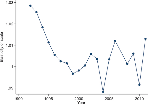
Figure 1 shows that the sample annual mean value for the elasticity of scale is close to one, denoting constant returns. The average elasticity of scale decreased slightly until 1999 (before Agenda 2000) and has stabilized around 1.0, but with increasing annual variability.

Figure 1. Dynamics of the elasticity of scale.

Figure 2 indicates that the patterns for neutral and overall technical change are quite similar, implying that for our sample of farms, technical progress is driven mainly by the neutral component. It is interesting to note that technical change was regressive (i.e. negative) until 2000 although it moved steadily upwards, slowly approaching 0% change. Since 2000, the results exhibit technical progress (i.e. a positive rate) and at the end of the period covered in this study, the rate was close to 1% per year.

Figure 2. Dynamics of technical change.

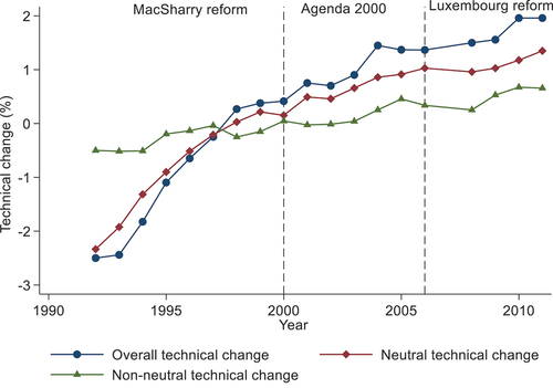
Regarding the pattern of non-neutral technical change, Table 2 indicates that the sign of the estimated coefficients of the variables ‘Labour × time’, ‘Capital × time’, and ‘Intermediate inputs × time’ are, respectively, negative, negative, and positive. This suggests that technical progress tends to diminish the use of labour and capital, and to increase the use of intermediate inputs. In other words, for our sample of French farms, technical progress is labour- and capital-saving, and is associated with an increase in the usage of intermediate inputs.

Technical efficiency results

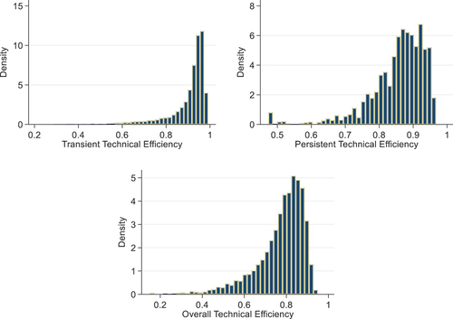
Table 3 shows that the average overall technical efficiency is 0.80. This implies that, on average, farms in our sample produce 20% below their potential output due to transient and persistent technical inefficiency. This result is consistent with other studies on technical efficiency in the agricultural sector (see Bravo-Ureta et al. 2007). The average persistent technical efficiency is 0.85, meaning that on average our sample of farms produce 15% below their potential output because of structural causes of technical inefficiency. It can also be seen from Table 3 that transient technical efficiency is 0.94 on average; hence, an average farm has little potential for production improvements (only 6%) in terms of transient factors, such as the capacity and skills of farmers to handle short-term deviations in the production process.

In the same vein, the results (Table 3) indicate that persistent technical efficiency is lower than transient on average. This suggests that the observed overall technical inefficiency is mainly due to factors that persist over time and that structural changes might offer good opportunities to improve productivity. From a policy point of view, these results highlight the importance of separating transient from persistent technical efficiency, given that they have different implications as to how to promote productivity growth.

The histograms in Figure 3 and the technical efficiency distributions in Table 3 show that, behind the mean technical efficiency, there is a large variation across farms. In addition, the summary statistics presented in Table 3 show that for 25% of the observations, persistent technical efficiency scores are below 0.82, and that 75% of the observations have scores for this type of efficiency below 0.91. The summary statistics by quartiles for technical change can be interpreted in a similar way.

Figure 3. Distribution of persistent, transient and overall technical efficiency scores in terms of histograms for the sample.

Explaining technical efficiency

The results concerning the inefficiency effects models are presented in the lower part of Table 2. Regarding the effect of the contextual drivers, a positive (negative) sign reveals a negative (positive) relationship with technical efficiency. The coefficient of total subsidies in the persistent inefficiency function is found to be positive and statistically significant at the 1% level, thus persistent technical efficiency decreases with an increase in public subsidies (per hectare) received by farms. A possible explanation for this finding is that public subsidies may encourage sluggish adjustments. This result is in line with Matthews (2013a, 1), who argues that ‘subsidies could slow down the rate at which resources are reallocated to more productive use in response to new technologies or market conditions’.

We also find that public subsidies are negatively associated with farm transient technical efficiency, suggesting that the extra income provided by such subsidies reduces the managerial efforts of farmers (Latruffe et al., 2017; Bojnec and Latruffe 2013; Martin and Page 1983; Sipiläinen, Kumbhakar, and Lien 2014; Skevas, Oude Lansink, and Stefanou 2012; Zhu and Oude Lansink 2010). Note that our findings suggest that public subsidies are negatively associated with both persistent and transient technical efficiency.

The efficiency results suggest that sole proprietorship is positively associated with both persistent and transient technical efficiency. A possible explanation for this result is the self-enforcing incentive of individual farmers to work more efficiently than workers in company farms (Mathijs and Vranken, 2000; Gorton and Davidova 20,004). Note, however, that there is no clear-cut conclusion in the literature on the effect of ownership type on farm performance (see Bakucs et al. 2010; Gorton and Davidova 2004).

Indebtedness, measured as the debt to assets ratio, is found to be positively associated with persistent technical inefficiency. While the effect of indebtedness on technical efficiency is ambiguous in the existing literature (see Davidova and Latruffe, 2007; Mugera and Nyambane, 2014), our findings could be linked to financial constraints for highly indebted farmers. This may slow down the adjustment of some production factors, leading to persistent technical inefficiency. In contrast, indebtedness is found to be positively associated with transient technical efficiency. This could be explained by the fact that indebted farmers tend to work more efficiently (in their daily management practices) to ensure their repayment capacity so as to avoid defaulting on debt obligations (Minviel and Sipiläinen, 2018).

Regarding the share of livestock output in total output, we find a positive association with both persistent and transient technical efficiency. This result could be explained by the fact that mixed crop-livestock farms oriented towards livestock production rely mainly on drivers (such as pastures, see Figure A1 in Appendix) associated with production practices, implying lower input usage for a given level of production than mixed systems oriented towards arable crops. As for the time-trend variable, no significant effect is found on transient technical efficiency. Note that the time-trend variable is not considered as a determinant of the persistent efficiency model, since persistent efficiency is by definition time-invariant.

Finally, Figure 4 depicts the dynamics of average annual persistent, transient and overall technical efficiency over the period covered by our data, which includes various CAP regimes. The figure shows that average persistent technical efficiency is quite stable over time while average transient and overall technical efficiency are more variable. Similar results can be found in Ayelign and Singh (2019). In addition, Figure 4 suggests that there are some changes in overall and transient technical efficiency with respect to the changes in the CAP regimes. According to the regime indicators, persistent technical efficiency was significantly higher in the first CAP regime period compared to the two latter ones. Note also that the persistent efficiency curve is slightly decreasing over the different CAP regimes. Similarly, Table 4 shows that the different CAP regimes (modelled by the average level of subsidies per farm during each CAP regime) are negatively associated with persistent efficiency.

Figure 4. Dynamics of average persistent, transient and overall technical efficiency for the sample.

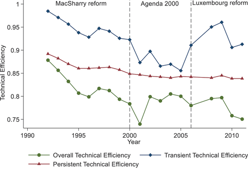
Table 4. Parameter estimates for the persistent inefficiency model with different specifications for the subsidy variable.

	Estimates	Standard errors
Estimates with mean of subsidies per farm for the CAP regimes in three different regimes
Subsidy per hectare over 1992–1999	0.290***	0.046
Subsidy per hectare over 2000–2005	0.167***	0.036
Subsidy per hectare over 2006–2011	0.119*	0.070
Sole proprietorship dummy	−0.125***	0.052
Share of livestock output	−0.026***	0.002
Debt to assets ratio	0.058***	0.005
Intercept	−0.965**	0.177
Estimates with mean of subsidies per farm for the CAP regimes in a unique variable
Subsidy per hectare	0.096***	0.034
Sole proprietorship dummy	−0.101**	0.051
Share of livestock output	−0.029**	0.014
Debt to assets ratio	0.087***	0.004
Intercept	−0.045***	0.018
Number of observations	6,685

The asterisks *, **, and *** indicate significance at the 10, 5 and 1% levels, respectively.

V. Concluding remarks

Several papers have analysed the link between agricultural policy changes and farm technical efficiency. Most of these papers are almost exclusively focused on overall technical efficiency measures, without distinguishing between transient and persistent inefficiencies. While transient inefficiency could change over time, even in the absence of changes in farm management practices, persistent inefficiency can only change through farm restructuring. In other words, persistent inefficiency is unlikely to vary unless major changes are made to drivers, such as public policies, that may affect farm management practices. Hence, distinguishing between transient and persistent inefficiency enables a consistent evaluation of whether changes in agricultural policies induce changes in farmers’ production decisions. This paper contributes to the literature by providing one of the first studies to analyse the subsidy-efficiency nexus while separating persistent from transient technical efficiency.

Our empirical analyses are conducted using unbalanced panel data of 6,685 observations from 810 French mixed (crop and livestock) farms over the period 1992–2011. The results indicate that public subsidies positively influence both transient and persistent technical inefficiency. The negative effects of subsidies on persistent efficiency suggest that public subsidies induce sluggish adjustments or restructuring in farms’ activities. The subsidy effect was negative for each CAP reform period, but persistent efficiency was significantly higher during the first reform.

Further analyses are needed on more recent data to compare findings under different CAP regimes. In addition, further research could be carried out to disentangle the subsidy effect depending on the type of subsidy. In particular, it would be interesting to understand whether agri-environmental subsidies play a similar role to decoupled subsidies. The former are meant to introduce a change in farming practices, while the latter are an income support instrument that can be received irrespective of farming practices. Furthermore, the work presented in this paper could be extended to account for different sources of spatial dependence among farmers (see Galli, 2023). This is highly relevant in the agricultural sector, because spatial proximity and unobserved spatial heterogeneity may be sources of productivity shock spillovers. For instance, unobserved spatial heterogeneity can arise from farmers emulating each other (Areal et al., 2012; Latruffe et al., 2013).

Disclosure statement

No potential conflict of interest was reported by the author(s).

Data Availability Statement

The stata codes used for the estimation are available from the corresponding author upon request.

Correction Statement

This article has been corrected with minor changes. These changes do not impact the academic content of the article.

Notes

¹ ${\upsilon }_{it}$ can also be assumed to be heteroscedastic.

² The z variables can also be modelled in the pre-truncated mean of $u_{it}$ (Badunenko and Kumbhakar, 2017).

³ This property does not always hold for other distributional assumptions, such as the normal-truncated-normal (Parmeter and Kumbhakar 2014).

Appendix

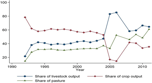
Figure A1. Sample’s averages of share of livestock output, share of crop output and share of pasture.

References

- Addo, F., and K. Salhofer. 2022. “Transient and Persistent Technical Efficiency and Its Determinants: The Case of Crop Farms in Austria.” Applied Economics 54 (25): 2916–2932. https://doi.org/10.1080/00036846.2021.2000580.
- Agasisti, T., and S. Gralka. 2019. “The Transient and Persistent Efficiency of Italian and German Universities: A Stochastic Frontier Analysis.” Applied Economics 51 (46): 5012–5030. https://doi.org/10.1080/00036846.2019.1606409.
- Aigner, D. J., C. A. K. Lovell, and P. Schmidt. 1977. “Formulation and Estimation of Stochastic Frontier Production Function Models.” Journal of Econometrics 6 (1): 21–37. https://doi.org/10.1016/0304-4076(77)90052-5.
- Amsler, C., A. Prokhorov, and P. Schmidt. 2016. “Endogeneity in Stochastic Frontier Models.” Journal of Econometrics 190 (2): 280–288. https://doi.org/10.1016/j.jeconom.2015.06.013.
- Anania, G., and M. R. Pupo D’Andrea. 2015. “The 2013 Reform of the Common Agricultural Policy.” In The Political Economy of the 2014-2020 Common Agricultural Policy: An Imperfect Storm, edited by J. Swinnen, 33–86. London: Rowman & Littlefield International, Ltd.
- Andor, M., and C. F. Parmeter. 2017. “Pseudolikelihood Estimation of the Stochastic Frontier Model.” Applied Economics 49 (55): 5651–5661. https://doi.org/10.1080/00036846.2017.1324611.
- Areal, F. J. K. Balcombe, and R. Tiffin. 2012. “Integrating Spatial Dependence into Stochastic Frontier Analysis.” The Australian Journal of Agricultural and Resource Economics 56: 521–541.
- Arellano, M. and O. Bover. 1995. “Another Look at the Instrumental Variables Estimation of Error-Components Models.” Journal of Econometrics 68: 29–51.
- Ayelign, Y., and L. Singh. 2019. “Short-Run and Long-Run Technical Efficiency Analysis: Application to Ethiopian Manufacturing Firms.” Seoul Journal of Economics 32 (4): 421–465.
- Badunenko, O. and S. C. Kumbhakar. 2017. “Economies of Scale, Technical Change and Persistent and Time-Varying Cost Efficiency in Indian Banking: Do Ownership, Regulation and Heterogeneity Matter?.” European Journal of Operational Research 260: 789–803.
- Bakucs, L., L. Latruffe, I. Ferto, and J. Fogarasi. 2010. “The Impact of EU Accession on farms’ Technical Efficiency in Hungary.” Post-Communist Economies 22 (2): 165–175. https://doi.org/10.1080/14631371003740639.
- Banker, R. D., A. Charnes, and W. W. Cooper. 1984. “Some Models for Estimating Technical and Scale Inefficiencies in Data Envelopment Analysis.” Management Science 30 (9): 1078–1092. https://doi.org/10.1287/mnsc.30.9.1078.
- Blundell, R. and S. Bond. 1998. “Initial Conditions and Moment Restrictions in Dynamic Panel Data Models.” Journal of Econometrics 87: 115–143.
- Bojnec, S., and L. Latruffe. 2009. “Determinants of Technical Efficiency of Slovenian Farms.” Post-Communist Economies 21 (1): 117–124. https://doi.org/10.1080/14631370802663737.
- Bojnec, S., and L. Latruffe. 2013. “Farm size, agricultural subsidies and farm performance in Slovenia.” Land Use Policy 32:207–217. https://doi.org/10.1016/j.landusepol.2012.09.016.
- Bokusheva, R., L. Čechura, and S. C. Kumbhakar. 2023. “Estimating Persistent and Transient Technical Efficiency and Their Determinants in the Presence of Heterogeneity and Endogeneity.” Journal of Agricultural Economics 74 (2): 450–472. https://doi.org/10.1111/1477-9552.12512.
- Bravo-Ureta, B., D. Solís, V. Moreira, J. Maripani, A. Thiam, and T. Rivas. 2007. “Technical Efficiency in Farming: A Meta-Regression Analysis.” Journal of Productivity Analysis 27 (1): 57–72. https://doi.org/10.1007/s11123-006-0025-3.
- Choi, O., S. E. Stefanou, and J. R. Stokes. 2006. “The Dynamics of Efficiency Improving Allocation.” Journal of Productivity Analysis 25 (1): 159–171. https://doi.org/10.1007/s11123-006-7138-6.
- Ciaian, P., and J. F. M. Swinnen. 2009. “Credit Market Imperfections and the Distribution of Policy Rents.” American Journal of Agricultural Economics 91 (4): 1124–1139. https://doi.org/10.1111/j.1467-8276.2009.01311.x.
- Coelli, T., A. Estache, S. Perelman, and L. Trujillo. 2003. A Primer on Efficiency Measurement for Utilities and Transport Regulators. Washington: World Bank Institute Development Studies.
- Colombi, R., S. C. Kumbhakar, G. Martini, and G. Vittadini. 2014. “Closed-Skew Normality in Stochastic Frontiers with Individual Effects and Long/short-Run Efficiency.” Journal of Productivity Analysis 42 (2): 123–136. https://doi.org/10.1007/s11123-014-0386-y.
- Davidova, S. and L. Latruffe. 2007. “Relationship Between Technical Efficiency and Financial Management for Czech Republic Farms.” Journal of Agricultural Economics 58: 269–288.
- European Commission. 2013. Overview of CAP Reform 2014-2020. Agricultural Policy Perspectives Brief, No 5.
- European Commission. (2017). The History of the Common Agricultural Policy. Internet. Accessed January 13, 2018. https://ec.europa.eu/agriculture/cap-overview/history_en.
- Farrell, M. J. 1957. “The Measurement of Productive Efficiency.” Journal of the Royal Statistical Society: Series A 120 (3): 253–281. https://doi.org/10.2307/2343100.
- Filippini, M., and W. Greene. 2016. “Persistent and transient productive inefficiency: a maximum simulated likelihood approach.” Journal of Productivity Analysis 45 (2): 187–196. https://doi.org/10.1007/s11123-015-0446-y.
- Galli, F.2023. “A Spatial Stochastic Frontier Model Including Both Frontier and Error-Based Spatial Cross-Sectional Dependence.” Spatial Economic Analysis 18 (2): 239–258.
- Gorton, M., and S. Davidova. 2004. “Farm Productivity and Efficiency in the CEE Applicant Countries: A Synthesis of Results.” Agricultural Economics 30 (1): 1–16. https://doi.org/10.1111/j.1574-0862.2004.tb00172.x.
- Greene, W. 2005a. “Fixed and Random Effects in Stochastic Frontier Models.” Journal of Productivity Analysis 23 (1): 7–32. https://doi.org/10.1007/s11123-004-8545-1.
- Greene, W. 2005b. “Reconsidering Heterogeneity in Panel Data Estimators of the Stochastic Frontier Model.” Journal of Econometrics 126 (2): 269–303. https://doi.org/10.1016/j.jeconom.2004.05.003.
- Greene, W.2007. Stochastic Frontier Models and Efficiency Analysis. LIMDEP 9.0 Reference Guide. Plainview, NY: Econometric Software Inc.
- Greer, A. 2013. “The Common Agricultural Policy and the EU Budget: Stasis or Change?” European Journal of Government and Economics 2 (2): 119–136. https://doi.org/10.17979/ejge.2013.2.2.4291.
- Johnson, R. 2007. “Farm Bill Proposals and Legislative Action in the 110th Congress.” Congressional Research Service Report. Washington, D.C.: Library of Congress, Congressional Research Service.
- Johnson, R., and J. Monke. 2014. “What is the Farm Bill?” Congressional Research Service Report, No RS22131.
- Kellerman, M. A. 2015. “Total Factor Productivity Decomposition and Unobserved Heterogeneity in Stochastic Frontier Models.” Agricultural and Resource Economics Review 44 (1): 124–148. https://doi.org/10.1017/S1068280500004664.
- Kumbhakar, S. C., and G. Lien. 2010. “Impact of Subsidies on Farm Productivity and Efficiency.” In The Economic Impact of Public Support to Agriculture: An International Perspective (Studies in Productivity and Efficiency), edited by V. E. Ball, R. Fanfani, and L. Gutierez, 109 124. New York, NY: Springer .
- Kumbhakar, S. C., G. Lien, and J. B. Hardaker. 2014. “Technical Efficiency in Competing Panel Data Models: A Study of Norwegian Grain Farming.” Journal of Productivity Analysis 41 (2): 321–337. https://doi.org/10.1007/s11123-012-0303-1.
- Kumbhakar, S. C., and C. F. Parmeter. 2019. “Implementing Generalized Panel Data Stochastic Frontier Estimators.” In Panel Data Econometrics: Theory, edited by M. Tsionas, 225–249. London: Academic Press, Elsevier.
- Kumbhakar, S. C., C. F. Parmeter, and V. Zelenyuk. 2020. “Stochastic Frontier Analysis: Foundations and Advances II”. In Handbook of Production Economics, In edited by S. Ray, R. Chambers, and S. C. Kumbhakar, Vol. 1. New York, NY: Springer .
- Kumbhakar, S. C., H. Wang, and A. P. Horncastle. 2015. A Practitioner’s Guide to Stochastic Frontier Analysis Using Stata. New York, NY: Cambridge University Press.
- Latruffe, L. 2010. Competitiveness, Productivity and Efficiency in the Agricultural and Agri-Food Sectors. OECD Food, Agriculture and Fisheries Papers, No. 30, OECD Publishing.
- Latruffe, L., B. E. Bravo-Ureta, A. Carpentier, Y. Desjeux, and V. H. Moreira. 2017. “Subsidies and Technical Efficiency in Agriculture: Evidence from European Dairy Farms.” American Journal of Agricultural Economics 99 (3): 783–799. https://doi.org/10.1093/ajae/aaw077.
- Latruffe, L. J. J. Minviel, and J. Salanié. 2013. The Role of Environmental and Land Transaction Regulations on Agricultural Land Price: The Example of Brittany. Centre for European Policy Studies (CEPS), Brussels. Factor Markets WP 14.
- Lence, S. H.2000. “Using Consumption and Asset Return Data to Estimate farmers’ Time Preferences and Risk Attitudes.” American Journal of Agricultural Econonomics 82 (4): 934–947.
- Lien, G., S. C. Kumbhakar, and H. Alem. 2018. “Endogeneity, Heterogeneity, and Determinants of Inefficiency in Norwegian Crop-Producing Farms.” International Journal of Production Economics 201:53–61. https://doi.org/10.1016/j.ijpe.2018.04.023.
- Mairesse, J. and B. H. Hall. 1996. Estimating the Productivity of Research and Development: An Exploration of GMM Methods Using Data on French and United States Manufacturing Firms. NBER Working Paper No. 5501.
- Manevska-Tasevska, G. H. Hansson, and K. Labajova. 2017. “Impact of Management Practices on Persistent and Residual Technical Efficiency–A Study of Swedish Pig Farming.” Managerial and Decision Economics 38 (6): 890–905.
- Manevska-Tasevska, G., H. Hansson, and K. Labajova. 2017. “Impact of Management Practices on Persistent and Residual Technical Efficiency: A Study of Swedish Pig Farming.” Managerial and Decision Economics 38 (6): 890–905. https://doi.org/10.1002/mde.2823.
- Martin, J. P., and J. M. Page Jr. 1983. “The Impact of Subsidies on X-Efficiency in LDC Industry: Theory and Empirical Test.” The Review of Economics and Statistics 64 (4): 608–617. https://doi.org/10.2307/1935929.
- Mathijs, E. and L. Vranken. 2000. Farm Restructuring and Efficiency in Transition: Evidence from Bulgaria and Hungary. Paper presented at the American Agricultural Economics Association Annual Meeting, Tampa, Florida, USA.
- Matthews, A. 2013a. “Greening Agricultural Payments in the Eu’s Common Agricultural Policy.” Bio-Based and Applied Economics 2 (1): 1–27.
- Matthews, A. 2013b. Impact of CAP Subsidies on Productivity. Internet. Accessed January 22, 2015. http://capreform.eu/impact-of-cap-subsidies-on-productivity/.
- Matthews, A. 2015. Two Steps Forward, One Step Back: Coupled Payments in the CAP. Internet. Accessed August 2, 2015. http://capreform.eu/two-steps-forward-one-step-backcoupled-payments-in-the-cap/.
- Minviel, J. J.2015. ”Public subsidies and farmers’ production decisions: A microeconomic analysis.” PhD diss., Humanities and Social Sciences. Université Européenne de Bretagne; AGROCAMPUS OUEST.
- Minviel, J. J., and L. Latruffe. 2017. “Effect of Public Subsidies on Farm Technical Efficiency: A Meta-Analysis of Empirical Results.” Applied Economics 49 (2): 213–226. https://doi.org/10.1080/00036846.2016.1194963.
- Minviel, J. J. and T. Sipiläinen. 2018. “Dynamic Stochastic Analysis of the Farm Subsidy Efficiency Link: Evidence from France.” Journal of Productivity Analysis 50: 41–54.
- Mugera, A. W. and G. G. Nyambane. 2014. “Impact of Debt Structure on Production Efficiency and Financial Performance of Broadacre Farms in Western Australia.” The Australian Journal of Agricultural and Resource Economics 59: 208–224.
- Mundlak, Y. 1961. “Empirical Production Function Free of Management Bias.” Journal of Farm Economics 43 (1): 44–56. https://doi.org/10.2307/1235460.
- Njuki, E., B. E. Bravo-Ureta, and V. E. Cabrera. 2020. “Climatic Effects and Total Factor Productivity: Econometric Evidence for Wisconsin Dairy Farms.” European Review of Agricultural Economics 47 (3): 1276–1301. https://doi.org/10.1093/erae/jbz046.
- Ogundari, K.2014. “The Paradigm of Agricultural Efficiency and Its Implication on Food Security in Africa: What Does Meta-Analysis Reveal?.” World Development 64: 690–702.
- Parmeter, C. F., and S. C. Kumbhakar. 2014. “Efficiency Analysis: A Primer on Recent Advances.” Foundations and Trends in Econometrics 7 (3–4): 191–385. https://doi.org/10.1561/0800000023.
- Pindyck, R. S. 1993. “A note on competitive investment under uncertainty.” The American Economic Review 83 (1): 273–277.
- Rizov, M., J. Pokrivcak, and P. Ciaian. 2013. “CAP Subsidies and Productivity of the EU Farms.” Journal of Agricultural Economics 64 (3): 537–557. https://doi.org/10.1111/1477-9552.12030.
- Serra, T., D. Zilberman, and J. M. Gil. 2008. “Farms’ Technical Inefficiencies in the Presence of Government Programs.” The Australian Journal of Agricultural and Resource Economics 52 (1): 57–76. https://doi.org/10.1111/j.1467-8489.2008.00412.x.
- Sipiläinen, T., S. C. Kumbhakar, and G. Lien. 2014. “Performance of Dairy Farms in Finland and Norway from 1991 to 2008.” European Review of Agricultural Economics 41 (1): 63–86. https://doi.org/10.1093/erae/jbt012.
- Sipiläinen, T., and A. Oude Lansink 2005. Learning in Organic Farming – an Application on Finnish Dairy Farms. Paper presented at the XIth Congress of the European Association of Agricultural Economists (EAAE), Copenhagen, Denmark.
- Skevas, T., A. Oude Lansink, and S. E. Stefanou. 2012. “Measuring Technical Efficiency of Pesticides Spillovers and Production Uncertainty: The Case of Dutch Arable Farms.” European Journal of Operational Research 223 (2): 550–559. https://doi.org/10.1016/j.ejor.2012.06.034.
- Stead, A. D., P. Wheat, and W. H. Greene. 2019. “Distributional Forms in Stochastic Frontier Analysis.” In Palgrave Handbook of Economic Performance Analysis, edited by T. ten Raa and W. H. Greene, 225–274. Cham, Switzerland: Palgrave Macmillan.
- Tsionas, E. G., and S. C. Kumbhakar. 2014. “Firm Heterogeneity, Persistent and Transient Technical Inefficiency: A Generalized True Random-Effects Model.” Journal of Applied Econometrics 29 (1): 110–132. https://doi.org/10.1002/jae.2300.
- Weil, P. 2002. “L’incertitude, le temps et la théorie de l’utilité.” Risques 49: 70–76.
- Zhu, X., G. Karagiannis, and A. Oude Lansink. 2011. “The Impact of Direct Income Transfers of CAP on Greek Olive farms’ Performance: Using a Non-Monotonic Inefficiency Effects Model.” Journal of Agricultural Economics 62 (3): 630–638. https://doi.org/10.1111/j.1477-9552.2011.00302.x.
- Zhu, X., and A. Oude Lansink. 2010. “Impact of CAP Subsidies on Technical Efficiency of Crop Farms in Germany, the Netherlands and Sweden.” Journal of Agricultural Economics 61 (3): 545–564. https://doi.org/10.1111/j.1477-9552.2010.00254.x.