Adstock revisited

ABSTRACT

The standard Adstock regression is problematic for at least two reasons. Statistical inference is cumbersome and there is a chance of a spurious relation between sales and advertising. This paper shows that reformulating the equation solves both problems, and the result is that a proper model for Adstock is an unrestricted Koyck model. Maximum Likelihood estimation gives the parameter estimates. An illustration to the illustrious monthly Lydia Pinkham data shows the merits of the method.

KEYWORDS:

• Sales and advertising
• adstock
• Koyck model
• spurious relations

JEL CLASSIFICATION:

• M31
• M37
• C32
• C52

I. Introduction and motivation

Broadbent (1979, 1984) introduced the concept of Adstock for understanding sales and advertising relationships, when the two variables are observed over time. It basically translates advertising into a cumulative advertising process, and next it proposes to regress sales on accumulated advertising. The concept has been and still is very popular in practice, see Ephron and McDonald (2002) and Dubé et al. (2005), as well as in the academic literature, see Cleeren et al (2008), Danaher et al, (2008), Donagoglu and Klapper (2006), Gijsenberg et al. (2012), and Steenkamp and Gielens (2003), Beltran-Royo et al (2016), Naimi et al. (2016), Havlena and Graham (2004), Aurier and Broz-Giroux (2014) and Yeh and Chang (2023), to mention just a few. Hence, even though the concept was proposed a long time ago, it is still use in applied economics studies.

The idea of the Adstock concept is the following. Consider advertising $A_t$ and sales $S_t$ for $\mathit{t}=1,2,3,..,\mathit{T}$, where the data can concern days or weeks or months. Assume for the moment that advertising is a stationary [I(0)] time series. Adstock is commonly defined as

(1) $\mathit{A}{A}_t=A_t+\mathit{\lambda A}{A}_{\mathit{t}-1}$(1)

where $0<\mathit{\lambda }<1$, which is a crucial assumption. Alternative versions of (1) can be found in Joy (2006), which typically involve replacing $A_t$ by $\mathit{f}\left(A_t\right)$, where $\mathit{f}\left(.\right)$ is a monotone function. For (1), the half-life $\mathit{\eta }$ is equal to $\frac{log0.5}{log\mathit{\lambda }}$, where log denotes the natural logarithm. Also, the notion of Adstock can easily include other marketing mix variables, making the forthcoming regression models more involved.

Next, in practice one usually resorts to the regression model

(2) $S_t=\mathit{\alpha }+\mathit{\beta A}{A}_t+{\epsilon }_t$(2)

where ${\epsilon }_t$ is often assumed to be a mean zero and uncorrelated error process with variance ${\sigma }_{\epsilon }^2$. Given a selected value of $\mathit{\lambda }$ in (1), one can create $\mathit{A}{A}_t$, and the parameters in (2) can be estimated using Ordinary Least Squares (OLS).

For at least two reasons, this methodology to examine the effects of advertising (or other marketing mix variables) is problematic. First, and as is often done in practice, one tends to maximize the fit of (2) by searching over values of $\mathit{\lambda }$. This favourably biases the statistical relevance of $\mathit{\beta }$. At the same time, it is an inconvenient method to estimate $\mathit{\lambda }$, as no standard errors around the estimator $\hat{\lambda }$ are obtained.

The second potential problem occurs in the case when there really is no effect of advertising on sales, and the true sales process is for example

$S_t=\mathit{\mu }+\mathit{\rho }{S}_{\mathit{t}-1}+{\nu }_t$

with $0<\mathit{\rho }<1$. The regression in (2) then gives spurious results, at a degree depending on the values of $\mathit{\lambda }$ and $\mathit{\rho }$. For example, if $\mathit{\lambda }=\mathit{\rho }=0.9$ and $\mathit{T}=100$, Table 1. A1 in Franses (2018) shows that in 50.5% of the simulated cases, one would find a 5% significant parameter $\mathit{\beta }$ in (2), in the actual case that sales and advertising are fully independent processes. Note that this parameter can be positive and can be negative. Theoretical results are presented in Granger, Hyung and Jeon (2001), see also Yule (1926).

Table 1. Searching for the optimal value of $\mathit{\lambda }$ using (1) with (2).

Estimates (standard error in parentheses)
$\mathit{\lambda }$	$\mathit{\beta }$	SE of $\mathit{\beta }$	$R^2$
0.1	0.197	(0.048)	0.228
0.2	0.201	(0.045)	0.262
0.3	0.203	(0.041)	0.295
0.4	0.203	(0.039)	0.324
0.5	0.200	(0.037)	0.346
0.6	0.196	(0.035)	0.358
0.7	0.187	(0.034)	0.349
0.8	0.147	(0.033)	0.253
0.9	0.012	(0.022)	0.006

The present paper presents a simple method to meet these two problems. This method will be given in the next section. After that, an illustration shows its empirical relevance. The last section concludes.

II. The solution

To solve the two problems at once, it is recommended to add an error term $u_t$ to (1), that is,

(3) $\mathit{A}{A}_t=A_t+\mathit{\lambda A}{A}_{\mathit{t}-1}+u_t$(3)

where $u_t$ is a temporally uncorrelated error term with mean 0 and variance ${\sigma }_u^2$. This added error term can capture measurement errors in $A_t$ and $\mathit{A}{A}_t$ in part due to uncertainty about the exact value of $\mathit{\lambda }$. This added error term opens the way to rewrite the model in (2) in a convenient way.

With $0<\mathit{\lambda }<1$, and using the familiar lag operator L, defined by $L^k{y}_t=y_{\mathit{t}-\mathit{k}}$, with $\mathit{k}\in \left\{\dots ,-2,-1,0,1,2,\dots .\right\},$ we can write (3) as

(4) $\mathit{A}{A}_t=\frac{A_t+u_t}{1-\mathit{\lambda L}}$(4)

Plugging (4) into (2) gives

(5) $S_t=\mathit{\alpha }+\mathit{\beta }\frac{A_t+u_t}{1-\mathit{\lambda L}}+{\epsilon }_t$(5)

Multiplying both sides of (5) with $1-\mathit{\lambda L}$, and re-arranging terms, gives

(6) $S_t=\left(1-\mathit{\lambda }\right)\mathit{\alpha }+\mathit{\lambda }{S}_{\mathit{t}-1}+\mathit{\beta }{A}_t+\mathit{\beta }{u}_t+{\epsilon }_t-\mathit{\lambda }{\epsilon }_{\mathit{t}-1}$(6)

As $\mathit{\beta }{u}_t+{\epsilon }_t-\mathit{\lambda }{\epsilon }_{\mathit{t}-1}$ is a process with only non-zero autocorrelation at the first lag, due to ${\epsilon }_t$ and ${\epsilon }_{\mathit{t}-1}$, we can write (6) as

(7) $S_t=\mathit{\mu }+\mathit{\lambda }{S}_{\mathit{t}-1}+\mathit{\beta }{A}_t+v_t+\mathit{\theta }{v}_{\mathit{t}-1}$(7)

where $\mathit{\theta }<0$, and where $v_t$ is an uncorrelated error term with mean 0 and variance ${\sigma }_v^2$. It is easy to see that $\mathit{\lambda }\ne \mathit{\theta }$. The parameters in this model (7) can be estimated using Maximum Likelihood or Iterative Least Squares. Given estimates of $\mathit{\lambda },\mathit{\beta },v_t\mathrm{and}\mathit{\theta }$, it is also possible to estimate ${\sigma }_u^2$ and ${\sigma }_{\epsilon }^2$.¹

The model in (7) is an unrestricted equivalent of the Koyck (1954) model, which in original format reads as

(8) $S_t=\mathit{\mu }+\mathit{\lambda }{S}_{\mathit{t}-1}+\mathit{\beta }{A}_t+v_t-\mathit{\lambda }{v}_{\mathit{t}-1}$(8)

as it is based on the infinite distributed lag model

(9) $S_t=\mathit{\alpha }+\mathit{\beta }{A}_t+\mathit{\beta \lambda }{A}_{\mathit{t}-1}+\mathit{\beta }{\lambda }^2{A}_{\mathit{t}-2}+\dots +{\epsilon }_t$(9)

Franses and van Oest (2007) show for (8) that statistical inference is complicated because $\mathit{\lambda }$ appears in front of $S_{\mathit{t}-1}$ and in front of $v_{\mathit{t}-1}$. This problem however disappears for (7). At the same time, (7) includes $S_{\mathit{t}-1}$, and the inclusion of this term prevents obtaining a potential spurious relationship between sales and advertising. Moreover, the estimation method gives a standard error for the estimated value of $\mathit{\lambda }$. In sum, simply adding an error term to the Adstock equation makes all problems to disappear.

When it is assumed that advertising $A_t$ is a process integrated of order 0, that is, it is a stationary process, and when $0<\mathit{\lambda }<1$, then $\mathit{A}{A}_t$ is also a stationary process. To make the regression model in (2), that is, $S_t=\mathit{\alpha }+\mathit{\beta A}{A}_t+{\epsilon }_t$ a balanced model, such that indeed ${\epsilon }_t$ is white noise, then sales $S_t$ is also a stationary process.

When advertising $A_t$ is a process integrated of order 1, that is, it is a non-stationary process, then with $0<\mathit{\lambda }<1$, it then follows that $\mathit{A}{A}_t$ is then also a non-stationary process. This implies that Equation (7)(7) $S_t=\mathit{\mu }+\mathit{\lambda }{S}_{\mathit{t}-1}+\mathit{\beta }{A}_t+v_t+\mathit{\theta }{v}_{\mathit{t}-1}$(7) is a cointegration relationship, and this cointegration relation is a stationary moving average process of order 1, see also Baghestani (1991).

The assumption that $0<\mathit{\lambda }<1$is crucial. When $A_t$ is I(0), and $\mathit{\lambda }=1$, then $\mathit{A}{A}_t$ is I(1), and for model (2) to hold, the cointegration relation is

$S_t=\mathit{\alpha }+\mathit{\beta A}{A}_t+{\epsilon }_t$

and hence $S_t$ is I(1). A consequence is that when $A_t$ is I(0) and $S_t$ is I(1), Equation (7)(7) $S_t=\mathit{\mu }+\mathit{\lambda }{S}_{\mathit{t}-1}+\mathit{\beta }{A}_t+v_t+\mathit{\theta }{v}_{\mathit{t}-1}$(7) does not hold. Additionally, when $A_t$ is I(1), and $\mathit{\lambda }=1$, then $\mathit{A}{A}_t$ is I(2), and for model (2) to hold, then $S_t$ is I(2). When $A_t$ is I(1) and $S_t$ is I(2), Equation (7)(7) $S_t=\mathit{\mu }+\mathit{\lambda }{S}_{\mathit{t}-1}+\mathit{\beta }{A}_t+v_t+\mathit{\theta }{v}_{\mathit{t}-1}$(7) again does not hold.

Finally, when advertising and sales simultaneously determine each other, Equation (7)(7) $S_t=\mathit{\mu }+\mathit{\lambda }{S}_{\mathit{t}-1}+\mathit{\beta }{A}_t+v_t+\mathit{\theta }{v}_{\mathit{t}-1}$(7) needs to be extended to a simultaneous equation system, where instruments can be lagged sales and advertising variables.

III. Illustration

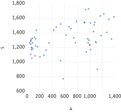
To illustrate the various aspects of the above discussion, consider the illustrious monthly Lydia Pinkham data in Figure 1, with a scatter in Figure 2. Table 1 shows the results of a rather rough grid search for finding the proper value of $\mathit{\lambda }$. Looking at the patterns in the standard errors for $\mathit{\beta }$ and the $R^2$ values, one would be inclined to believe that $\mathit{\lambda }$ is anywhere around 0.6. A more refined grid search could now follow.

Figure 1. Monthly Lydia Pinkham sales and advertising data, 1954.01–1958.12.

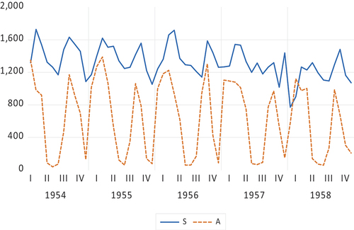
Figure 2. Monthly Lydia Pinkham sales against advertising data, 1954.01–1958.12.

However, if we resort to Maximum Likelihood estimation of (7) for 59 effective observations we obtain the parameter estimates (with standard errors in parentheses):

$\hat{\mu }=350.72\left(196.75\right)$

$\hat{\lambda }=0.635\left(0.155\right)$

$\hat{\beta }=0.208\left(0.046\right)$

$\hat{\theta }=-0.374\left(0.178\right)$

The $R^2=0.415$ and the Durbin Watson statistic is 1.954. We see that $\hat{\lambda }$ is indeed close to 0.6, but now we have an estimated standard error. The standard error for the associated $\mathit{\beta }$ is now 0.046, which is larger than those reported in Table 1, as expected.

Finally, using the calculation in footnote 1, we arrive at ${\hat{\sigma }}_{\mathit{\epsilon }}^2=14924.7$ and ${\hat{\sigma }}_{\mathit{u}}^2=101641$. The variance of the Adstock variable in (3) is 362,701 for $\mathit{\lambda }=0.635$, and hence the error term $u_t$ in (3) can indeed not be ignored.

IV. Conclusion

This paper has argued that the standard Adstock regression is problematic for at least two reasons. These problems can be alleviated by reformulating the equation (after adding an error term), which results in the fact that a proper model for Adstock is an unrestricted Koyck model. Maximum Likelihood estimates gives the parameter estimates. An illustration showed the merits of the method.

Acknowledgements

The author is grateful to the comments made by three anonymous referees.

Disclosure statement

No potential conflict of interest was reported by the author(s).

Notes

¹ The variance of the process $\mathit{\beta }{u}_t+{\epsilon }_t-\mathit{\lambda }{\epsilon }_{\mathit{t}-1}$ is ${\beta }^2{\sigma }_u^2+\left(1+{\lambda }^2\right){\sigma }_{\epsilon }^2$, where the latter equals the variance of $v_t+\mathit{\theta }{v}_{\mathit{t}-1}$, which is $\left(1+{\theta }^2\right){\sigma }_v^2$. The first order autocovariances for the two processes are $-\mathit{\lambda }{\sigma }_{\epsilon }^2$ and $\mathit{\theta }{\sigma }_v^2$, respectively. This gives two equations to solve for ${\sigma }_u^2$ and ${\sigma }_{\epsilon }^2$.

References

- Aurier, P., and A. Broz-Giroux. 2014. “Modeling Advertising Impact at Campaign Level: Empirical Generalizations Relative to Long-Term Advertising Profit Contribution and Its Antecedents.” Marketing Letters 25 (2): 193–206. https://doi.org/10.1007/s11002-013-9252-3.
- Baghestani, H. 1991. “Cointegration Analysis of the Advertising-Sales Relationship.” The Journal of Industrial Economics 39 (6): 671–682. https://doi.org/10.2307/2098669.
- Beltran-Royo, C., L. F. Escudero, and H. Zhang. 2016. “Multiperiod Multiproduct Advertising Budgeting: Stochastic Optimization Modeling.” Omega – International Journal of Management Science 59 (March 2016): 26–39. https://doi.org/10.1016/j.omega.2015.02.013.
- Broadbent, S. S. 1979. “One Way TV Advertisements Work.” Journal of the Market Research Society 21 (3): 139–166.
- Broadbent, S. S. 1984. “Modeling with Adstock.” Journal of the Market Research Society 26 (4): 295–312.
- Cleeren, K., M. G. Dekimpe, and K. Helsen. 2008. “Weathering Product-Harm Crises.” Journal of the Academy of Marketing Science 36 (2): 262–270. https://doi.org/10.1007/s11747-007-0022-8.
- Danaher, P. J., A. Bonfrer, and S. Dhar. 2008. “The Effect of Competitive Advertising Interference on Sales for Packaged Goods.” Journal of Marketing Research 45 (2): 211–225. https://doi.org/10.1509/jmkr.45.2.211.
- Donagoglu, T., and D. Klapper. 2006. “Goodwill and Dynamic Advertising Strategies.” Quantitative Marketing and Economics 4 (1): 5–29. https://doi.org/10.1007/s11129-006-6558-y.
- Dubé, J. P., G. J. Hitsch, and P. Machanda. 2005. “An Empirical Model of Advertising Dynamics.” Quantitative Marketing and Economics 3 (2): 107–144. https://doi.org/10.1007/s11129-005-0334-2.
- Ephron, E., and C. McDonald. 2002. “Media Scheduling and Carry-Over Effects: Is Adstock a Useful TV Planning Tool?” Journal of Advertising Research 42 (4): 66–71. https://doi.org/10.2501/JAR-42-4-66-70.
- Franses, P. H., and R. van Oest. 2007. “On the Econometrics of the Geometric Lag Model.” Economics Letters 95 (2): 291–296. https://doi.org/10.1016/j.econlet.2006.10.023.
- Franses, P. H. 2018. Enjoyable Econometrics. Cambridge UK: Cambridge University Press.
- Gijsenberg, M. J., H. J. van Heerde, M. G. Dekimpe, and V. R. Nijs. 2012. Understanding the role of adstock in advertising decisions. Unpublished manusscript.
- Granger, C. W. J., N. Hyung, and Y. Jeon. 2001. “Spurious Regressions with Stationary Series.” Applied Economics 33 (7): 899–904. https://doi.org/10.1080/00036840121734.
- Havlena, W., and J. Graham. 2004. “Decay Effects in Online Advertising: Quantifying the Impact of Time Since Last Exposure on Branding Effectiveness.” Journal of Advertising Research 44 (4): 327–332. https://doi.org/10.1017/S0021849904040401.
- Joy, J. 2006. “Understanding advertising adstock transformations, MPRA paper 7683.” SSRN Electronic Journal. https://doi.org/10.2139/ssrn.924128.
- Koyck, L. M. 1954. Distributed Lags and Investment Analysis. Amsterdam: North Holland.
- Naimi, T. S., C. S. Ross, M. B. Siegel, W. DeJong, and H. Jernigan. 2016. “Jernigan 92016), Amount of Televised Alcohol Advertising Exposure and the Quantity of Alcohol Consumed by Youth.” Journal of Studies on Alcohol and Drugs 77 (5): 723–729. https://doi.org/10.15288/jsad.2016.77.723.
- Steenkamp, J. B. E. M., and K. Gielens. 2003. “Consumer and Market Drivers of the Trial Probability of New Consumer Packaged Goods.” Journal of Consumer Research 30 (3): 368–384. https://doi.org/10.1086/378615.
- Yeh, L. T., and D.-S. Chang. 2023. “Measuring the Lagged Effects of Advertising Goodwill on Dynamic Promotional Efficiency in the Automobile Industry.” Journal of the Operational Research Society 74 (10): 2094–2108. in print. https://doi.org/10.1080/01605682.2022.2128910.
- Yule, G. 1926. “Why Do We Sometimes Get Nonsense-Correlations Between Time-Series?--A Study in Sampling and the Nature of Time-Series.” Journal of the Royal Statistical Society 89 (1): 1–64. https://doi.org/10.2307/2341482.