The reverse mortgage market in New Zealand: key drivers of loan determination

ABSTRACT

This paper examines the drivers of loan principals in the reverse mortgage and equity release market in New Zealand using a hedonic price model (HPM) approach. Our analysis using reverse mortgages data between 2004–2021, sourced from one major reverse mortgage bank, provides four key findings. First, the term of payment for repaid reverse mortgages is positively associated with loan principals, implying that longer repayment terms allow applicants who were able to repay mortgages to borrow more. Second, there is partial evidence to suggest the presence of a positive linear impact of the value of the current property on its loan principal, in line with previous house price modelling studies. Third, older applicants (age 75+) borrow less than younger applicants, which may be due to their repaying ability. Fourth, we confirm a positive effect of interest rates on reverse mortgage amounts but reject the positive association between wider loan-to-value policy restrictions and equity release lending amounts. The results broadly highlight that the house price is more relevant than any individual characteristic of a property in determining loan principals, and that all drivers are relevant in the early stage of the development of the reverse mortgages market in New Zealand.

KEYWORDS:

• Reverse mortgages
• equity release
• ageing population
• housing finance

JEL CLASSIFICATION:

• G51
• L85
• R30

I. Introduction

According to the World Health Organization (2022), by 2030, one in six people will be aged 60 or over, and the number of people in this age bracket will double to 2.1 billion by 2050. In certain countries, the situation is more acute: for example, one in 10 people in Japan are now aged 80 or over (Robine 2021). This demographic shift is attributed to declining fertility rates and increased longevity. However, the extended lifespan often comes with health challenges, placing additional burdens on healthcare systems (World Health Organization 2022). In many advanced societies, the senior population cohorts benefit from high levels of home ownership and are often mortgage-free by the time they retire.

One financial option for those with housing assets, and wishing to release capital, is to take out an equity release, or reverse mortgage. Reverse mortgages allow people close to, or in, retirement to borrow against the value of their home. The interest is compounded during the life of the loan. Repayment of capital and interest can be at the point of death, moving into care, or as an early voluntary repayment. In essence, a reverse mortgage is a bank loan, secured on the value of the property. The amount borrowed is affected by the applicant’s age and the market value of the home. Opinions on the reverse mortgage market cover both positive aspects, such as enabling greater access to cash when circumstances change, and negative aspects, such as a diminished estate and a burden of debt (Weber and Chang 2006).

This study focuses on reverse mortgage lending in New Zealand with an ageing population profile but a high proportion of asset wealth in property (Squires and Webber 2019). Lissington (2018) estimated that fewer than 47% of retirees in New Zealand were enjoying a lifestyle in retirement similar to pre-retirement levels. Therefore, many retirees might be looking for additional sources of finance to release cash to fund health care and/or activities in retirement.

The reverse mortgage market in New Zealand has grown, with over NZ$710 m in issue and outstanding as of January 2023 (Hatton 2023), but is provided by only a handful of non-mainstream commercial banks. As of 30 June 2021, when the reverse mortgage portfolio was NZD$602 m, the average loan size was NZD$109,417 (PWC 2021). Such ‘early stage’ development of the reverse mortgage market in New Zealand, therefore, is worth examining to understand its characteristics and determinants, which could help further to develop the market.

Many previous real-estate studies have used the hedonic price model (HPM) to examine the impacts of the property’s and borrower’s characteristics on its price (e.g. Chin and Chau 2003; Meese and Wallace 1991). In this study, we examine the reverse mortgage principal loan value and its determinants in New Zealand, with a particular focus on whether house prices are more important than borrowers’ characteristics.

The paper is structured as follows. In the next section, we review the literature surrounding reverse mortgages, explore its association with housing asset-based welfare, and consider the growth of reverse mortgages more broadly. Section II presents the methodology and data. Section III reports the results, followed by a discussion of the key findings in Section IV. Finally, in Section 6, we conclude with implications for policy and practice.

II. Literature

Market growth

Homeownership has grown with government housing policies and developments in mortgage markets. The last 50 years have witnessed the financialization of the asset class, with homeowners enjoying high levels of capital gain through high house price inflation caused by housing shortage, low interest rates, and higher borrowing levels. The life-cycle theory of consumption and savings, developed by Modigliani and Brumberg (1954) and Ando and Modigliani (1963), posits that individuals plan their consumption over their life-cycle, accumulating funds when they are earning, paying off their mortgage and putting aside money into pension schemes and savings accounts, and then spending their accumulated wealth when they retire.

In the United States, the expansion of the mortgage market using reverse mortgages has been significant (Chatterjee 2016; Merrill, Finkel, and Kutty 1994), with suggestions that higher house prices will lead to more reverse mortgages (Shan 2011).

An ageing population

Reverse mortgages are influenced by an ageing population with fewer people in the labour force and more people spending (rather than investing) their savings, which can hinder economic growth (Marešová, Mohelská, and Kuča 2015). The need for social care support further complicates the situation, raising issues around intergenerational resource distribution. Many older individuals, therefore, prefer to stay at home and ‘age in place’ (Tinker 2002), which often requires structural adaptations to be made to homes to cater for the occupant’s physical and mental decline. Despite replacement fertility and younger net migration, New Zealand experiences ageing effects at a sub-national level (Jackson and Cameron 2018)

Retirement villages have been expanded to meet the demands of the ageing population, offering care packages for partially independent living (Grant 2006). Utilizing housing equity in financial planning provides psychological and financial benefits for those who wish to remain in their homes (Cutler 2003). Reverse mortgages offer a means of retaining one’s home while accessing financial security in later life (Costa-Font, Gil, and Mascarilla 2010; Leviton 2001).

Governments respond to the ageing population by raising the pension age and adjusting eligibility criteria: riots erupted in France when the retirement age was increased from 62 to 64 (B.B.C. 2023) and questions were raised over affordability in the UK when the Centre for Social Justice (2019) suggested raising the state pension age in the UK to 75 by 2035. Means-testing the state pension based on retirees’ total assets is a potential future consideration, with possible opposition from influential retiree voters.

The current pension age of 65 in New Zealand is being phased in to rise to 67 by 2040 (New Zealand Government 2017). The state pension, known as ‘NZ Super’, is constrained by political and economic barriers. This creates a socio-economic welfare concern as up to 40% of those over 65 rely solely on the NZ Super and 20% have ‘only a little more’ Retirement Commission (2023). This poses challenges in terms of self-sufficiency and covering housing expenses in retirement.

Housing asset-based welfare (HABW)

The ageing population has led governments to consider asset-based welfare as a means of shifting responsibility for services from the state to individuals (Doling and Ronald 2010). In countries like the UK, this often involves using housing assets, hence the term ‘housing asset-based welfare’ (HABW) (Fox O’Mahony and Overton 2015). Homeowners may need to use their assets to fund their own welfare, such as private healthcare, when the state system is strained (Montgomerie and Büdenbender 2015).

Authors like Kemeny (1981), Castles (1998), De Decker and Dewilde (2010), Lennartz and Ronald (2017), and Sendi et al. (2019) have discussed HABW as a supplement or replacement for the state pension. Toussaint and Elsinga (2009), however, raised concerns about HABW. Firstly, connecting welfare levels with house prices poses risks due to price volatility. Housing and welfare demand often diverges, as recessions may decrease house prices while increasing welfare demands. Secondly, HABW policies must be inclusive, but lower-income groups struggle to enter homeownership, exacerbating social inequalities. Lastly, equity-release products rely on house price inflation, which can lead to negative equity in declining markets. The affordability of homeownership and equity-release products is influenced by macroeconomic interest rates (Squires et al. 2022).

The functioning of the market

Equity release mortgages and their funding sources vary across countries. In the UK, insurance companies are the main funders, but the attractiveness of the product has declined due to falling annuity rates and complications with Solvency II (Sharma, French, and McKillop 2022b). In the US, securitization is the primary funding source, while Australia and Sweden rely on a mix of securitization and bank lending, whereas funding in Spain is from a combination of bank debt and insurance, and in Canada bank debt and whole portfolio sales (EPARG 2021). New Zealand’s funding mainly comes from banks, specifically SBS Bank and Heartland Bank (Heartland Group 2022; SBS Bank 2023).

Equity release mortgages are not considered suitable for long-term care funding, as they were not designed for that purpose. There is reluctance among borrowers to use accumulated housing equity for care needs, reflecting resistance to the concept of housing asset-based welfare. The spatial concentration of equity release mortgage supply is observed in a few UK regions due to the risk associated with lending in areas with low house price growth (Hosty et al. 2008; Sharma, French, and McKillop 2022a). In the US, reverse mortgages are used as a hedge against potential future house price declines, with higher demand from lower-income and older age groups (Haurin, Moulton, and Shi 2018; Moulton et al. 2017). Also in the US, there are demographic patterns where the demand for reverse mortgages has experienced a higher rate of application from lower-income and older age groups (Nakajima and Telyukova 2017).

Several authors (Nakajima and Telyukova 2013; Pu, Fan, and Deng 2014; Sharma, French, and McKillop 2022a, 2022b) reflect on the additional cost of the No Negative Equity Guarantee (NNEG), manifested in upfront fees and higher interest rates, and its dampening effect on the LTVs. Upfront fees in the South Korean market were found to be insufficient to cover the cost of non-recourse protection (Kim and Li 2017). Consequently, the value of NNEG for regulatory requirements has been estimated, and risk models have been developed to assess house price, mortality, and interest rate risks in equity-release mortgage portfolios (Fuente, Navarro, and Serna 2021, 2023).

In Australia, increasing LTVs and reducing insurance premiums or ongoing fees are recommended to grow the market, but the initial age of borrowers significantly impacts profitability (Alai et al. 2014). Concerns over financial literacy and reluctance to mortgage properties were observed among Australian retirees (De Silva et al. 2016). Studies in the UK and South Africa noted some reluctance to adopt equity-release mortgages, but attitudes towards debt were changing, with formal property rights playing an important role (Luiz and Stobie 2010).

III. Methodology and data

Data

Data were collected from a single major reverse mortgage bank provider in New Zealand, Heartland Bank.¹ The bank has been offering a reverse mortgage service to New Zealanders since 2004 and, as of 30 September 2022, Heartland has maintained its position as the largest active provider with a market share of 35.9% and ‘has helped more than 20,000 New Zealanders to live a more comfortable retirement under a total of NZD$721 million of receivables’ (Heartland Group 2022). In this research, we use every successful, and now closed, reverse mortgage application as an observation, resulting in a cross-sectional sample of 10,584 approved applications between June 2004 and June 2021.² It is, therefore, the richest data on New Zealand reverse mortgage market.³

Table 1 reports the descriptive statistics. The loan principal (RM, the actual loan that a mortgagee gets from the bank) of an average borrower was NZD$49,267.23, although it can range from as small as NZD$2,500 to as much as NZD$980,000. Consequently, the average value of RM is less than seven per cent of the value of the mortgaged property (which is NZ$718,526.80, see Table 1) and much lower than the permitted value accepted by the banks (which is 35.34%, see Table 1). This striking difference between actual (seven per cent) and permissible (35.34%) LTVs, suggests that New Zealand mortgagees either had different perceptions as to the function of the product, or had different requirements, or had concerns about it that resulted in low actual LTVs. In the first case, the market may be conceived as providing an alternative to bank loans; in the second, mortgagees may have limited capital requirements so require only low LTVs; and, in the third, the product may be regarded with caution because of perceptions of risk and cost. We have no information that would allow us to distinguish among these possibilities, except to suggest that lower capital requirements seem unlikely. This finding is interesting as, in comparison, Australian borrowers tend to apply for the maximum limit that had been permitted by their lenders (Australian Securities and Investments Commission 2018).

Table 1. Descriptive statistics of the variables of interest.

Variable	Unit	Mean	Standard deviation	Min	Max
Dependent variable
RM	NZ$	49,267.23	47,365.26	2,500.00	980,000.00
Independent variables X (Bank assessment)
term	year	5.70	4.63	0.00	17.23
permit	per cent	35.34	8.02	13.00	66.00
investment	dummy	0.00	0.04	0.00	1.00
Independent variables Y (Property characteristics)
value	NZ$	718,526.80	489,981.10	76,773.00	10,736,415.00
apartment	dummy	0.01	0.12	0.00	1.00
bungalow	dummy	0.45	0.50	0.00	1.00
flat	dummy	0.09	0.29	0.00	1.00
house	dummy	0.31	0.46	0.00	1.00
lifestyle	dummy	0.01	0.10	0.00	1.00
terraced	dummy	0.00	0.04	0.00	1.00
other	dummy	0.13	0.33	0.00	1.00
Independent variables Z (Borrower characteristics)
age_at_start	Years-old	71.64	6.44	55.00	98.00
male	dummy	0.18	0.38	0.00	1.00
female	dummy	0.42	0.49	0.00	1.00
joint	dummy	0.40	0.49	0.00	1.00
exit_deceased	dummy	0.00	0.05	0.00	1.00
exit_move2care	dummy	0.05	0.22	0.00	1.00
exit_voluntary	dummy	0.95	0.22	0.00	1.00
Control variables R
gdppc	NZ$	47,977.46	12,327.89	23,923.00	81,147.00
rates	per cent	7.32	2.09	4.47	10.72
LTVrestrict	dummy	0.48	0.50	0.00	1.00
Number of Observations: 10584

RM, loan principal; term, duration of the loan – all loans in the analyses have been completed/closed; permit, maximum proportion of RM allowed by the bank regarding the value of the property; investment, if the property is an investment; value, the value of the property accessed by the bank at time of application; apartment, bungalow, flat, house, lifestyle, terraced, and other represent the type of the property; age_at_start, age of the borrower at time of approval; male, female, and joint represent the gender of the borrowers; exit_deceased, exit_move2care, and exit_voluntary represent how borrowers exited the mortgages; gdppc, nominal GDP per capita; rates, 1-year floating mortgage lending rates; LTVrestrict, if the mortgages were approved after the Loan-To-Value restriction in October 2013.

Mortgages are repaid either when the borrowers pass away (i.e. exit_deceased) or when they sell their houses (i.e. exit_move2care and exit_voluntary). An important feature of the New Zealand Reverse Mortgage market is that the majority (95% in this sample) of loans are repaid voluntarily prior to death, meaning that many Reverse Mortgage loans are used as a substitute for short-term lending. This suggests that, in a booming real estate market such as New Zealand (see Figure 1), most of the mortgagees may have decided to sell their houses to enjoy the benefits of such a market.⁴

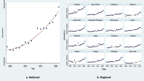
Figure 1. Valuation of house at application of reverse mortgage by year.

Source: Authors.

An initial look at the data shows that an applicant for a reverse mortgage is, on average, a 72-year-old (single) female. There are also many joint owners, accounting for about 40% of our sample (i.e. joint = 0.4). The housing stock is likely to be a bungalow or house valued at around NZ$718,000. As already noted, most of the applicants exit their mortgages voluntarily (i.e. exit_voluntary = 0.95) at 5.7 years (i.e. term = 5.7).

Methods

Our baseline model has a form of

(1) $\mathit{RM}=\mathit{\alpha }+{\beta }_i{X}_i+{\gamma }_j{Y}_j+{\delta }_k{Z}_k+{\delta }_r{R}_r+\mathit{\epsilon }$(1)

where RM is the loan principal (in natural logarithm) of an approved home-loan application⁵; X is a vector of variables that represent the assessment of the bank regarding the application (such as loan term or permitted value for the loan-to-value (LTV) ratio); Y is a vector of variables that describe the characteristics of the property involved (such as house value or house type); Z is a vector representing the characteristics of the applicant (such as gender or age); R is a vector of control variables (such as regional income and regional fixed effects variables); and $\mathit{\epsilon }$ is the error component. In this sense, in terms of the variables X and Z, Equation (1)(1) $\mathit{RM}=\mathit{\alpha }+{\beta }_i{X}_i+{\gamma }_j{Y}_j+{\delta }_k{Z}_k+{\delta }_r{R}_r+\mathit{\epsilon }$(1) follows the bank risk and credit-scoring theories (Carter et al. 2007; Laeven and Levine 2009; Laufer and Paciorek 2022). For variable Y, it is the hedonic price model (HPM) (e.g. Malpezzi 2003; Meese and Wallace 1991; Sirmans, Macpherson, and Zietz 2005) being examined.

The X variables, representing the bank’s assessment, may be derived from the characteristics of the applicants and the relevant property. However, the bank’s procedure is not transparent. Therefore, we test for multicollinearity among the X, Y, and Z variables in Section 4.3 below. Particularly, we first look at the LTV (i.e. permit) that an applicant is allowed to borrow. This represents the maximum LTV and thus, the maximum reverse mortgage principal that the bank allows a certain applicant to borrow. It mostly depends on the assessment of the bank regarding the risks associated with the loan. Therefore, it is not only the risk-aversion attitude of the bank that can influence permit (Boyd and De Nicoló 2005; Laeven and Levine 2009) but also the profile of the applicant (e.g. income, asset, gender or borrowing purpose) (Carter et al. 2007; Fuente, Navarro, and Serna 2021; Laufer and Paciorek 2022). In this sense, permit could account for other factors that may be missing from our analysis, as they should have been efficiently assessed by the bank, and for which we do not have data. A higher permit indicates a lower ‘price’ of the reverse mortgage since it requires less (initial) deposits (Ebrahim, Shackleton, and Wojakowski 2011), allows higher leverages, and less demanding underwriting standards, and thus develops a mortgage-price spiral (Arsenault, Clayton, and Peng 2013).

Given the role of permit, the two additional X variables that are also being examined include the calculated term of the reverse mortgage (i.e. term) and the type of the current mortgage (i.e. investment). It is noted that there is no pre-fixed due date for a reverse mortgage; the mortgage is due only when the borrowers move out or die (Nakajima and Telyukova 2017). In this sense, if the value of term is greater than zero, it indicates that the reverse mortgage has been paid, so normally a lower reverse mortgage would be accompanied by a shorter repayment term (Rasmussen, Megbolugbe, and Morgan 1997). Besides, if the current mortgage can generate some income for the borrowers (i.e. in the form of an investment property), a higher RM is expected. We accordingly propose our first hypothesis as follows:

H1:

There is a positive relationship between the X variables (i.e. permit, term, and investment) and RM.

The Y variables of the characteristics of the current property affect a property’s value, which affects the amount of the reverse mortgage. However, we also expect that different types of the property have different impacts on RM, following the hedonic price model (McCord et al. 2018; Ngo et al. 2023). For instance, Nicholas et al. (2001) argued that the property type reflects its architectural style (e.g. brick or cement, vintage or modern) which can affect its value, whilst Rehm and Filippova (2008) found that, in Auckland, a bungalow was worth $85,000 less than the normal (modern) house. Since we are unable to analyse the detailed house characteristics (e.g. size, school zone, or distance to shopping centres) due to data limitation, we examine whether property type plays any role in the borrowing decision of the mortgagees. While the detailed characteristics may be captured in value, the RM is still influenced by the borrowers’ own evaluation of the property, and their expectations of the repayment ability depending on the type of the current mortgage (Kelly, McCann, and O’Toole 2018; Park and Bang 2014). Therefore, if an applicant believes that their property has high value (e.g. being a house or apartment), they will have more incentive to apply for (a higher) loan principal. Consequently, our hypothesis regarding the Y variables is as follows.

H2:

There is a positive relationship between the value of the current property (i.e. value) and RM, but its characteristics (e.g. house, flat, and lifestyle) have different impacts on RM.

Regarding Z variables, the bank risk and credit-scoring theories (Demyanyk and Van Hemert 2009; LaCour-Little 1999) suggest that borrower characteristics are important factors that influence the mortgage decisions of both borrowers and lenders. For instance, Goldsmith-Pinkham and Shue (2023) found a gap in housing returns between male and female investors in the United States, suggesting that their earnings and thus, mortgage repayment abilities, are different. Consequently, there should be differences in the decision to borrow across male, female, and joint applicants. Using Indian microdata, Saha et al. (2022) argued that housing loan default, which is important to the lenders, is associated with the nature of employment, gender, socio-religious, and age of the borrowers. Brown et al. (2019) found that the risk tolerance reduces for higher age groups (i.e. 60–64, 65–69, and 70+). Since reverse mortgages are only available to people aged over 55 (Heartland Bank 2023), we are more interested in the gender of the applicants, their age (at the time of applying), and more importantly, how the reverse mortgage was repaid (e.g. exit via repayment or through death). Our third hypothesis is, therefore:

H3:

The impacts of the Z variables of borrower characteristics regarding their gender (i.e. male, female, and joint applicants), their age (i.e. age_at_start), and their exit strategies (i.e. through death, move to care or voluntarily) have different impacts on RM.

We further control for the intrinsic characteristics across the reverse mortgages. Firstly, as pointed out by Ngo et al. (2023), house prices and values vary across regions in New Zealand, we also include the regional dummy variables (e.g. Auckland and Wellington) in the R variables to control for such fixed effects. Secondly, the demand for reverse mortgages is proxied via the regional GDP per capita. Thirdly, following Rasmussen et al. (1997) and Nakajima and Telyukova (2017), we argue that people living in high-income regions are less likely to have to rely on reverse mortgages, i.e. a negative association between gdppc and RM. Fourthly, we also control for the changes in the 1-year floating mortgage lending rates (i.e. rates), which can also capture the macroprudential policy regarding the reverse mortgage market (Fuente, Navarro, and Serna 2023; Funke, Kirkby, and Mihaylovski 2018; Hargreaves 2016).

It is argued that rates also reflects inflation, the latter could affect the consumption level of the applicants and may require them to adjust their RM accordingly (Pfau 2016; Tsai, Wang, and Chang 2023). Among the macroprudential policies, the Reserve Bank of New Zealand (RBNZ) had notably decided to limit its financial institutions to have their high LTV (>80%) home loans to be at most 10% share of their total new loans in October 2013 (Hargreaves 2016; Reserve Bank of New Zealand 2023). Such ‘speed limit’ restrictions helped ease the ‘bubbly episodes’ in the national housing market (Greenaway-McGrevy and Phillips 2016). We, therefore, also include a dummy variable LTVrestrict (which has the value of unity for the years after 2013 and zero otherwise) in the set of R control variables to account for that policy. Consequently, our fourth hypothesis can be stated as follows:

H4:

The control variables R (i.e. gdppc, rates, and LTVrestrict) have different impacts on RM, in which the first two variables positively increase RM while the last one has a negative effect on RM.

IV. Empirical results

House valuations, loan principals, and LTV’s trend

The patterns or geometric growth in most markets throughout the study period are clear in Figure 1. The national average valuation at the time of the reverse mortgage application rose from NZD$200,000 in 2004 to NZD$800,000 in 2021 (Figure 1(a)). It is also clear that house price valuations have risen at different rates in different regions, although the mechanism for such increases needs to be examined in detail (see the following Section). For instance, Auckland had the steepest rise while the more sparsely populated West Coast region had the flattest valuation rise (Figure 1(b)).

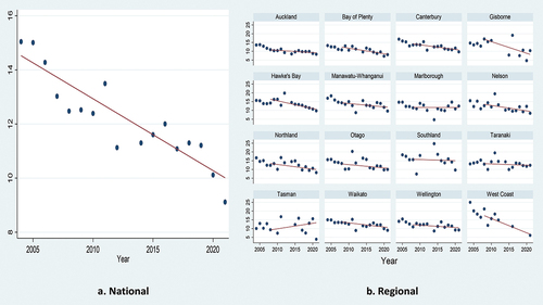
Figure 2 shows that the loan principals taken out as a reverse mortgage follow a national trajectory of decline towards the GFC of 2007–08, followed by a continual increase from NZD$37,000 in 2008 to NZD$65,000 in 2021 (Figure 2(a)). We also observe the same common trend across all regions during the same periods (Figure 2(b)). Simultaneously, Figure 3(a) shows a decline of the LTV ratios over the examined period (2004–21), although the LTV trend varies across regions: the West Coast region finds a steep decline in LTV, whilst Auckland experienced a more gradual decline, and the Tasman region has an increase but with more variance (Figure 3(b)). Such variance was largely due to fewer mortgages taken out in the less populous Tasman region, which has a wide range of property values in its sub-market. Overall, the variances presented in Figures 1(b), 2 (b), and 3(b) reflect that the sample of houses varies from year to year, and the changes in values may reflect more than general market movements, but also the composition (such as size and type) of the applications.

Figure 2. Loan principals at application of reverse mortgage by year.

Source: Authors.

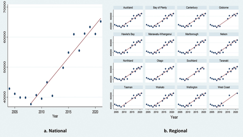
Figure 3. LTV at application of reverse mortgage by year.

Source: Authors.

Results and discussions

We start our estimation of Equation (1)(1) $\mathit{RM}=\mathit{\alpha }+{\beta }_i{X}_i+{\gamma }_j{Y}_j+{\delta }_k{Z}_k+{\delta }_r{R}_r+\mathit{\epsilon }$(1) with Model 1 using all variables as in Table 1. To further test for the non-linear effects of permit and value, we first include the squares of only permit (i.e. permit²) into Model 2, the squares of only value (i.e. value²) into Model 3, and both permit² and value² into Model 4 of the analysis. Monetary variables (e.g. value and gdppc) have been deflated before estimation. Estimated results from those models using a heteroskedasticity-consistent covariance matrix estimator type 3 (HC3) method are reported in Table 2, where it can be observed that the results for the X, Y, Z, and R variables are generally consistent across the models, showing that the bank’s assessment, house value, age over 75, interest rates and government policy are significant factors in the New Zealand reverse mortgage market. It is also noted that, although the R² statistics of our models are not high, this is common for regressions with thousands of observations (Lin and Wiegand 2023; Pérez-Rave, Correa-Morales, and González-Echavarría 2019; Rafei, Flannagan, and Elliott 2020).

Table 2. Estimation results from OLS regressions.

Dependent variable: RM	Model 1	Model 2	Model 3	Model 4
X variables (Bank assessment)
term	0.004**	0.004**	0.004**	0.004**
permit	0.531***	-0.040	0.532 ***	-0.054
permit^2		0.086		0.088
investment	0.215	0.213	0.216	0.215
Y variables (Property characteristics)
value	0.515***	0.516***	0.554***	0.566***
value^2			-0.003	-0.004
Base_type: House
apartment	-0.052	-0.052	-0.052	-0.051
flat	-0.036	-0.036	-0.036	-0.036
lifestyle	0.082	0.081	0.083	0.082
terraced	-0.068	-0.066	-0.068	-0.066
bungalow	-0.023	-0.023	-0.023	-0.023
others	-0.033	-0.033	-0.033	-0.033
Z variables (Borrower characteristics)
Base_Age_Group: 55–59 years old
60–64 years old	-0.058	-0.062	-0.059	-0.063
65–69 years old	-0.028	-0.033	-0.028	-0.033
70–74 years old	-0.090	-0.099	-0.090	-0.099
75–79 years old	-0.177**	-0.192**	-0.177**	-0.193**
80+ years old	-0.215**	-0.240***	-0.216**	-0.241***
Base_Gender: Joint applicants
male	0.023	0.022	0.023	0.022
female	-0.008	-0.009	-0.008	-0.009
Base_Exit: exit_deceased
exit_move2care	0.031	0.033	0.031	0.033
exit_voluntary	-0.069	-0.067	-0.069	-0.067
R variables (Control)
gdppc	-0.046	-0.046	-0.046	-0.046
rates	0.025***	0.025***	0.025***	0.025***
LTVrestrict	0.126***	0.137***	0.127***	0.136***
Base_Region: Auckland
Bay of Plenty	-0.121***	-0.121***	-0.122***	-0.122***
Canterbury	-0.001	0.000*	-0.001	0.000
Gisborne	0.010	0.011	0.010	0.011
Hawke’s Bay	0.006	0.007	0.006	0.007
Manawatu-Whanganui	-0.015	-0.014	-0.015	-0.013
Marlborough	-0.022	-0.021	-0.022	-0.021
Nelson	-0.048	-0.049	-0.049	-0.049
Northland	-0.006	-0.005	-0.007	-0.006
Otago	-0.045	-0.044	-0.045	-0.043
Southland	0.031	0.033	0.032	0.035
Taranaki	0.023	0.024	0.023	0.024
Tasman	-0.028	-0.028	-0.029	-0.029
Waikato	0.009	0.010	0.009	0.010
Wellington	-0.035	-0.034	-0.035	-0.034
West Coast	0.061	0.062	0.063	0.064
Model statistics
Intercept	-1.023***	-0.077	-1.145*	-0.210
F-statistic	69.61	67.80	67.77	66.06
R^2	0.196	0.196	0.196	0.197

*, **, and *** denote the significance level of 1%, 5%, and 10%, respectively.

Table 2 reveals several key findings. Firstly, regarding the X variables, the term of payment for repaid reverse mortgages (i.e. term) is positively associated with loan principals, indicating that applicants who can repay their mortgages would borrow more with a longer repayment term. This suggests that many of these mortgages serve as a substitute for short-term lending, as most borrowers can repay (see the statistics of exit_voluntary in Table 1). The LTV permission (i.e. permit) only has a linear positive effect on loan principals (Models 1 and 3); but not a quadratic one (Models 2 and 4). Meanwhile, investment shows no statistical relationship with RM, partially supporting hypothesis H1. These findings confirm that the borrowing ability and decision of the applicants depend on bank assessments (Arsenault, Clayton, and Peng 2013; Boyd and De Nicoló 2005; Bubb and Kaufman 2014; Ebrahim, Shackleton, and Wojakowski 2011). Given the booming real estate market in New Zealand (Johnson, Howden-Chapman, and Eaqub 2018; Rehm and Yang 2021), we expect that the banks at times will tighten their control on the reverse mortgage market to reduce and monitor loan principals, in line with other government regulations on the housing market.

Secondly, regarding the Y variables, we partially found a positive linear impact of the value of the current property (i.e. value) on its loan principal, aligning with the HPM literature (Chin and Chau 2003; Kelly, McCann, and O’Toole 2018; Ngo et al. 2023). However, there is no significant difference between the types of property, contradicting others (Chinloy, Das, and Wiley 2014; Pfau 2016) because they did not focus on the reverse mortgage market. Specifically, the reverse mortgage market in New Zealand is small and less competitive with only two major providers – none of them belong to any big banks such as ANZ or ASB (Heartland Group 2022; SBS Bank 2023). In a similar setting in China when the reverse mortgage market was underdeveloped (2012–2014), it showed that the market participants paid more attention to the value rather than the types of property (Li 2023). Nevertheless, the hypothesis H2 is largely confirmed.

Thirdly, regarding the Z variables, older applicants at the ages of 75+ can borrow less than applicants from ‘younger’ ages. This finding is supported by the evidence of higher ages and higher risks in previous studies (Bandyopadhyay and Saha 2011; Brown, Daigneault, and Dawson 2019). For instance, Nakajima and Telyukova (2013) and Nakajima and Telyukova (2017) found that older homeowners face many borrowing constraints as they age (e.g. medical expenses and living costs), which makes their mortgage repayments more difficult. Shao et al. (2019) also argued that mortgagees have both their liquid wealth and bequest wealth decrease when they age – further evidence is provided by Collins et al. (2020). It also aligns with the view of the banks as lenders because those applicants are expected to have a shorter repayment term and consequently a low RM is easier to monitor than higher ones (Cho, Hanewald, and Sherris 2015). As such, these findings partly confirm our hypothesis H3. On the one hand, we agree that the practice of the banks regarding the loan principals to 75+ mortgagees has been reasonable. On the other hand, we further argue that more concentration should be put on ‘younger’ applicants (55–74 years old) to encourage their (reverse mortgage) borrowing activities.

For the control variables Z, we found no statistical evidence of a relationship between regional per capita income (gdppc) and loan principals (RM), although the coefficients are consistently negative. However, the other two control variables of rates and LTVrestrict have a positive impact on RM. When rates rises, the amount of interest payments to be accumulated will increase. Thus, other things being equal, an interest rate increase lowers the loan principal amount available for the RM. Regarding LTVrestrict, we consider the 1 October 2013 reserve bank policy to restrict new residential mortgage lending at LTV over 80% (a deposit of less than 20%) to no more than 10% of the dollar value of their total new residential mortgage lending. From our analysis, it is found that after the restriction was applied in late 2013, the amount of loan principals in the reverse mortgage market in New Zealand significantly increased by 0.126–0.137% points, compared to the pre-2013 period. This adverse effect of the policy introduction may be due to the booming New Zealand housing market discussed above, which made it more secure (from the banks’ viewpoint) to increase their mortgage loans. Consequently, regarding the hypothesis H4, we then confirm the positive effect of rates but reject the positive association between LTVrestrict and RM; no statistical conclusion can be made for gdppc. We further argue that direct control through interest rates or restriction policy has higher effects than indirect ones via regional economic development and GDP per capita. To some extent, it may be due to the early stage of development of the reverse mortgage market in New Zealand as discussed above. We expect that alongside the development of this market, the role of indirect interventions will become more important – we leave this task for future studies.

Further robustness testings

Our results in Table 2 are robust across different models and settings. However, there still are a couple of issues regarding our estimations. We consequently conduct a couple of robustness tests to strengthen our results.

As previously discussed in Section 3.1 above, one may argue that since the type of the property (e.g. house or flat) has been accounted for in its value, the multicollinearity issue between those variables may bias the estimated results. For this concern, we examine the variance inflation factor (VIF) of our models regarding the multicollinearity of the Y variables. The results reported in Table 3 suggest that multicollinearity should not be a problem in our analysis since none of the reported VIF values exceeds the threshold of ten (Hair et al. 2009).

Table 3. Variance inflation factor (VIF) analysis.

Property characteristics	VIF	1/VIF
value	2.30	0.436
apartment	1.04	0.960
flat	1.26	0.791
lifestyle	1.04	0.958
terraced	1.01	0.993
bungalow	1.43	0.701
others	1.28	0.780
Mean VIF (all variables)	5.02

More importantly, one may further argue that the variable value should be treated as an endogenous variable and thus, a two-stage approach would be better in this case. Following the two-stage least squares (2SLS) approach (Ngo et al. 2022; Tsui, Tan, and Shi 2017), we then use those characteristics as instrumental variables (IVs) to firstly estimate value (i.e. the first-stage regression) and re-run Models 1 and 3 using the estimated figures of value (i.e. the second-stage regression) whereas value plays a linear relationship with RM.⁶ Table 4 presents the 2SLS results for the key variables which are consistent with those previously reported and discussed in Table 2. Consequently, we argue that our findings are still valid and not affected by the multicollinearity and endogeneity issues.

Table 4. 2SLS estimation results for key variables.

Variables	Model 1	Model 3
term	0.005***	0.005***
permit	0.642***	0.334
permit^2		0.147
investment	0.169	0.167
value	0.650***	0.650***
gdppc	-0.041	-0.041
rates	0.017***	0.017***
LTVrestrict	0.097***	0.114***

*, **, and *** denote the significance level of 1%, 5%, and 10%, respectively.

V. Conclusions

This study focussed on reverse mortgage lending in New Zealand, a country with an ageing population profile, where the older generation have a greater proportion of asset wealth in property. The reverse mortgage market in New Zealand has grown, albeit that it remains in the early stage of development and is operated by a handful of non-mainstream commercial banks. It is, therefore, important to understand the drivers of such reverse mortgage and equity release market to provide context for its development.

Using a rich dataset on the New Zealand reverse mortgage market with a cross-sectional sample of 10,584 approved applications between June 2004 and June 2021, we confirmed the hypothesis on the roles of the banks’ assessment, property characteristics, applicant’s characteristics, and regional/national control variables on the loan principals in the reverse mortgage market. These are the drivers that are relevant in the early stage of the development of the reverse mortgage market.

We also showed that the house price/value is more important than the type of property; and that only direct factors, such as interest rates, rather than indirect ones, such as the characteristics of the applicant, affect the amount of borrowing decision. However, the banks and even the government need to start looking at a broader picture as the reverse mortgage market in New Zealand develops. One such consideration is the wider public concerns of an ageing population relying on Housing Asset-Based Welfare (HABW), particularly given the evidence in this research that there is an increase in housing debt through wider use of reverse mortgage and equity release specialist products.

Further research could explore the relationship between prospects for the market and future house prices, such as falling and/or more volatile house price change, especially regarding the institutional, cultural, and social aspects (e.g. government, education, income, and health) of the New Zealand context. A specific issue is whether the life-cycle theory is appropriate for the study of younger homeowners, with evidence from the UK that greater numbers of homeowners will be unable to pay off their original mortgage by the age of 65.⁷ Similarly, in New Zealand, it is reported that even those retirees who are mortgage-free are still spending 20% of their state pension (NZ Super) on housing (Retirement Commission 2023). More generally, research could focus on international comparisons with other reverse mortgage markets which are also at an ‘early stage’ (e.g. China and Brazil), and potential lessons from developed markets such as the United States, Australia, and the UK.

Disclosure statement

No potential conflict of interest was reported by the author(s).

Notes

¹ There is only one other major provider in New Zealand which is the SBS Bank. As such, we argue that the reverse mortgage market in New Zealand is still in the early stage of its development’.

² Please note that we could not quantify the term for ongoing mortgages and thus, they cannot be used in our empirical analysis.

³ Despite the size of the sample and the dominance of the provider, we have no means to test whether our sample is representative. However, anecdotal information from market agents suggests that it is.

⁴ Another aspect of a booming real estate market is illustrated by Shan (2011) who, using US data in the 1989–2007 period, found that house price appreciation could affect the demand for reverse mortgages as elderly homeowners became more comfortable with the idea of cashing out their increasing home equity; evidence from the 1990s showed that nearly 80% of the US elderly homeowners could enjoy such benefits (Rasmussen, Megbolugbe, and Morgan 1995). The ‘boom’ of the housing market, indeed, gives elderly homeowners an incentive to extract home equity via a reverse mortgage before house prices return to normal (Davidoff and Welke 2017; Shi and Lee 2021). Such an ‘early termination’ issue was also found in other ‘booming’ markets such as China (Han and Jiang 2019), Korea (Choi 2019), and Brazil (Carvalho and Araújo 2023).

⁵ As discussed earlier, the average RM is about less than 7% of the house value and much smaller than permit (which already accounts for LTV), suggesting a unique behaviour of the New Zealand reverse mortgage market in its early stage. Examining RM as the dependent variable, therefore, can provide an accurate estimate of the market.

⁶ Since we could not proxy for value² via those IVs, it is not possible to re-run Models 2 and 4.

⁷ https://www.lvadviser.com/knowledge-centre/news-hub/third-of-mortgage-holders-unlikely-to-pay-off-mortgage-by-65.

References

- Alai, D. H., H. Chen, D. Cho, K. Hanewald, and M. Sherris. 2014. “Developing Equity Release Markets: Risk Analysis for Reverse Mortgages and Home Reversions.” North American Actuarial Journal 18 (1): 217–241. https://doi.org/10.1080/10920277.2014.882252.
- Ando, A., and F. Modigliani. 1963. “The“life cycle” Hypothesis of Saving: Aggregate Implications and Tests.” The American Economic Review 53 (1): 55–84.
- Arsenault, M., J. Clayton, and L. Peng. 2013. “Mortgage Fund Flows, Capital Appreciation, and Real Estate Cycles.” The Journal of Real Estate Finance and Economics 47 (2): 243–265. https://doi.org/10.1007/s11146-012-9361-4.
- Australian Securities and Investments Commission. 2018. REPORT 586: Review of Reverse Mortgage Lending in Australia. Sydney, Australia: Australian Securities and Investments Commission (ASIC).
- Bandyopadhyay, A., and A. Saha. 2011. “Distinctive Demand and Risk Characteristics of Residential Housing Loan Market in India.” Journal of Economic Studies 38 (6): 703–724. https://doi.org/10.1108/01443581111177402.
- BBC. 2023. “France riots 2023.” https://www.bbc.com/news/topics/cpw2k3rj285t.
- Boyd, J. H., and G. De Nicoló. 2005. “The Theory of Bank Risk Taking and Competition Revisited.” The Journal of Finance 60 (3): 1329–1343. https://doi.org/10.1111/j.1540-6261.2005.00763.x.
- Brown, P., A. Daigneault, and J. Dawson. 2019. “Age, Values, Farming Objectives, Past Management Decisions, and Future Intentions in New Zealand Agriculture.” Journal of Environmental Management 231:110–120. https://doi.org/10.1016/j.jenvman.2018.10.018.
- Bubb, R., and A. Kaufman. 2014. “Securitization and Moral Hazard: Evidence from Credit Score Cutoff Rules.” Journal of Monetary Economics 63:1–18. https://doi.org/10.1016/j.jmoneco.2014.01.005.
- Carter, S., E. Shaw, W. Lam, and F. Wilson. 2007. “Gender, Entrepreneurship, and Bank Lending: The Criteria and Processes Used by Bank Loan Officers in Assessing Applications.” Entrepreneurship Theory and Practice 31 (3): 427–444. https://doi.org/10.1111/j.1540-6520.2007.00181.x.
- Carvalho, J. V. D. F., and G. G. Araújo. 2023. “A Feasibility Analysis of Reverse Mortgages in Brazil.” Journal of Urban Management. https://doi.org/10.1016/j.jum.2023.11.003.
- Castles, F. G. 1998. “The Really Big Trade-Off: Home Ownership and the Welfare State in The New World and the Old.” Acta politica 33 (1): 5–19.
- Centre for Social Justice. 2019. Ageing Confidently – Supporting an Ageing Workforce. London, UK: Centre for Social Justice.
- Chatterjee, S. 2016. “Reverse Mortgage Participation in the United States: Evidence from a National Study.” International Journal of Financial Studies 4 (1): 5. https://doi.org/10.3390/ijfs4010005.
- Chin, T. L., and K. W. Chau. 2003. “A Critical Review of Literature on the Hedonic Price Model.” International Journal for Housing Science and Its Applications 27 (2): 145–165.
- Chinloy, P., P. Das, and J. Wiley. 2014. “Houses and Apartments: Similar Assets, Different Financials.” Journal of Real Estate Research 36 (4): 409–434. https://doi.org/10.1080/10835547.2014.12091401.
- Cho, D., K. Hanewald, and M. Sherris. 2015. “Risk Analysis for Reverse Mortgages with Different Payout Designs.” Asia-Pacific Journal of Risk and Insurance 9 (1): 77–105. https://doi.org/10.1515/apjri-2014-0012.
- Choi, H.-S. 2019. “A Numerical Analysis to Study Whether the Early Termination of Reverse Mortgages Is Rational.” Sustainability 11 (23): 6820. https://doi.org/10.3390/su11236820.
- Collins, J. M., E. Hembre, and C. Urban. 2020. “Exploring the Rise of Mortgage Borrowing Among Older Americans.” Regional Science and Urban Economics 83:103524. https://doi.org/10.1016/j.regsciurbeco.2020.103524.
- Costa-Font, J., J. Gil, and O. Mascarilla. 2010. “Housing Wealth and Housing Decisions in Old Age: Sale and Reversion.” Housing Studies 25 (3): 375–395. https://doi.org/10.1080/02673031003711014.
- Cutler, N. E. 2003. “Home Ownership and Retirement Planning: Financial Worries and Reverse Mortgages.” JOURNAL of FINANCIAL SERVICE PROFESSIONALS 57 (2): 21.
- Davidoff, T., and G. M. Welke. 2017. “The Role of Appreciation and Borrower Characteristics in Reverse Mortgage Terminations.” Journal of Real Estate Research 39 (1): 99–126. https://doi.org/10.1080/10835547.2017.12091465.
- De Decker, P., and C. Dewilde. 2010. “Home-Ownership and Asset-Based Welfare: The Case of Belgium.” Journal of Housing and the Built Environment 25 (2): 243–262. https://doi.org/10.1007/s10901-010-9185-6.
- Demyanyk, Y., and O. Van Hemert. 2009. “Understanding the Subprime Mortgage Crisis.” The Review of Financial Studies 24 (6): 1848–1880. https://doi.org/10.1093/rfs/hhp033.
- De Silva, A., S. Sinclair, S. Thomas, and F. Alavi Fard. 2016. “Home Equity Release: Challenges and Opportunities.” Australian Centre for Financial Studies.
- Doling, J., and R. Ronald. 2010. “Home Ownership and Asset-Based Welfare.” Journal of Housing and the Built Environment 25 (2): 165–173. https://doi.org/10.1007/s10901-009-9177-6.
- Ebrahim, M. S., M. B. Shackleton, and R. M. Wojakowski. 2011. “Participating Mortgages and the Efficiency of Financial Intermediation.” Journal of Banking & Finance 35 (11): 3042–3054. https://doi.org/10.1016/j.jbankfin.2011.04.008.
- EPARG. 2021. “Global Equity Release Market Forecast to More Than Treble by 2031.” https://epparg.org/news/global-equity-release-market-forecast-to-more-than-treble-by-2031/.
- Fox O’Mahony, L., and L. Overton. 2015. “Asset-Based Welfare, Equity Release and the Meaning of the Owned Home.” Housing Studies 30 (3): 392–412. https://doi.org/10.1080/02673037.2014.963523.
- Fuente, I. D. L., E. Navarro, and G. Serna. 2021. “Estimating Regulatory Capital Requirements for Reverse Mortgages. An International Comparison.” International Review of Economics & Finance 74:239–252. https://doi.org/10.1016/j.iref.2021.03.001.
- Fuente, I. D. L., E. Navarro, and G. Serna. 2023. “Proposal for Calculating Regulatory Capital Requirements for Reverse Mortgages.” Socio-Economic Planning Sciences 88:101659. https://doi.org/10.1016/j.seps.2023.101659.
- Funke, M., R. Kirkby, and P. Mihaylovski. 2018. “House Prices and Macroprudential Policy in an Estimated DSGE Model of New Zealand.” Journal of Macroeconomics 56:152–171. https://doi.org/10.1016/j.jmacro.2018.01.006.
- Goldsmith-Pinkham, P., and K. Shue. 2023. “The Gender Gap in Housing Returns.” The Journal of Finance 78 (2): 1097–1145. https://doi.org/10.1111/jofi.13212.
- Grant, B. C. 2006. “Retirement Villages: An Alternative Form of Housing on an Ageing Landscape.” Social Policy Journal of New Zealand 27:100–113.
- Greenaway-McGrevy, R., and P. C. B. Phillips. 2016. “Hot Property in New Zealand: Empirical Evidence of Housing Bubbles in the Metropolitan Centres.” New Zealand Economic Papers 50 (1): 88–113. https://doi.org/10.1080/00779954.2015.1065903.
- Hair, J. F., W. C. Black, B. J. Babin, and R. E. Anderson. 2009. Multivariate data analysis. 7th ed. Prentice Hall: Upper Saddle River.
- Han, W., and Y. Jiang. 2019. “Economic Validity Analysis of Housing Reverse Mortgages in China.” China Finance Review International 9 (4): 498–520. https://doi.org/10.1108/CFRI-07-2018-0111.
- Hargreaves, D. 2016. The Macroprudential Policy Framework in New Zealand. Basel, Switzerland: Bank for International Settlements.
- Hatton, E. 2023. “Why Big Banks aren’t Interested in the Reverse Mortgage Market.” https://newsroom.co.nz/2022/08/29/big-banks-arent-interested-in-growing-reverse-mortgage-market/.
- Haurin, D., S. Moulton, and W. Shi. 2018. “The Accuracy of Senior Households’ Estimates of Home Values: Application to the Reverse Mortgage Decision.” Real Estate Economics 46 (3): 655–697. https://doi.org/10.1111/1540-6229.12197.
- Heartland Bank. 2023. “Reverse Mortgages.” https://www.heartland.co.nz/reverse-mortgage/what-is-a-reverse-mortgage.
- Heartland Group. 2022. Annual Report 2022. Auckland, NZ: Heartland Group.
- Hosty, G. M., S. J. Groves, C. A. Murray, and M. Shah. 2008. “Pricing and Risk Capital in the Equity Release Market.” British Actuarial Journal 14 (1): 41–91. https://doi.org/10.1017/S1357321700001628.
- Jackson, N., and M. P. Cameron. 2018. “The Unavoidable Nature of Population Ageing and the Ageing-Driven End of Growth – an Update for New Zealand.” Journal of Population Ageing 11 (3): 239–264. https://doi.org/10.1007/s12062-017-9180-8.
- Johnson, A., P. Howden-Chapman, and S. Eaqub. 2018. A Stocktake of New Zealand’s Housing. Wellington, NZ: New Zealand Government.
- Kelly, R., F. McCann, and C. O’Toole. 2018. “Credit Conditions, Macroprudential Policy and House Prices.” Journal of Housing Economics 41:153–167. https://doi.org/10.1016/j.jhe.2018.05.005.
- Kemeny, J. 1981. The Myth of Home Ownership: Private versus Public Choices in Housing Tenure. London, UK: Routledge.
- Kim, J. H. T., and J. S. H. Li. 2017. “Risk-Neutral Valuation of the Non-Recourse Protection in Reverse Mortgages: A Case Study for Korea.” Emerging Markets Review 30:133–154. https://doi.org/10.1016/j.ememar.2016.10.002.
- LaCour-Little, M. 1999. “Another Look at the Role of Borrower Characteristics in Predicting Mortgage Prepayments.” Journal of Housing Research 10 (1): 45–60. https://doi.org/10.1080/10835547.1999.12091944.
- Laeven, L., and R. Levine. 2009. “Bank Governance, Regulation and Risk Taking.” Journal of Financial Economics 93 (2): 259–275. https://doi.org/10.1016/j.jfineco.2008.09.003.
- Laufer, S., and A. Paciorek. 2022. “The Effects of Mortgage Credit Availability: Evidence from Minimum Credit Score Lending Rules.” American Economic Journal, Economic Policy 14 (1): 240–276. https://doi.org/10.1257/pol.20180229.
- Lennartz, C., and R. Ronald. 2017. “Asset-Based Welfare and Social Investment: Competing, Compatible, or Complementary Social Policy Strategies for the New Welfare State?” Housing Theory & Society 34 (2): 201–220. https://doi.org/10.1080/14036096.2016.1220422.
- Leviton, R. 2001. “Reverse Mortgage Decision-Making.” Journal of Aging and Social Policy 13 (4): 1–16. https://doi.org/10.1300/j031v13n04_01.
- Li, Y. 2023. “The Effects of Chinese Special Reverse Mortgage Loans on Retirement Behaviours.” Doctor of Philosophy (PhD) Doctoral., Lancaster University. https://eprints.lancs.ac.uk/id/eprint/194385/.
- Lin, Y., and K. Wiegand. 2023. “Low R2 in Ecology: Bitter, or B-Side?” Ecological Indicators 153:110406. https://doi.org/10.1016/j.ecolind.2023.110406.
- Lissington, R. J. 2018. How prepared are New Zealanders to achieve adequate consumption in retirement? Doctor of Philosophy (PhD) Doctoral., Massey University. http://hdl.handle.net/10179/13561.
- Luiz, J. M., and G. Stobie. 2010. “The Market for Equity Release Products: Lessons from the International Experience.” Southern African Business Review 14:24–45.
- Malpezzi, S. 2003. “Hedonic Pricing Models: A Selective and Applied Review.” Housing Economics and Public Policy 1:67–89.
- Marešová, P., H. Mohelská, and K. Kuča. 2015. “Economics Aspects of Ageing Population.” Procedia Economics and Finance 23:534–538. https://doi.org/10.1016/S2212-5671(15)00492-X.
- McCord, M. J., S. MacIntyre, P. Bidanset, D. Lo, and P. Davis. 2018. “Examining the Spatial Relationship Between Environmental Health Factors and House Prices.” Journal of European Real Estate Research 11 (3): 353–398. https://doi.org/10.1108/JERER-01-2018-0008.
- Meese, R., and N. Wallace. 1991. “Nonparametric Estimation of Dynamic Hedonic Price Models and the Construction of Residential Housing Price Indices.” Real Estate Economics 19 (3): 308–332. https://doi.org/10.1111/1540-6229.00555.
- Merrill, S. R., M. Finkel, and N. K. Kutty. 1994. “Potential Beneficiaries from Reverse Mortgage Products for Elderly Homeowners: An Analysis of American Housing Survey Data.” Real Estate Economics 22 (2): 257–299. https://doi.org/10.1111/1540-6229.00635.
- Modigliani, F., and R. Brumberg. 1954. “Utility Analysis and the Consumption Function: An Interpretation of Cross-Section Data.” In Post-Keynesian Economics, edited by K. Kurihara, 388–436. New Brunswick, NJ: Rutgers University Press.
- Montgomerie, J., and M. Büdenbender. 2015. “Round the Houses: Homeownership and Failures of Asset-Based Welfare in the United Kingdom.” New Political Economy 20 (3): 386–405. https://doi.org/10.1080/13563467.2014.951429.
- Moulton, S., C. Loibl, Z. Xe, and D. Haurin. 2017. “Insights from Survey Data: Reverse Mortgage Motivations and Outcomes.” Cityscape 19 (1): 73–98.
- Nakajima, M., and I. A. Telyukova. 2013. Housing in Retirement Across Countries. Boston College Center for Retirement (Research Working Paper 2013-18).
- Nakajima, M., and I. A. Telyukova. 2017. “Reverse Mortgage Loans: A Quantitative Analysis.” The Journal of Finance 72 (2): 911–950. https://doi.org/10.1111/jofi.12489.
- New Zealand Government. 2017. “NZ Superannuation Age to Lift to 67 in 2040.” https://www.beehive.govt.nz/release/nz-superannuation-age-lift-67-2040.
- Ngo, T., G. Squires, M. McCord, and D. Lo. 2023. “House Prices, Airport Location Proximity, Air Traffic Volume and the COVID-19 Effect.” Regional Studies, Regional Science 10 (1): 418–438. https://doi.org/10.1080/21681376.2023.2186805.
- Ngo, T., H. H. Trinh, I. Haouas, and S. Ullah. 2022. “Examining the Bidirectional Nexus Between Financial Development and Green Growth: International Evidence Through the Roles of Human Capital and Education Expenditure.” Resources Policy 79:102964. https://doi.org/10.1016/j.resourpol.2022.102964.
- Nicholas, J., G. D. Holt, and D. G. Proverbs. 2001. “Towards Standardising the Assessment of Flood Damaged Properties in the UK.” Structural Survey 19 (4): 163–172. https://doi.org/10.1108/02630800110406667.
- Park, Y. W., and D. W. Bang. 2014. “Loss Given Default of Residential Mortgages in a Low LTV Regime: Role of Foreclosure Auction Process and Housing Market Cycles.” Journal of Banking & Finance 39:192–210. https://doi.org/10.1016/j.jbankfin.2013.11.015.
- Pérez-Rave, J. I., J. C. Correa-Morales, and F. González-Echavarría. 2019. “A Machine Learning Approach to Big Data Regression Analysis of Real Estate Prices for Inferential and Predictive Purposes.” Journal of Property Research 36 (1): 59–96. https://doi.org/10.1080/09599916.2019.1587489.
- Pfau, W. D. 2016. “Incorporating Home Equity into a Retirement Income Strategy.” Journal of Financial Planning 29 (4): 41–49.
- Pu, M., G.-Z. Fan, and Y. Deng. 2014. “Breakeven Determination of Loan Limits for Reverse Mortgages Under Information Asymmetry.” The Journal of Real Estate Finance and Economics 48 (3): 492–521. https://doi.org/10.1007/s11146-013-9415-2.
- PWC. 2021. Heartland Reverse Mortgages Quarterly Monitoring - 30th September 2021. Wellington, NZ: PricewaterhouseCoopers.
- Rafei, A., C. A. C. Flannagan, and M. R. Elliott. 2020. “Big Data for Finite Population Inference: Applying Quasi-Random Approaches to Naturalistic Driving Data Using Bayesian Additive Regression Trees.” Journal of Survey Statistics and Methodology 8 (1): 148–180. https://doi.org/10.1093/jssam/smz060.
- Rasmussen, D. W., I. F. Megbolugbe, and B. A. Morgan. 1995. “Using the 1990 Public Use Microdata Sample to Estimate Potential Demand for Reverse Mortgage Products.” Journal of Housing Research 6 (1): 1–23.
- Rasmussen, D. W., I. F. Megbolugbe, and B. A. Morgan. 1997. “The Reverse Mortgage as an Asset Management Tool.” Housing Policy Debate 8 (1): 173–194. https://doi.org/10.1080/10511482.1997.9521251.
- Rehm, M., and O. Filippova. 2008. “The Impact of Geographically Defined School Zones on House Prices in New Zealand.” International Journal of Housing Markets and Analysis 1 (4): 313–336. https://doi.org/10.1108/17538270810908623.
- Rehm, M., and Y. Yang. 2021. “Betting on Capital Gains: Housing Speculation in Auckland, New Zealand.” International Journal of Housing Markets and Analysis 14 (1): 72–96. https://doi.org/10.1108/IJHMA-02-2020-0010.
- Reserve Bank of New Zealand. 2023. “Loan-To-Value Ratio Restrictions.” https://www.rbnz.govt.nz/regulation-and-supervision/oversight-of-banks/standards-and-requirements-for-banks/macroprudential-policy/loan-to-value-ratio-restrictions.
- Retirement Commission. 2023. Statement of Intent 2023-2026. Wellington, NZ: Retirement Commission.
- Robine, J.-M. 2021. Ageing Populations: We Are Living Longer Lives, but Are We Healthier?. Geneva, Switzerland: United Nations.
- Saha, A., D. Rooj, and R. Sengupta. 2022. “Loan to Value Ratio and Housing Loan Default – Evidence from Microdata in India.” International Journal of Emerging Markets ahead-of-print:ahead-of–print. https://doi.org/10.1108/IJOEM-10-2020-1272.
- SBS Bank. 2023. SBS Unwind: Reverse Equity Mortgage. Auckland, NZ: SBS Bank.
- Sendi, R., M. Filipovič Hrast, and B. Kerbler. 2019. “Asset-Based Welfare: Is Housing Equity Release a Viable Option for Pensioners in Slovenia.” Journal of European Social Policy 29 (4): 577–589. https://doi.org/10.1177/0958928718804930.
- Shan, H. 2011. “Reversing the Trend: The Recent Expansion of the Reverse Mortgage Market.” Real Estate Economics 39 (4): 743–768. https://doi.org/10.1111/j.1540-6229.2011.00310.x.
- Shao, A. W., H. Chen, and M. Sherris. 2019. “To Borrow or Insure? Long Term Care Costs and the Impact of Housing.” Insurance: Mathematics and Economics 85:15–34. https://doi.org/10.1016/j.insmatheco.2018.11.006.
- Sharma, T., D. French, and D. McKillop. 2022a. “Risk and Equity Release Mortgages in the UK.” The Journal of Real Estate Finance and Economics 64 (2): 274–297. https://doi.org/10.1007/s11146-020-09793-2.
- Sharma, T., D. French, and D. McKillop. 2022b. “The UK Equity Release Market: Views from the Regulatory Authorities, Product Providers and Advisors.” International Review of Financial Analysis 79:101994. https://doi.org/10.1016/j.irfa.2021.101994.
- Shi, T., and Y.-T. Lee. 2021. “Prepayment Risk in Reverse Mortgages: An Intensity-Governed Surrender Model.” Insurance: Mathematics and Economics 98:68–82. https://doi.org/10.1016/j.insmatheco.2021.02.008.
- Sirmans, S., D. Macpherson, and E. Zietz. 2005. “The Composition of Hedonic Pricing Models.” Journal of Real Estate Literature 13 (1): 1–44. https://doi.org/10.1080/10835547.2005.12090154.
- Squires, G., and D. J. Webber. 2019. “House Price Affordability, the Global Financial Crisis and the (Ir)relevance of Mortgage Rates.” Regional Studies, Regional Science 6 (1): 405–420. https://doi.org/10.1080/21681376.2019.1643777.
- Squires, G., D. Webber, H. H. Trinh, and A. Javed. 2022. “The Connectedness of House Price Affordability (HPA) and Rental Price Affordability (RPA) Measures.” International Journal of Housing Markets and Analysis 15 (3): 521–547. https://doi.org/10.1108/IJHMA-03-2021-0029.
- Tinker, A. 2002. “The Social Implications of an Ageing Population.” Mechanisms of Ageing and Development 123 (7): 729–735. https://doi.org/10.1016/S0047-6374(01)00418-3.
- Toussaint, J., and M. Elsinga. 2009. “Exploring ‘Housing Asset-Based Welfare’. Can the UK Be Held Up as an Example for Europe?” Housing Studies 24 (5): 669–692. https://doi.org/10.1080/02673030903083326.
- Tsai, P.-H., Y.-W. Wang, and W.-C. Chang. 2023. “Hybrid MADM-Based Study of Key Risk Factors in House-For-Pension Reverse Mortgage Lending in Taiwan’s Banking Industry.” Socio-Economic Planning Sciences 86:101460. https://doi.org/10.1016/j.seps.2022.101460.
- Tsui, W. H. K., D. T. W. Tan, and S. Shi. 2017. “Impacts of Airport Traffic Volumes on House Prices of New Zealand’s Major Regions: A Panel Data Approach.” Urban Studies 54 (12): 2800–2817. https://doi.org/10.1177/0042098016660281.
- Weber, J., and E. Chang. 2006. “The Reverse Mortgage and Its Ethical Concerns.” Journal of Personal Finance 5 (1): 37–52.
- World Health Organization. 2022. World Health Statistics 2022: Monitoring Health for the SDGs. Geneva, Switzerland: World Health Organization (WHO).