The ‘visual attractiveness’ of architectural facades: measuring visual complexity and attractive strength in architecture

Abstract

The ‘visual attractiveness’ of a building façade refers to the extent to which it provokes an immediate or ‘pre-attentive’ physiological response. Two factors that can shape this response are ‘visual complexity’ and ‘strength of attraction’. The former refers to the innate capacity of a façade to draw the viewer's eye, and the latter to its capacity to hold the viewer's gaze. In this article two computational methods – fractal dimension analysis and visual attention simulation – are explored for their capacity to measure these attractive properties and to predict immediate physiological responses to architectural façades. This article describes the application and limits of these methods, along with the ways they simulate key visual properties. The methods are demonstrated using an analysis of three styles of façade designs: Modernism, Postmodernism and Neo-modernism. This research contributes foundational knowledge to the computational assessment of aesthetic and environmental preference theory relating to buildings and cities.

KEYWORDS:

• Visual attractiveness
• fractal dimension
• visual attention
• differential box counting
• design analysis
• visual style

1. Introduction

It has been argued that the ‘attractiveness’ of a city is a factor of its combined physical, economic, social, and cultural attributes (Kozlowski 2007). Some of the important physical, properties involved in this determination – paths, edges, districts, nodes and landmarks – also have observable psychological or behavioural impacts (Lynch 1960). Notwithstanding these impacts, the basic conditions for ‘attractiveness’ tend to be visual (what we see) and physiological (how our bodies react). In social psychology this is referred to as ‘physical attractiveness’, and it is the earliest indicator of other forms of attraction (Berscheid and Walster 1974). Physical attraction is central to past research that has examined architectural façades in terms of emotional appeal and response (Hollander and Anderson 2020), preference (Stamps 1999) and aesthetics (Nasar 1994). But the results of past research of this type are also shaped by subconscious and conscious bias, which occurs in the time between a participant's initial viewing of a façade, and their selection of a response to it in a survey. Such studies are correctly concerned with transcending the immediate physical attraction of a façade as they seek to understand psychological responses and social conditioning. However, these studies also tend to use stimulus photographs of real façades, which necessarily include confounding factors – such as seasonal variations in light and weather, recognisable cultural or national signs, and distracting trees, cars and people. This is why researchers often elect to use elevation drawings or computer renderings of façades in their studies of human responses (Stamps 2000). Such elevation images – compositions of lines and shapes – provide the ideal foundation conditions for understanding ‘physical attractiveness’ in buildings. Studying immediate visual-physiological attraction responses to elevations is, therefore, a valuable precursor to research in spatial psychology and environmental preference theory. Despite this, there are few methods available for modelling and predicting this type of attractiveness in buildings. The present article addresses this issue by examining computational methods for measuring two types of visual attractiveness of a building façade.

The noun ‘attractiveness’ is typically taken to describe one of three related qualities: ‘being very pleasing in appearance’, ‘causing interest’ or ‘making people want to do something’ (Cambridge University Press n.d.), and it can also be defined as ‘the power of irresistible attraction’ (Merriam-Webster n.d.). From a psychobiological perspective, attractiveness refers to perceived ‘hedonic tone’, which is the combination of feelings of pleasure and expressions of response (Berlyne 1974; Giese et al. 2014). The type of aesthetic appreciation embodied in the concept of hedonic value, covers both the evaluative judgement of ‘pleasure’ and the behavioural indication of ‘reward value’, which is linked to the power to reinforce a response (Berlyne 1974). This theory of aesthetic response has, however, been criticised as reductive, because it ignores cultural, contextual and emotional factors (Arnheim 1966; Cupchik 1986; Leder and Nadal 2014). That is both its strength and its weakness. It is about physiological reactions to stimulus that typically occur instantly and sub-consciously (‘pre-attentive’). Giese et al. (2014) explain such responses to design using two key concepts, ‘perceived attractiveness’ and ‘perceived strength’. The first refers to a design's capacity to draw attention with its various levels of detail or formal modelling, while the second relates to its power to hold attention (Giese et al. 2014). Recent neurobiological and evolutionary perspectives on these issues confirm their importance (Leder and Nadal 2014), as do neurophysiological and biometric results (Bower, Tucker, and Enticott 2019).

The present article approaches these two dimensions of attraction – visual complexity and attractive strength – from a computational perspective. The first of these approaches is explored in this article using fractal dimensions as an analogue, because multiple theories and studies have correlated levels of visual complexity with aesthetic attraction. For the second approach, computational visual attention modelling is used. This method algorithmically simulates typical eye-tracking results and visual attraction in images. In both cases the methods are applied to building façades.

Because these two computational methods have not been used in parallel before, the data set chosen to explore their capacity to model attractive properties is a deliberative sample, being one that has previously been classified by experts.

In this article, the properties of façade images from three distinct architectural styles – Modernism, Postmodernism and Neo-modernism, selectively adopted from Ostwald's and Vaughan's research (2016) – are measured and compared to demonstrate the two computational approaches. The results are discussed and assessed for their capacity to support rapid modelling or assessment of visual complexity and strength of attraction. Importantly, this article is not about socio-cultural constructs of ‘beauty’ and ‘ugliness’. A façade that architectural theorists and critics have unilaterally labelled as ‘ugly’ still has the capacity to draw the eye with its formal modelling (visual complexity) and hold the viewer's gaze (strength of attraction). On this basis, even an ‘ugly’ façade can be ‘attractive’ and the reverse case is equally plausible. Thus, this article is concerned with the mathematical and formal properties of images, which have been theorised or empirically proven to shape human vision. This also means that this article, like its predecessors in the fields of physiological aesthetics and computational measurement, is not concerned with cultural, contextual and social factors.

This article measures the visual attractiveness of several famous Modern, Postmodern and Neo-modern façades. If the proposed measures are effective, the three sets of elevations should produce different results, because they have been repeatedly assessed as having divergent visual properties. As shown in Figure 1, Mies van der Rohe's early domestic architecture should reflect his famous aphorism, ‘less is more’, leading to relatively minimalist forms and results. Modernist designers like Mies, emphasised the importance of the relationship between material and structure, as well as functional simplicity, eliminating unnecessary details or decorations. Robert Venturi's witty riposte to Mies, ‘less is a bore’ (Venturi 1965) has led to his Postmodern façades having additional, ornamental, or non-functional features. Postmodernists called for designs to display messy vitality, adapting historical elements and details in playful ways. Richard Meier's architecture is a type of ‘late’ or stylised Modernism, so-called ‘Neo-modernist’, which may have been inspired by the works of Le Corbusier or Mies, but richly exaggerates their formal properties. In this context, while the purpose of this process is to examine methodological strengths and weakness, it is also possible to frame two simple hypotheses for testing using this limited selection of data.

• The first hypothesis holds that, on average, Postmodern façades are more attractive than Modern façades.

• The second hypothesis is that, on average, the attractiveness of Neo-modern façades will be greater than Modern façades, and less than Postmodern ones.

Figure 1. Examples of canonical Modern, Postmodern and Neo-modern houses: a. Esters House by Mies van der Rohe, b. Vanna Venturi House by Robert Venturi with Denise Scott Brown and Saltzman House by Richard Meier.

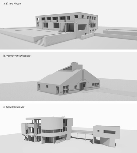
The logic for these hypotheses follows the traditional art-history model of aesthetic appreciation. The results are not, however, expected to be so straightforward, as the complexity of Postmodernism was not necessarily formal, it encompassed ideas and cultural iconography which are not measured using the present method. Furthermore, while Neo-modernism in general may have had moderate levels of complexity, Meier's work was celebrated for its rich formal modelling, suggesting it may not be typical of that style of work.

The following section describes the methodology used, the measures of visual complexity and attractive strength, and the~image processing approach. After this, this article reports the results of the measures for the three stylistic sets, including a series of descriptive, graphical and statistical results. Finally, this article concludes with a discussion about the limitations and implications of the methodology and results.

2. Methodology

2.1. Measuring visual complexity (fractal dimension)

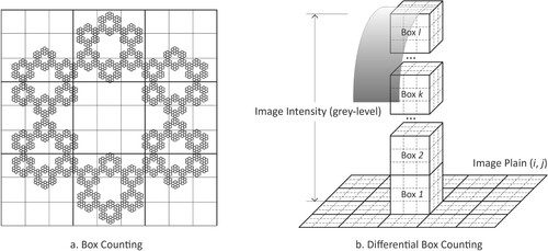
Fractal dimensions can be used to measure one important aspect of the aesthetic character of a building's façade, visual complexity. Complexity is significant because it is a predictor of preference, attractiveness, or beauty (Lee and Ostwald 2021). Fractal dimensions measure the distribution of data in a set, or in architectural applications, formal modelling in a plan or elevation (Bovill 1996; Lee and Ostwald 2021). The two-dimensional fractal analysis approach for building aesthetics commonly uses a box counting method because it is reliable and accurate (Batty and Longley 1994; Bovill 1996). However, there are other alternative approaches to measuring fractal dimensions (Lee and Ostwald 2021; Mandelbrot 1982). Importantly, a differential box counting method can determine the fractal dimensions of greyscale images. While the traditional box counting method has dominated architectural and urban research (Batty and Longley 1994; Bovill 1996; Ostwald and Vaughan 2016), it only works with binary images as shown in Figure 2a, which are not ideal for visual analysis. Thus, the present study uses the differential box counting method in Figure 2b because it can analyse greyscale images.

Figure 2. Grids and boxes of box counting and differential box counting.

The fractal dimension (D) of an image is: (1) $D=\underset{\epsilon \to 0}{lim}\frac{\log N_s}{\log (1/s)}$(1) where N_s is box count and s is box size. The differential box counting method, furthermore, takes into account an additional dimension (the third coordinate), image intensity, that is a grey-level ranging from 0 to 255 (Liu et al. 2014). As shown in Figure 2b, if the minimum and maximum grey-levels of a grid (i, j) fall in box number k and l, then the box counting is: (2) $n_s(i,j)=l-k+1$(2) The box counting measure, considering contributions from all blocks is: (3) $N_s=\sum n_s(i,j)$(3) The final D is the slope of the least square regression line (or trendline) for the log–log plot of N_s versus s, using the formula (1).

D values can be used to predict human visual preferences and examine visual complexity in design (Taylor 2001). Thus, in this article D is taken as a measure of the aesthetic character of visual attraction, i.e. visual complexity. Since the use of a different grid position can develop a slightly different D measures, four grid positions – four corners of the pixelated part of the image (the ‘bounding box’ or bbox) – are used and the four D values are then averaged.

For its calculations, this article uses an image analysis application (ImageJ) and a specialised plug-in (FracLac) originally developed for biology and physics (Karperien 1999-2013). In addition, this application of the box counting method uses the optimal settings identified in previous studies (Lee and Ostwald 2021; Ostwald and Vaughan 2016). The maximum grid size is 0.25 l where l is the height of the shorter side of bbox, while the minimum grid size is 10 pixels and the scaling coefficient is √2:1 (approximately, 1.4142:1).

2.2. Measuring attractive strength

Strength of attraction is calculated using visual attention data. Human visual processing is inherently selective and sequential, moving from one element to another over time (Suárez and Alfonso 2020). Recent eye-tracking technologies can capture participants’ visual movements and fixations in a gaze sequence map and a heatmap, respectively. The heatmap illustrates both the parts of an image that attract the subject's attention and the magnitude (e.g. duration) of fixation on these parts. ‘As interest in a stimulus increases, the eye tends to fixate more (i.e. increased fixation count) and for longer durations’ (Hollander et al. 2019, 159). Thus, the more attractive elements in the heatmap are depicted as intense warm colours, which indicate a longer fixation time. In contrast, non-coloured zones in the heatmap are ones which the participant ignores or doesn't directly look at. Likewise, visual attention software (VAS) algorithmically emulates human pre-attentive processing in vision (the initial 3–5 s of viewing and image) (3M 2021). The use of VAS overcomes several repeatability problems with eye tracking. Because VAS mimics human early vision and attention to visual elements (geometric edges, colour intensity, contrasts, and facial features relating to bilateral symmetry) heatmap data is directly comparable, allowing the properties of greyscale façade images to be measured and analysed.

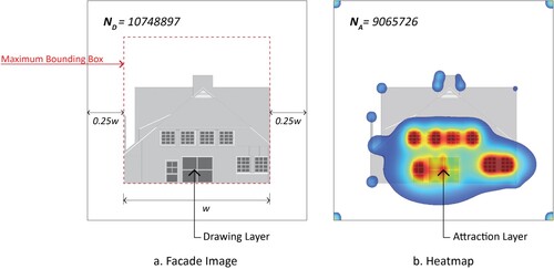
The logic behind the calculation of strength of attraction is as follows. Given the same viewing conditions (e.g. available time and extent of material/image), the heatmap of a more attractive façade will have more hot-coloured spots, but a smaller gross area of colour (fixated locations). Thus, the viewer is drawn to look very closely, or their gaze to linger longer, on particular points. A less attractive façade will have a larger area of colour, mostly cooler or blue in tone, as the eye drifts across it without being drawn to any particular location. Therefore, the attractive strength of a façade can be calculated by comparing data for the number of coloured pixels in a heatmap with the area of the image. That is, the gross area of attracted (or fixated) spots and the area of the elevation (not the entire image), are used to measure the magnitude of overlooking. Attractive strength is the reciprocal of the degree of overlooking (O). Thus, the attractive strength (S) is: (4) $S=\frac{1}{O}=\frac{N_D}{N_A}$(4) where N_A is the number of attraction layer pixels and N_D is the number of drawing layer pixels in an image. For example, the attractive strength (S) of the House in Delaware (east elevation) in Figure 3 is 10748897/9065726 = 1.1857. Because the eye may find little to fixate on in an unattractive façade, attractive strength (S) can be less than 1 (i.e. N_F may be larger than N_D).

Figure 3. (a) Drawing layer on an elevation image and (b) attraction layer on a heatmap of that image (House in Delaware by Robert Venturi with Denise Scott Brown).

2.3. Elevation image processing

This study uses façade images with a resolution of 4096 × 4096 pixels. In addition, since façade drawings are usually presented on white space, this image processing considers the acceptable white space (0.25w in Figure 3a) where w is the maximum width or height of an elevation drawing layer. In this article, w is 4096 pixels, and 0.25 w is 1024 pixels. Thus, the final image size is 6144 × 6144 pixels. Because some elevation drawings are wider or taller than others, this research considers the maximum bounding box in Figure 3a. In this way, all elevation images are consistently generated and analysed. The second important image processing step requires developing an appropriate level of representation for the attractiveness measures. Although there are multiple conventions to depict an architectural design, this research adopts Lee and Ostwald’s (2021) level 3 representation – an elevation drawing rendered with a light shade of grey (80% lightness) for the solid elements and a medium shade of grey (40% lightness) for openings as shown in Figure 3a – that is optimal for investigating both visual character and attention. There are several reasons for selecting these levels, but first it must be acknowledged that no greyscale representations of windows can capture their full characteristics in a consistent way. In reality, the houses examined in this article have different types of glass, which were produced in different areas and have diverse reflective properties. Indeed, early photos of the windows of Mies's Esters House show that from some angles, and under some weather conditions, they are almost completely transparent. However, in its renovated condition (from the mid 2000s), modern glazing was used, changing its visual characteristics. In a different way, some of Meier's buildings use double-glazing which, under many viewing conditions, appears as a silver, reflective surface. Past computational research (Ostwald and Vaughan 2016) has examined the impact of both ‘literal’ and ‘phenomenal’ transparency in façade openings on experimental results. The findings suggest that, rather than attempting to replicate diverse levels of transparency, opacity or reflectivity, which are largely reliant on factors external to the building (seasons, weather, time, era), it is more methodologically sound to use consistent greyscale levels. The levels of representation chosen for the present article reflect these standards and they are also in the ranges of typical greyscale renderings developed from the three buildings studied in this article. For example, the solid elements of the buildings in Figure 1 range from 60% to 85% lightness and their openings from 20% to 50% lightness. A façade image rendered with the two standard grey scales (80% and 40%) used in previous studies of this type is, therefore, acceptable for demonstrating a method.

2.4. Case selection and the optimal sub-set

The sample used to demonstrate the two methods comprises 60 elevations, four each from five Modernist, five Postmodernist and five Neo-modernist buildings. Each of the buildings in these three sets were produced by a major proponent of the style: respectively, Mies van der Rohe, Robert Venturi with Denise Scott Brown and Richard Meier. As stated previously, this is a deliberative sample of canonical works, which is used for demonstrating a method. It is acknowledged that this sample is not necessarily typical of the corpus of each style. Furthermore, canonical works were chosen over, say, vernacular works.

As the present article uses the three stylistic movements for demonstrating a method, extrapolation of results to a population mean isn't relevant and instead, pre-filtering the data is more important. For this reason, from the original 60 elevations an optimal sub-set is identified by removing elevations whose D values are out of the typical range (MEAN ± SD). For example, given the D range of the 20 Modern elevations (1.2971–1.3914), six are removed. In this way, the final optimal sub-set consists of 14 Modern, 13 Postmodern, and 12 Neo-modern elevations. Interestingly, all four elevations of the Postmodern Beach House were eliminated on this basis (see also Tables S1, S2, and S3 in the Supplementary Material).

3. Results

3.1. Attractiveness measures of the modern works

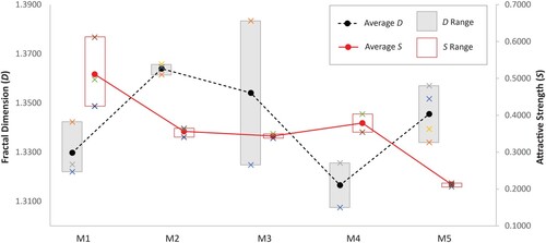
Five of Mies's Modern houses built between 1925 and 1951 are analysed in this section. The Wolf House (M1) was located on a hill in Gubin, Poland and destroyed in 1945. This early Modern brick house was a flat-roofed structure with multiple terraces. Like the other cases in this section, the design had a wide rectangular form. The Lange House (M2) and the Esters House (M3) share similar design and construction and are on adjacent sites in Krefeld. Both designs are similar in appearance to the Wolf House, although the latter works have a steel structure and larger openings. The last two houses are quite different in their functions and scales. The Lemke House (M4) was designed for both a home and gallery, while the Farnsworth House (M5) was intended for a weekend retreat. These single-storey buildings have a relatively simple design with very large windows (Lemke House) and glass walls (Farnsworth House).

Figure 4 illustrates the results with averages and ranges (see also Table S1 in the Supplementary Material). The lowest average D is for M4 (D = 1.3166) and the highest D for M2 (D = 1.3640), although the adjacent building (M3) also has a high value (D = 1.3541). The minimum D value in this set of 14 Modern elevations is for the E1 (north) of M4 (D = 1.3075) and the maximum D value is for the E2 of M3 (D  = 1.3834). As shown in Figure 4, there seems to be an inverse relationship between the average D and S values, but there is little or no relationship between individual D and S values. For example, the east elevations develop the highest average D, while they produce the second lowest average S (S = 0.3289). In contrast, the average D values of M5 is close to the average D of the Modern houses, while the last house has the lowest average S (S = 0.2125). The glass box design of M5 is responsible for the lowest S value in the set (E4 of M5, S = 0.2061) and the highest S value is for the E3 of M1 (S = 0.6115).

Figure 4. D and S values of Modernist houses with their averages and ranges.

3.2. Attractiveness measures of the postmodern works

Robert Venturi and Denise Scott Brown shared a passion for popularist iconography, rejecting minimalism in favour of designs that addressed cultural and historical cues. Five domestic designs (1959-1990) were chosen for the initial analysis in this article, the early works completed by Venturi alone, and the later with Scott Brown. However, as previously noted, the Beach House (P1) was removed in the initial data filtering. The Vanna Venturi House (P2) has a pitched roof, generating diagonal lines, and a chimney symmetrically at its centre, creating a strong visual focus. Its central entrance is also emphasised by an arch-framed decorative trim. The House in Vail (P3), which was built in 1977 as a ski-lodge, is located in Colorado. The four-storey tall and narrow building has a big arched dormer window on each side of its pyramid hip roof. The House in Delaware (P4) exhibits further expressive design elements. For example, a big arched screen is installed from the edges of the cross-gable roof, and a set of cookie-cut decorative columns from classical architecture deliver a playful appearance. The House on Long Island (P5) also has abstractions of Doric columns supporting a hipped roof with a big arched window. In summary, the use of hipped and gable roofs and over-sized, classical, or decorative design elements would appear to generate visual interest.

As expected, both the average D and S values of the four Postmodern houses, 1.3799 and 0.8082, respectively, are higher than those (1.3420 and 0.3604) of the Modern houses. As reported in Table S2, the lowest fractal dimension is for the E1 of P2 (D = 1.3057), and the highest is for E2 of P5 (D = 1.4293). The P5 is also the second most complex design in this Postmodern set, while the P2 is the least complex design. Interestingly, unlike the patterns of average D and S values in the Modern set (Figure 4), a positive relationship between average D and S values is visible in the Postmodern set (Figure 5).

Figure 5. D and S values of Postmodern houses with their averages and ranges.

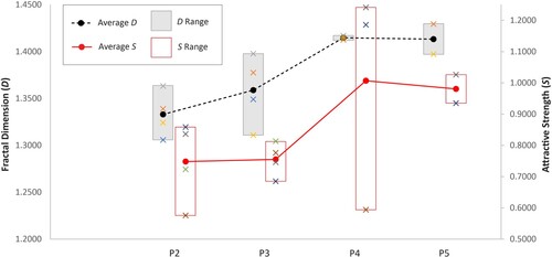
Notably, the S values of the Postmodern houses are higher than those of the Modern sample. The lowest S result is 0.5757 and the highest S is 1.2411. In contrast, all the S values of Modern elevations are lower than 0.5. The average S values of one pair of elevations (E1-North and E3-South) are quite lower than those of the other pair (E2-East and E4-West). This finding is interesting, because Venturi and Scott Brown frequently emphasised elements in the front and rear façades, which do not necessarily relate to one another. In this measure, the rhythmical openings (size and shape) on the side view of a cross-gable roof (E2 and E4) and a few protruding structures explain these differences. The over-sized parts and structures, such as a big arched window and a tall chimney, also increase the S values in the other cases (P2 and P3). That is, the S measure clearly identifies the attractiveness of individual architectural elements in the Postmodern set.

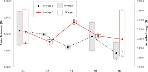
3.3. Attractiveness measures of the Neo-modernism houses

The five Meier houses were built from 1967 to 1974, being characterised as his ‘early designs’. These works celebrate geometric form, combining flat or curved planar walls with large openings, exposed chimneys, staircases, and entry bridges. Their appearance could be regarded as a type of exaggerated or maximal Modernism. The Smith House (N1), a weekend retreat, is characterised by a large glass wall and a roof terrace. It also has an entry bridge and a protruding staircase in the north-east and south-east elevations. Although the building does not adhere to a classic compass-based axis, the elevations are encoded as E1 and E2, respectively. The Hoffman House (N2) adopts double-height windows and a terrace. Like N1, a tall chimney develops a strong vertical structure in the elevation views. The Saltzman House (N3) consists of two separate buildings that are connected by an elevated bridge. The Douglas House (N4) looks down across the water of Harbour Springs. Since this building is on a steep hillside, the west elevation (E4), including a tall and exposed building foundation, is taller than the other elevations. Its appearance is characterised by rectangular glass walls with vertical and horizontal mullions, while a tall chimney, an entry bridge and an open staircase develop rich formal composition. Lastly, the Shamberg House (N5) appears to have a flat-roofed and simple rectangular form, with glass walls. This building also has an entry bridge and a protruding balcony.

As described in Table S3 in the Supplementary Material, the lowest average D is for N5 (D = 1.2970) and the highest D result for N2 (D = 1.3198). The average D result of N3 also indicates the lower complexity of its elevation design (D = 1.3043). Likewise, E1 of N5 has the lowest visual complexity (D = 1.2895) and E2 of N1 the highest (D = 1.3478). The average D and S values of the Neo-modern set has no correlation in Figure 6. For example, E2 of N1 has the highest D result, but its S value is lower than the average S value. E1 of N5 has the lowest D result, but its S value is the second highest S. in Figure 6. The lowest average S result is for the N2 (S = 0.5184), and the highest average S is for N3 (S = 0.7284). Likewise, the lowest S result is for E2 of N5 (S = 0.3662), and the highest S value is for E4 of N1 (S = 0.8653).

Figure 6. D and S values of Neo-modern houses with their averages and ranges.

3.4. Comparing D and S results

As hypothesised earlier in this article, the average D and S results of the Postmodernist façades (1.3721 and 0.8458, respectively) are higher than those of the Modernist façades (1.3432 and 0.3497, respectively). Furthermore, the average D and S results of the Neo-modern houses (1.3122 and 0.5973, respectively) fall between the other two styles. Figure 7 illustrates the results, and the differences between the three styles, in a scatter plot, representing D and S values. This graph indicates clear differences in attractive strength between Modern, Postmodern and Neo-modern houses.

Figure 7. A scatter plot of D and S values for 14 Modern, 13 Postmodern and 12 Neo-modern elevations.

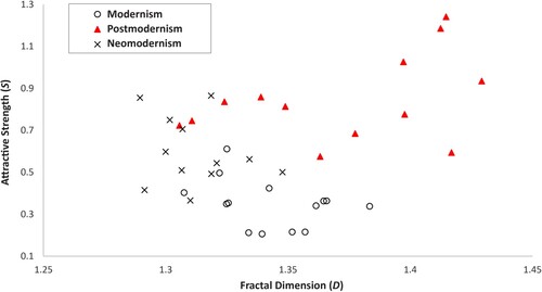
The lack of correlation between D and S is also, despite aesthetic theory and models, not unexpected. The fractal dimension is a holistic value of geometric or formal complexity, combining all of the parts and the whole. Attractive strength is focussed on the parts, often ignoring the whole. Thus, the two are measuring different types of ‘attractiveness’, which are more likely to be complementary than interconnected. Thus, the visual attractiveness of a building (A) may be the product of the two (D and S). If this simple model (A = D × S) is used, the visual attractiveness of the Postmodern set is 1.1605 and that of the Modern set is 0.4697. The A value of the Neo-modern set is 0.7838, which is between the other two, confirming the hypotheses of this article.

Statistically, by the one-way analysis of variance (ANOVA), there is a difference in fractal dimension at the p < 0.001 level for the three architectural styles, F(2, 36) = 12.847 as well as a significant difference in attractive strength at the p < 0.001 level, F(2, 36) = 30.719. As such, the D results of 13 Postmodern elevations (M = 1.3721, SD = 0.0430) compared to the Modern cases (M = 1.3432, SD = 0.0215) and the Neo-modern cases (M = 1.3122, SD = 0.0170) demonstrated significantly higher values, t(25) = 2.238, p = 0.034 and t(23) = 4.504, p = 0.000, respectively. The D results of 14 Modern elevations compared to the Neo-modern cases demonstrated significantly higher values, t(23.881) = 4.101, p = 0.000. Furthermore, the S results of Postmodern elevations (M = 0.8458, SD = 0.2053) compared to the Neo-modern cases (M = 0.5973, SD = 0.1629) demonstrated significantly higher values, t(22.523) = 3.365, p = 0.003. The S results of 12 Neo-modern elevations compared to the Modern cases (M = 0.3497, SD = 0.1159) also demonstrated significantly higher values, t(19.513) = 4.397, p = 0.000. Of course, the Postmodern elevations had higher S results compared to the Modern ones, t(18.652) = 7.653, p = 0.000.

These results suggest that both D and S measurements are useful for distinguishing one design style or appearance from the others in terms of attractiveness. In addition, the S measure tends to be shaped by the addition of visually interesting elements, such as the oversized chimney and large arched windows (see Figures S1, S2 and S3 in the Supplementary Material). These elements account for the higher S results in the Postmodern elevations. In summary, the optimal sub-set developed in the initial fractal analysis is useful for capturing significant differences in both visual complexity and attractive strength of the three architectural styles. Specifically, the results of attractive strength clearly confirm the hierarchical hypotheses of this article (Postmodernism > Neo-modernism > Modernism).

4. Discussion

4.1. An architectural attractiveness model

Following the application of these two methods to three sets of architectural images, it is possible to propose a new model of architectural attractiveness (A), which is the product of visual complexity (D) and attractive strength (S). This model combines measures derived from the geometry of a façade with its ‘intrinsic attractiveness’ (Frijda 1986). In the past, visual aesthetics has typically been examined in terms of partly opposing and partly complementary pairs of factors: ‘uniformity’ and ‘variety’, ‘concinnity’ (harmony) and ‘entropy’ (disorder), ‘coherence’ and ‘mystery’, and of course, ‘order’ and ‘complexity’ (Berlyne 1974). Of these pairs, order (or harmony) and complexity are commonly used to quantify the aesthetic value or character of a building façade (Meddahi and Boussora 2021; Ostwald and Vaughan 2016; Salingaros 1997). Importantly, since Berlyne's famous ‘inverted-U’ model (Berlyne 1971, 1974) of aesthetic appreciation, the relationship between complexity and preference in art appreciation has been an ongoing research topic (Althuizen 2021). However, Berlyne's model disregards the dynamic nature of ‘aesthetic episodes’ and the many separate factors that also affect aesthetic judgment (Jacobsen and Höfel 2002). As just one example, symmetry clearly catches the eye in a particular way (Locher and Nodine 1987). Drawing on aspects of this previous research, the present article defines architectural attractiveness as a product of visual complexity, a primary factor of visual attractiveness, and attractive strength, a composite measure of several factors (e.g. intensity, contrast, and symmetry), in the context of the formal properties of a building façade.

This new attractiveness model is also potentially valuable for examining stimulus-sensation responses and the relationship between complexity, preference, and evaluation. For example, Stamp's (1999) façade preference experiment quantifies three types of visual stimuli (silhouette complexity, surface complexity, and façade articulation), whilst human visual preferences are measured by respondents’ ratings. In another study on visual diversity (Stamps 2003), the visual entropy of a design is shown to have a relationship with participants’ responses on semantic differential scales of pleasant/unpleasant and diverse/uniform. Since visual stimuli and levels of complexity are related to the visual attractiveness of a façade design, past research has repeatedly focused on the complexity of physical design elements (Meddahi and Boussora 2021; Stamps 1999, 2003). Such research suggests that the visual complexity of a façade is an important indicator of its aesthetic character. In contrast, the power of holding a person's gaze is a measure of attractiveness or ‘interestingness’ (Grabner et al. 2013). Khalighy et al. (2015) quantified the qualities of beauty and attractiveness using eye-tracking in product design. In their study, pureness is ‘1/number of fixations’ and proportion is ‘1/standard deviation of duration of fixations’. These variables – pureness, proportion, contrast, appropriateness, and novelty – can be used for calculating the qualities of an object and collectively determining its attractiveness. Since there are no architectural precedents for quantitatively examining attractive strength, the present research proposes a new measure (S) based on pre-attentive processing in vision. Significantly, the S measure also encapsulates ‘architectural temperature’ (T) from Klinger's and Salingaros's model (1997) where the emotional perception of a building design (L) is the production of architectural temperature (T) and harmony (H). Although the architectural temperature model addresses a building's emotional impact, the concept of ‘harmony’ or ‘order’ usefully articulate the architectural attractiveness model.

4.2. Visual representation

In this article, the visual complexity (D) of greyscale façade images are measured using the differential box counting method. As acknowledged previously, that actual visual experience of an architectural façade in the real word is shaped by many factors (colours, materials, textures and even biophilic design elements), the experience of which changes in response to the viewer's location or movement in space. Furthermore, the perception of these design factors or elements is reliant on external variables such as weather and lighting conditions. While limited in some ways, the 2D greyscale renderings used in this article offer a controlled, and thereby repeatable, set of experimental conditions, by removing more diverse three-dimensional, phenomenologically dominated, and contingent spatio-visual experience. This is both a strength and a weakness of the method, although for developing a theoretical or conceptual examination of the topic, the chosen parameters are the most viable ones.

In a similar way, it is worth noting that the D value of a greyscale rendering is valuable because it provides a universal measure of ‘geometric complexity’, which is neither impacted by, nor captures, participants’ diverse social and cultural backgrounds or emotional states. Furthermore, past research has examined multiple levels of graphic representation of architecture (Lee and Ostwald 2021) finding that fractal dimensions of greyscale images are amongst the most useful and repeatable measures for studies of aesthetic experience at an early design stage. Whilst it might, methodologically, be difficult to consider heterogeneous design factors in the visual representation of a façade, one promising alternative would be taking colour into consideration. Certainly, it is possible to measure the fractal dimension of colour renderings, using an extended differential box counting method (Nayak et al. 2018). Such a method, however, still analyses greyscale data extracted from RGB images, but it may be a superior option for identifying the visual complexity of a façade. Colour-rendered images are also able to be examined using VAS because it accommodates colour contrasts (‘red-green’ and ‘blue-yellow’) (Lee and Ostwald 2021). Regardless of this capacity, even if a colour-rendering might be considered an appropriate representation for this purpose, colour itself is a culturally sensitive factor and dependent on many external variables. Colour is, significantly, neither fixed nor universal as individuals see colour differently. This is also why the vast majority of previous studies of this type in architecture have used binary (Batty and Longley 1994; Bovill 1996; Ostwald and Vaughan 2016) or greyscale images (Lee and Ostwald 2021; Liu et al. 2014; Mandelbrot 1982), to focus on ‘geometric complexity’ or ‘formal complexity’ which can be measured in consistent and repeatable ways. Nonetheless, a future study could examine the architectural attractiveness (D × S) of a colour rendering.

4.3. Visual attention simulation

In order to measure the attractive strength (S) of a building, this article has focused on the pre-attentive vision that is algorithmically captured by VAS. This method has been applied in the fields of architecture and urban design (Hollander et al. 2021; Milliken et al. 2021; Salingaros and Sussman 2020), because it is more efficient (Hollander et al. 2021), and for many purposes, as reliable and effective as eye tracking hardware (3M 2021). While VAS can predict pre-attentive vision with 92% accuracy (3M 2021), validation studies have revealed that 3M VAS predictive efficiency ranges from 85% to 94% when disregarding fixation biases (3M Commercial Graphics Division 2022). However, VAS only works for the pre-attentive vision. Thus, conventional eye-tracking studies are still necessary for conscious visual attention. Advances in technology have made eye-tracking hardware increasingly accessible for researchers, although its use is time consuming, test – retest reliability can be problematic, and the resulting data is often presented and analysed qualitatively (Suárez and Alfonso 2020; Hollander et al. 2020). Both VAS and eye-tracking can be used to measure visual attention, particularly, the power of holding a person's gaze, which is a measure of attractiveness or ‘interestingness’ (Grabner et al. 2013). Furthermore, VAS has been used to examine the relationship between visual stimuli and human visual processing of a building façade, revealing that visual complexity has a relationship with pre-attentive vision (Lee and Ostwald 2021). In this way, VAS can be regarded as an alternative way of examining ‘early vision’ (Rensink 2000) or the ‘stimulus-sensation relationship in design’ (Lee and Ostwald 2021).

5. Conclusion

This article has introduced two computational measures of architectural visual attractiveness, visual complexity (measured using fractal dimensions) and attractive strength (measured using visual attention simulation). These are computational methods that have been used for different types of spatial and formal analysis in the past. The results in this article indicate that these computational methodologies can contribute to quantitatively investigating the attractive properties of architectural façades. Furthermore, the comparative analysis in this article suggests that, on average, each style was mathematically differentiable with varying degrees of statistical significance. There are, however, multiple limitations to these methods and the results.

Although this article used the differential box counting method, which can capture the textual intensity of an image, the D results are still confined to recording geometric complexities. Despite the results of past studies correlating D to aesthetic appreciation, formal complexity is not, in isolation, a perfect way of differentiating style or measuring attraction. Nevertheless, both D and S measures do identify differences in the visual attractiveness of the three styles, which is a new contribution to disciplinary knowledge. Conversely, there is no mathematical correlation between D and S, even though they may both separately fulfil their purposes. Thus, being engaging (visual complexity) and appealing (attractive strength) may not be connected. A future study will examine the proposed model (A = D × S), as a predictor of visual attractiveness, with a subjective report as well as an extended sample size.

Finally, the visual attractiveness of a building is one of the most influential factors that shape people's perceptions of a city or place. As such, examining the visual consequences of architecture at the early design stage is an important issue for the built environment. Importantly, both D and S values are limited to the innate measures of visual complexity and attractive strength – in other words, geometric complexity and pre-attentive strength – which shape an immediate human response to architecture. As discussed, this intuitive response wouldn't be influenced by cultural and contextual factors. Acknowledging that a building is never ‘stand-alone’ and from a stylistic perspective the concept of ‘attractiveness’ can change over time, the methodology and tools introduced in this article can be used to measure one distinct type of aesthetic attraction, and also be used by diverse stakeholders in this field. In addition, this article has presented two tangible, computational tools that can be applied to assess completed designs as well as design variations where visual attractiveness is a required criterion. Collectively, this article contributes to architectural design research and practice.

Disclosure statement

No potential conflict of interest was reported by the author(s).

Additional information

Funding

This research was supported by the ARC (DP220101598), UNSW Scientia program, and an ADA Fellowship at UNSW Sydney.

References

- 3M. 2021. ‘How does VAS work and what is first-glance vision?’, accessed 8 February. https://vas.3m.com/support.
- 3M Commercial Graphics Division. 2022. “3M Visual Attention Service Validation Study.” 3M Corporation, Accessed 23 August 2022. https://multimedia.3m.com/mws/media/1006827O/3msm-visual-attention-software-vas-validation-study.pdf?fn=VAS_%20Validation%20Study.pdf.
- Althuizen, Niek. 2021. “Revisiting Berlyne’s Inverted U-Shape Relationship Between Complexity and Liking: The Role of Effort, Arousal, and Status in the Appreciation of Product Design Aesthetics.” Psychology & Marketing 38 (3): 481–503. doi:10.1002/mar.21449.
- Arnheim, Rudolf. 1966. Toward a Psychology of Art. Berkeley, CA: Univ. of California Press.
- Batty, Michael, and Paul A Longley. 1994. Fractal Cities: A Geometry of Form and Function. New York: Academic press.
- Berlyne, Daniel E. 1971. Aesthetics and Psychobiology. New York, NY: Appleton-Century-Crofts.
- Berlyne, Daniel E. 1974. Studies in the New Experimental Aesthetics: Steps toward an Objective Psychology of Aesthetic Appreciation. Washington: Hemisphere Pub. Corp.
- Berscheid, Ellen, and Elaine Walster. 1974. “Physical Attractiveness.” In Advances in Experimental Social Psychology, edited by Leonard Berkowitz, 157–215. New York: Academic Press.
- Bovill, Carl. 1996. Fractal Geometry in Architecture and Design. Boston: Birkhäuser.
- Bower, Isabella, Richard Tucker, and Peter G. Enticott. 2019. “Impact of Built Environment Design on Emotion Measured via Neurophysiological Correlates and Subjective Indicators: A Systematic Review.” Journal of Environmental Psychology 66: 101344. doi:10.1016/j.jenvp.2019.101344.
- Cambridge University Press. n.d. ‘Attractiveness.’ Cambridge Dictionary, accessed 4 April. https://dictionary.cambridge.org/dictionary/english/attractiveness.
- Cupchik, Gerald C. 1986. “A Decade after Berlyne.” Poetics 15 (4): 345–369. doi:10.1016/0304-422X(86)90003-3.
- Frijda, Nico H. 1986. The Emotions. Cambridge, UK: Cambridge University Press.
- Giese, Joan L., Keven Malkewitz, Ulrich R. Orth, and Pamela W. Henderson. 2014. “Advancing the Aesthetic Middle Principle: Trade-Offs in Design Attractiveness and Strength.” Journal of Business Research 67 (6): 1154–1161. doi:10.1016/j.jbusres.2013.05.018.
- Grabner, Helmut, Fabian Nater, Michel Druey, and Luc Van Gool. 2013. “Visual Interestingness in Image Sequences.” Proceedings of the 21st ACM international conference on multimedia, 1017–1026, Barcelona, Spain: Association for Computing Machinery.
- Hollander, Justin B., and Eric C. Anderson. 2020. “The Impact of Urban Façade Quality on Affective Feelings.” Archnet-IJAR: International Journal of Architectural Research ahead-of-print (2): 219–232. doi:10.1108/ARCH-07-2019-0181.
- Hollander, Justin B., Alexandra Purdy, Andrew Wiley, Veronica Foster, Robert J. K. Jacob, Holly A. Taylor, and Tad T. Brunyé. 2019. “Seeing the City: Using Eye-Tracking Technology to Explore Cognitive Responses to the Built Environment.” Journal of Urbanism: International Research on Placemaking and Urban Sustainability 12 (2): 156–171. doi:10.1080/17549175.2018.1531908.
- Hollander, Justin B., Ann Sussman, Alex Purdy Levering, and Cara Foster-Karim. 2020. “Using Eye-Tracking to Understand Human Responses to Traditional Neighborhood Designs.” Planning Practice & Research 35 (5): 485–509. doi:10.1080/02697459.2020.1768332.
- Hollander, Justin B., Ann Sussman, Peter Lowitt, Neil Angus, and Minyu Situ. 2021. “Eye-Tracking Emulation Software: A Promising Urban Design Tool.” Architectural Science Review, 383–393. doi:10.1080/00038628.2021.1929055.
- Jacobsen, Thomas, and Lea Höfel. 2002. “Aesthetic Judgments of Novel Graphic Patterns: Analyses of Individual Judgments.” Perceptual and Motor Skills 95 (3): 755–766. doi:10.2466/pms.2002.95.3.755.
- Karperien, Audrey. 1999-2013. ‘Fraclac for imagej.’ accessed 15 Feb. http://rsb.info.nih.gov/ij/plugins/fraclac/FLHelp/Introduction.htm.
- Khalighy, Shahabeddin, Graham Green, Christoph Scheepers, and Craig Whittet. 2015. “Quantifying the Qualities of Aesthetics in Product Design Using Eye-Tracking Technology.” International Journal of Industrial Ergonomics 49: 31–43. doi:10.1016/j.ergon.2015.05.011.
- Kozlowski, Marek. 2007. Urban Design: Shaping Attractiveness of the Urban Environment with the End-Users.’ PhD Thesis, School of Geography, Planning and Architecture, University of Queensland.
- Leder, Helmut, and Marcos Nadal. 2014. “Ten Years of a Model of Aesthetic Appreciation and Aesthetic Judgments : The Aesthetic Episode - Developments and Challenges in Empirical Aesthetics.” British Journal of Psychology 105 (4): 443–464. doi:10.1111/bjop.12084.
- Lee, Ju Hyun, and Michael J. Ostwald. 2021. “Fractal Dimension Calculation and Visual Attention Simulation: Assessing the Visual Character of an Architectural Façade.” Buildings 11 (4): 163.
- Locher, Paul J., and Calvin F. Nodine. 1987. “Symmetry Catches the Eye.” In Eye Movements from Physiology to Cognition, edited by J. K. O’Regan, and A. Levy-Schoen, 353–361. Amsterdam: Elsevier.
- Lynch, Kevin. 1960. The Image of the City. Cambridge, MA: The MIT Press.
- Mandelbrot, Benoit B. 1982. The Fractal Geometry of Nature. New York: WH freeman.
- Meddahi, Kahina, and Kenza Boussora. 2021. “Aesthetic Measures of Algiers’ Colonial Facades.” Nexus Network Journal, doi:10.1007/s00004-021-00546-z.
- Merriam-Webster. n.d. ‘Attractiveness.’ Merriam-Webster.com Thesaurus, accessed 4 April. https://www.merriam-webster.com/thesaurus/attrac-tiveness.
- Milliken, Peter, Justin B. Hollander, Ann Sussman, and Minyu Situ. 2021. “Identifying Biophilic Design Elements in Streetscapes: A Study of Visual Attention and Sense of Place.” In Urban Experience and Design: Contemporary Perspectives on Improving the Public Realm, edited by Justin B. Hollander, and Ann Sussman, 75–90. New York: Routledge.
- Nasar, Jack L. 1994. “Urban Design Aesthetics.” Environment and Behavior 26 (3): 377–401. doi:10.1177/001391659402600305.
- Nayak, Soumya Ranjan, Jibitesh Mishra, Asimananda Khandual, andGopinath Palai. 2018. “Fractal Dimension of RGB Color Images.” Optik 162: 196–205. doi:10.1016/j.ijleo.2018.02.066.
- Ostwald, Michael J., and Josephine Vaughan. 2016. The Fractal Dimension of Architecture. Cham, Switzerland: Birkhäuser.
- Rensink, Ronald A. 2000. “The Dynamic Representation of Scenes.” Visual Cognition 7 (1-3): 17–42. doi:10.1080/135062800394667.
- Salingaros, N. A. 1997. “Life and Complexity in Architecture from a Thermodynamic Analogy.” Physics Essays 10: 165–173.
- Salingaros, N. A., and A. Sussman. 2020. “Biometric Pilot-Studies Reveal the Arrangement and Shape of Windows on a Traditional Façade to be Implicitly “Engaging”, Whereas Contemporary Façades are Not.” Urban Science 4 (5): 26.
- Stamps, Arthur E. 1999. “Physical Determinants of Preferences for Residential Facades.” Environment and Behavior 31 (6): 723–751. doi:10.1177/001391-69921972326.
- Stamps, Arthur E. 2000. Psychology and the Aesthetics of the Built Environment, Environment and Behavior. Boston, MA: Kluwer Academic.
- Stamps, Arthur E. 2003. “Advances in Visual Diversity and Entropy.” Environment and Planning B: Planning and Design 30 (3): 449–463. doi:10.1068/b12986.
- Suárez, de la Fuente, and Luis Alfonso. 2020. “Subjective Experience and Visual Attention to a Historic Building: A Real-World eye-Tracking Study.” Frontiers of Architectural Research 9 (4): 774–804. doi:10.1016/j.foar.2020.07.006.
- Taylor, Richard. 2001. “Science in Culture.” Nature 410 (6824): 18–18. doi:10.1038/35065154.
- Venturi, Robert. 1965. “Complexity and Contradiction in Architecture: Selections from a Forthcoming Book.” Perspecta 9/10: 17–56.