Fibre optic sensors based on hollow capillary tube with three tightly encapsulated optical fibres

Abstract

Fibre optic sensor cable technology is relatively a new research area that combines a set of scientific and technical disciplines in order to meet distributed sensor system needs and quality standards. In this paper, we discuss a fibre optic sensor design with three tightly encapsulated fibres for multipurpose and multivalent sensing. It has the potential to integrate more detection and measurement techniques into a small space, and this, in turn, largely contributes to installation and cost optimizations and directly impacts investment plans and industrial success. The developed cable is tested in a specially developed high pressure and high temperature chamber. Furthermore, it is demonstrated that the proposed sensor cable offers the possibility of detection and distributed measurement of temperature, pressure, bending and vibrations.

KEYWORDS:

• Optical fibre
• fibre optic measurements
• monitoring systems
• fully distributed optical fibre sensor
• acoustic sensors
• strain sensors
• temperature sensors
• pressure sensors
• Brillouin effect
• Brillouin Optical Time Domain Analysis (BOTDA)

1. Introduction

Massive digitalization of physical objects and infrastructure as a part of Internet of Things (IoT) systems is the industry of the twenty-first century. The considered systems and solutions are based on either wireline or wireless systems and on combination of the two. Among these approaches there are few different technologies using photonic phenomena and employing optical fibres and cables of different types and sizes such as measurement probes and sensors providing detection and measurement data from each segment in the length. They are referred to as distributed fibre optic sensors. As such they add contribution to these digitalization efforts especially in cases when measurement can be conducted only from one end of long linear asset, i.e. some infrastructural object such as pipeline or underground duct system. Since detection and measurement regime is distributed – and their costs are considered per-metre or per-kilometre the optical fibre sensing systems offer unmatched price-performance ratio. This is the reason for their growing success in the industry and that they have become the essential digitalization tool in energy discovery, production and transportation. The examples of this are: distributed temperature sensor (DTS), distributed temperature and strain sensor (DTSS) and distributed acoustic sensor (DAS) systems [1–5]. Their further advantages are related to high sensitivity, electromagnetic and galvanic immunity, small size and weight, etc.

Engineering challenges on both sensor and system design are how to meet strict industrial and environmental standards. It starts with material composition and selection, sensor construction, manufacturing processes and testing methods and procedures. This results in need for constant improvements and specialization in all: sensing optical fibre, sensor cable design, interrogation hardware, as well as in signal processing, interpretation and visualization techniques. On the one hand, smart design of optical fibre and cable constructions can dramatically impact and reduce development time and complexity in the upper layers of the measurement system, such as the one in optical and signal processing layer, on the other hand, system designers must be aware of the system applicability on sites. This is especially true for sensing cables as they are set in contact with physical environment and quantities that are referred to as measurands. Working on the deployment sites in many cases involves harsh and extreme conditions. The best examples are geophysical and civil construction sites in which open optical fibres are exposed to water, hydrogen-rich chemicals and mechanical stress. Therefore, they differ largely from laboratory conditions in which the systems are conceptualized and constructed. The manipulation of fibre optic sensing cables that include working with sensitive optical fibres under such circumstances presents a constant challenge, and it very often requires special skills and experience from the technicians. The designers of sensor interrogation equipment, cables and application solutions must be aware of their applicability on sites.

This paper presents and discusses a unique sensor cable design [6], branded and introduced in the industry under the name “Trisens”, which is presently used in the industry in distributed strain and acoustic measurements. Furthermore, it will be shown that this concept has the potential to be deployed in distributed pressure measurements as well, for example, by means of birefringence change techniques [7–9] that is generated using common standard symmetrical industrial raw materials in the cable manufacturing industry. Hence, the sensor cable is aimed for multipurpose and configuration multivalent distributed optical fibre sensing.

2. Optical fibre sensor cable with three tightly encapsulated optical fibres

Stainless steel tubing (SST) in its various forms has been traditionally used for production of optical power ground wire where it has been used for telecommunication exchange in power transmission systems, i.e. in overhead power lines. Nevertheless, this tubing has been proved also to provide a quality protection for fragile and sensitive optical fibres in other environments and applications, such as measurement and sensing in harsh environments. Because of its metallic nature SST exhibits intrinsically large thermal conductivity assuring easy and fast thermal energy transmission through the walls of the SST. Another advantage is that optical fibres enclosed in the SST – now called Fiber in Metal Tube (FIMT) – can survive harsh environment conditions, such as in aggressive chemical and mechanically demanding conditions. This counts especially for down-hole applications where pressure can reach beyond 900 bar, and temperatures reach 350°C.

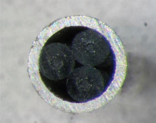
The proposed sensor cable consists of three optical fibres (Figure 1), positioned at 120° in a cross-section azimuthal plain and tightly encapsulated in a metal tubing by means of FIMT production machinery using laser welding technique. Tight encapsulation here means that all fibres are in physical contact with metal tubing on top. The amount of physical contact in terms of pressure between optical fibres and inner wall of metallic tubing can be regulated during the production process. The basic idea for this design is to arrange tight-buffer construction producible in long lengths with three fibres. All three fibres must be in just optimum contact with steel encapsulation on top of it.

Figure 1. Cable prototype with overall OD 1.25 mm.

Information on the quality of contact and all other parameters can be obtained from various measurements. Two techniques are particularly useful. The most essential data can be gained from Rayleigh backscattering using Optical Time Domain Reflectometry (OTDR). The others are acoustics-phonon measurement techniques such as Brillouin Optical Time Domain Analysis (BOTDA) and Brillouin Optical Time Doman Reflectometry (BOTDR) measurements [10,11]. From the pressure sensing point of view the configuration and mechanical-optical properties are the most important ones. In order to assure change in birefringence in dependence of the external pressure the configuration needs to provide asymmetrical load exerted on each fibre as a result of external pressure on the encapsulation tube, as depicted in Figure 2.

Figure 2. Concept of a sensor cable based on three optical fibres encapsulated in a metal or plastic jacket; (a) cable design, (b) configuration of forces exerted on optical fibre.

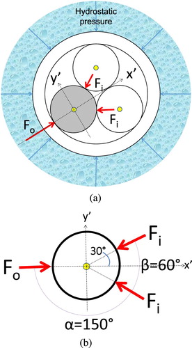
The fibre under consideration is fixed and “sandwiched” into the position by surrounding encapsulation tubing and two other adjacent fibres. Thus, it shall see three forces exerted on its circumference; one from encapsulation tubing and one from each adjacent fibre. Consequently, in static equilibrium we will have: (1) $\begin{array}{c}\sum _i{F}_{xi}=0;\sum _i{F}_{yi}=0\end{array}$(1) For the x′-axis we have: (2) $\begin{array}{c}{F}_o-2F_i\cos ({30}^{\circ })=0\end{array}$(2) (3) $\begin{array}{c}{F}_o=\sqrt{3}{F}_i\end{array}$(3) The same analysis approach for y′-axis gives: (4) $\begin{array}{c}0+F_i\sin ({30}^{\circ })-F_i\sin ({30}^{\circ })=0\end{array}$(4) Because $F_o=\sqrt{3}{F}_i$, the fibre is consequently asymmetrically loaded. This gives rise to birefringence in the core of the optical fibre. In this way the birefringence as asymmetrical phenomenon is generated by means of symmetrical elements that are easily available on the market.

2.1. Validation with finite element method (FEM)

This concept can be validated using FEA - Finite Element Analysis. For this purpose, Abaqus FEA simulation software is used [12]. There are few parameters that need to be defined and mesh set for the analysis. The analysis is made on a relatively large design (Figure 3) having outer diameter (OD) of 2.213 mm and wall thickness (WT) of approximately 0.25 mm. Young modulus $(E)$ and Poisson ratio $(v)$ along with other parameters and information of interest are:

1. Material properties used for FEM

   1. Steel: E = 210 GPa, ν = 0.30

   2. Polymer: E = 2.7 GPa, ν = 0.34

2. Loads: static pressure, magnitude up to 1200 bars

3. Finite element type: plane strain, quadratic, reduced integration (CPE8R)

4. Evaluated parameters

   1. Inner diameter changes of steel tube (delta Rx, delta Ry)

   2. Outer diameter changes of optical fibre (delta Rx, delta Ry, delta R_30°/90°/150°)

Figure 3. Validation using Finite Element Method (FEM) applied to the cable; (a) the geometry with dimensions, (b) the FEM mesh configuration with legend showing the pressure magnitudes in TPa, (c) change in inner diameter, and (d) radial deformation due to asymmetrical loading obtained at the observed azimuthal angles. The diameter changes for the fibre-1 at angles 30°, 90 and 150° are −0.001659, 0.00168 and 0.00165 μm, respectively.

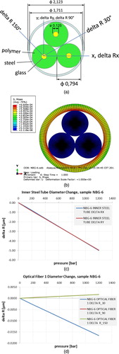
As it can be seen from the obtained results showing change in radius of the encapsulation tube and optical fibre-1, FEM analysis confirms the assumption of asymmetrical loading and gives insight in magnitudes of the effect for the hydrostatic pressure up to 1200 bar for the materials used. Due to the pressure increase and consequent asymmetrical loading, each optical fibre compresses at the angle of 30°, and extends at 90° and 150°. Note that the considered angles 90° and 150° are between the angles for which the fibre 1 is in contact with the metal tube and with the other fibres inside the tube (0° and 60°, respectively).

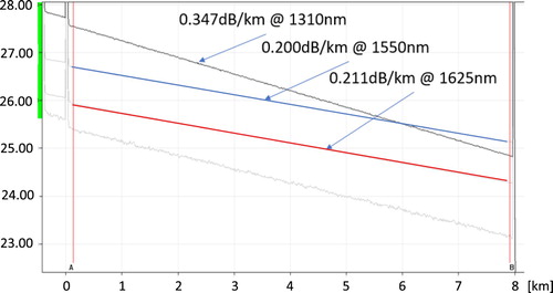
From the optical performance point of view, it is crucial that design can be manufactured without introduction of additional losses yet with enough contact between the steel tube and optical fibres inside. Figure 4 shows good practice and losses within acceptable range comparable with the bare fibre. The measurements are done using Exfo FTB-500 test platform show average attenuation of 0.347 dB/km at 1310 nm and 0.20 dB/km at 1550 nm and 0.211 at 1625 nm from all three fibres, respectively.

Figure 4. Characteristic losses obtained from all the fibres of the prototype, each at different wavelength.

3. Stainless steel tube in high pressure environment

It was of interest to evaluate the behaviour of the SST when subjected to high hydrostatic pressure, i.e. to experimentally prove the FEM calculations. With this objective in mind, it was realized there is necessity to build high pressure and high temperature chamber aimed for both optical and mechanical measurements, and characterization of optical fibres and FIMTs. The details of pressure chamber are provided in [13]. Since its length exceeds 24 m, all relevant resolution lengths in distributed optical sensing are supported by the design. The pressure chamber is particularly useful for simulation of borehole conditions. For example, using this test chamber the collapse pressure of the samples can be determined as a measure of precision in the manufacturing process. The collapse pressure is inversely proportional to the ellipticity of the sample under test and to the ratio between OD and wall thickness.

Let us demonstrate the possibilities of developed chamber on an example of measuring compression magnitude of sensor cable and its repeatability in the pressure cycling. The sample is filled with water and brought through the pressure chamber and sealed on both ends (Figure 5).

Figure 5. Measurement of the change in tube’s outer and inner diameters under high pressure (a) Evaluation set-up; (b) measurement results.

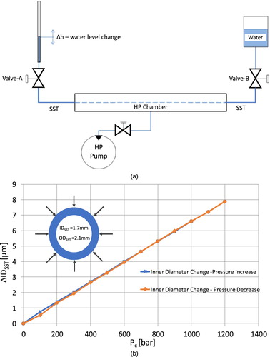
The water tank is installed on the right end of the sample, whereas the water level indicator is placed to its left terminal. Both ends of the sample are led outside the pressure chamber and thus they are freed from the pressure impact. The water is then led through the sample all the way to the water indicator on the other side. The tank valve is then closed, and water reference level indicated. Once the pressure chamber is pressurized in the chamber the sample compresses and water inside the sample can escape now only to the left side and the water level in the indicator follows the change in cable diameter. The reduction in both inner and outer diameters of sample due to compression has been observed and measured. The change in water level due to pressure increase shall be (5) $\begin{array}{rl}{\left(\frac{I{D}_{IND}}{2}\right)}^2\pi \Delta h& ={\left(\frac{I{D}_{SST}}{2}\right)}^2\pi L_{CH}\\ & -{\left(\frac{I{D}_{SST}-\Delta I{D}_{SST}}{2}\right)}^2\pi L_{CH}\end{array}$(5) (6) $\begin{array}{rl}\mathrm{\Delta }h& =\frac{\mathrm{\Delta }I{D}_{SST}(2I{D}_{SST}-\mathrm{\Delta }I{D}_{SST})}{I{D}_{IND}^2}\end{array}$(6) From this equation ΔID_SST can be extracted: (7) $\mathrm{\Delta }I{D}_{SST}=I{D}_{SST}\left(1-\sqrt{1-\frac{\mathrm{\Delta }h}{L_{CH}}{\left(\frac{I{D}_{IND}}{I{D}_{SST}}\right)}^2}\right)$(7) where

• Δh is the water level change due to pressure change in the indicator

• ΔID_SST is the change in the inner diameter of the steel tube

• ID_SST is the initial inner diameter of the steel tube

• ID_IND is the inner diameter of water level indicator

• L_CH is the effective pressure chamber length

The obtained results qualify stainless steel tube for the purpose of distributed pressure measurements within the pressure range from 0 to 1200 bar. One very important detail is to be noticed here: the SST acts here also as a pressure transducer, scaling the pressure to the range that assures long term integrity and lifetime of the optical fibre. All this yields a range of possibilities for further optimization techniques that shall be discussed later.

4. Stimulated Brillouin scattering measurements

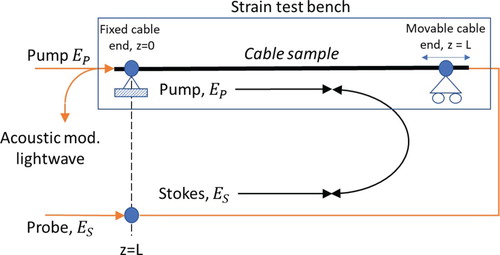
The fibre optic cable is interrogated with stimulated Brillouin scattering measurement technique more precisely with BOTDA system [14]. The measurement set-up is shown in Figure 6. The intensity of pumped and Stokes optical signals (I_P and I_S) can be described with the following differential equations [15]: (8) $\begin{array}{rl}\left[\frac{n}{c}\frac{\mathrm{\partial }}{\mathrm{\partial }t}-\frac{\mathrm{\partial }}{\mathrm{\partial }z}+\alpha \right]I_P& =-\gamma g_B{I}_S{I}_P\end{array}$(8) (9) $\begin{array}{rl}\left[\frac{n}{c}\frac{\mathrm{\partial }}{\mathrm{\partial }t}-\frac{\mathrm{\partial }}{\mathrm{\partial }z}+\alpha \right]I_S& =\gamma g_B{I}_S{I}_P\end{array}$(9) where

• $I_P$ intensity of the pump

• $I_S$ intensity of the Stokes scanning light

• $\gamma$ polarization efficiency

• $g_B$ gain of Brillouin stimulated emission

• $\alpha$ characteristic attenuation

Figure 6. Typical stimulated Brillouin measurement set-up for strain testing and characterization.

The birefringence properties along the fibre impact polarization states of waves propagating along the fibre and this is taken into account by polarization-dependent amplification factor γ [15] that multiplies Brillouin gain g_B. The change in the birefringence impacts the difference in propagation constant of two characteristic waves $\mathrm{\Delta }k$ that changes γ as follows (10) $\begin{array}{rl}\gamma (z)& =\frac{1}{2}[co{s}^2({\alpha }_S-{\alpha }_P)-co{s}^2({\alpha }_S+{\alpha }_P)]\\ & \times [1+cos[2\mathrm{\Delta }kz-\mathrm{\Delta }kL+2({\delta }_S-{\delta }_P)]\\ & +co{s}^2({\alpha }_S+{\alpha }_P)]\end{array}$(10) The Brillouin gain can be described with (11) $\begin{array}{rl}{g}_B& =g_{B0}\frac{1}{1+4\left(\frac{f_D-f_B}{\mathrm{\Delta }{f}_B}\right)}\end{array}$(11) (12) $\begin{array}{rl}{g}_{B0}& =\frac{2{\pi }^2{n}^7{p}_{12}^2}{c{\lambda }^2{\varrho }_0{\gamma }_S{c}_S}\end{array}$(12) where

• $n$ refractive index

• $c$ speed of light

• $\lambda$ wavelength in vacuum

• $p_{12}^{}$ electrostriction coefficient

• ${\varrho }_0$ mass density

• ${\gamma }_S$ acoustic attenuation coefficient

• $c_S$ speed of the acoustic wave

4.1. Strain measurements

The SBS interrogation of optical fibres and cables involves two counter-propagating lights and it means that optical fibre loop must be arranged. Figure 6 shows typical configuration for characterization of strain properties. There are two ports from which the light waves are launched; pump port and Stokes port. The pump wave is pulsed in order to provide spatial profiling and Stokes wave is a tunable continues light wave providing scanning of the spectral range in which Brillouin effect takes place. The cable sample is inserted within the half that is closer to the pump port. This is efficient since the pump in that segment is non-depleted and more pump power is converted and invested into the Brillouin interaction and generation of acoustic wave.

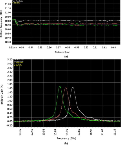
The analysis of the SBS backscatter involves profiling of Lorentzian shape - well known as “the bell curve”. It is provided for each resolution length segment. Once bell cures are known the characterization of its parameters can take place. The Brillouin profile reveals the information on the quality of the cable and its production process. The following parameters are of particular interest:; frequency position of the peak and its shifts across the length of the cable (Figure 7(a)) in spatial domain revealing the strain and temperature information, and Brillouin–Lorentzian shape including the strength of the Full-width-at-half-maximum (FWHM) revealing information on inhomogeneities in the each segments due to perturbation (Figure 7(b)).

Figure 7. Measurement results obtained from all three fibres from the prototype; (a) spatial profile of Brillouin peak across the cable and (b) spatial Brillouin–Lorentzian shape of the segment, for all three fibres.

Since optical fibres are in tight contact with the steel tube all the external strain exerted to the steel encapsulation tube will be transferred to optical fibres with the same magnitude (in the ideal case). This can be measured using both BOTDR and BOTDA techniques in which central peak of Lorentzian profile is proportional to the strain applied to the fibre. The BOTDA measurements results (Figure 8) confirm strong coupling and full strain transfer to the optical fibres of the strain exerted on the tube. All three fibres react the same way and the characteristics obtained are linear.

Figure 8. Strain characteristics of the sample; (a) mechanical stress–strain test procedure, and (b) mechanical (left) and optical (Brillouin) results (right) strain characteristics of the cable.

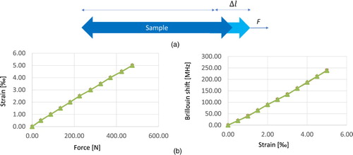
The strain is easily calculated using (13) ${\epsilon }_r=\frac{\Delta l}{l}\cdot 100[\mathrm{\%}]$(13) The measurements show that Brillouin sensitivity of the construction ranges from 476–480 MHz/% (Megahertz per-percent-strain) and the modulus of elasticity measured amounts to 4.48 GPa. The sensitivity of free optical fibre is ∼ 500 MHz/% and ∼ 1 MHz/°C for strain and temperature, respectively.

4.2. Cable bending measurements

The availability of more tightly buffered off-centered fibres inside the metal encapsulation gives possibilities for cable bending detection and measurements. The measurement principle is based on the fact that the cross-section above neutral axis is subjected to extension, and the cross-section below neutral axis is subjected to compression, whereas the central axis remains neutral and is not subjected to stress. The normal strain in the beam can be expressed as (14) $\epsilon =\frac{1}{\rho }z$(14) where $\rho$ is the curvature radius and $z$ is the distance from neutral axis. As the radius of curvature grows to infinity the normal strain decreases to zero. Figure 9 and Table 1 show real measurement curves and values of Brillouin peak shifts at the location 1031 m that was within observed bending segment.

Figure 9. Bending the sample with three fibres; (a) the configuration with dimensions and measurement results from all three fibres; fibre-1 (b), fibre-2 (c), fibre-3 (d); upper-right picture shows the Brillouin–Lorentzian profile (“the bell”) upper-left picture profiles the frequency shift of the peak across the length, bottom-left shows the gain and bottom right shows the width of Brillouin–Lorentzian profile.

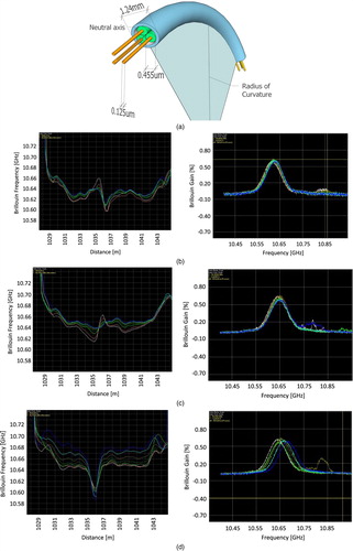
Table 1. Brillouin peak frequency shifts transition due to bending at the location 1031 m.

	Brillouin peak frequency shifts [GHz]
Brillouin Peak/Coil OD	OD 2000 mm	OD 1500 mm	OD 1000 mm	OD 500 mm	Slope Sign
Fiber1	10.6277	10.6252	10.6216	10.6154	Negative
Fiber2	10.6509	10.6478	10.6458	10.6409	Negative
Fiber3	10.6405	10.6465	10.6585	10.6840	Positive

Fibre-3 exhibits increase in Brillouin peak shift whereas the other two fibre nr. 1 and 2 exhibits decrease in Brillouin shift with stronger bending (Figure 10). This is the result of fibre 3 being in the extension zone above the neutral axis and the other two in compression zone.

Figure 10. Brillouin frequency peak shift with bending at position 1031 m.

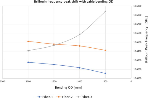
The careful analysis of magnitudes of the Brillouin peak shifts reveals information on the bending radius and applied tension in the segment that includes the bending and strain zone transition. This feature is due to multi-fibre configuration and can be exploited for development of measurement methods.

5. Conclusion

The cable with three tightly encapsulated optical fibres with OD 1.22 mm is nowadays producible in long lengths (15 km continuous length). Its linear strain characteristics is the reason for its adaptation and deployment into various geotechnical and geophysical commercial and scientific applications. Nevertheless, the potential goes much beyond strain measurements. The construction offers possibilities into pressure, bending and vibration detection and measurements and opens the way into more advanced versions able to discriminate the temperature from all other quantities. They are objectives of further research being conducted presently. Intrinsic multi-fibre design, innovative interrogation methods and algorithms and advanced optical fibre design together with precise production process will offer even more features to be realized in a small space. Therefore, it can be said, with confidence, that such a design will continue to be a valuable asset toward digitalization of energy cables, large structures and linear assets.

Disclosure statement

No potential conflict of interest was reported by the authors.

ORCID

Petar Bašić http://orcid.org/0000-0002-0882-4878

References

- Rogers A. Distributed optical-fibre sensing, Chapter 14. In: JM Lopez-Higuera, editor. Handbook of optical fibre sensing technology. New York, NY: John Wiley & Sons; 2002, p. 271–311.
- Horigushi T, Karashima T, Tateda M. A technique to measure distributed strain in optical fibers. IEEE Photonics Tchnol Lett. 1990;2:352. doi: 10.1109/68.54703
- Niklès M, Thévenaz L, Robert P. Simple distributed fiber sensor based on Brillouin gain spectrum analysis. Optics Lett. 1996;21(10):758. doi: 10.1364/OL.21.000758
- Cheng-Yu H, Yi-Fan Z, Guo-Wei L, et al. Recent progress of using brillouin distributed fiber sensors for geotechnical health monitoring. Sens Actuators. 2017.
- Bao X, Chen L. Recent progress in distributed fiber optic sensors. Sensors. 2012;12:8601–8639. doi: 10.3390/s120708601
- Patent application WO2014082965; Method for locally resolved pressure measurement.
- Rogers A. ‘Polarization in optical fibers’, Artech House Inc., ISBN-13: 978-1-58053-534-2, 2008.
- Rogers AJ.; ‘Polarization-optical time-domain reflectometry: a new technique for the measurement of field distributions’. Appl Opt 1981;20(6):1060–1074. doi: 10.1364/AO.20.001060
- Neil Ross J. Birefringence measurement in optical fibers by polarization-optical time-domain reflectometry. Appl Opt. October 1982;21(19):3489–3495. doi: 10.1364/AO.21.003489
- Niklès M, Thévenaz L, Fellay A, et al. “A novel surveillance system for installed fiber optics cables using Brillouin interaction”, Proceedings IWCS ‘97, p. 658–664.
- Niklès M, Thévenaz L, Salina P, et al. “Local analysis of stimulated Brillouin interaction in installed fiber optics cables”, OFMC ‘96, NIST Special Publication 905, p.111–114.
- Abaqus FEA simulation software, ABAQUS, Inc.
- Bašić P. “ Fiber optic sensors based on hollow capillary tube with three tightly encapsulated optical fibers”, PhD Thesis, University of Zagreb, Faculty of Electrical Engineering and Computing, 2019.
- Optical Time Domain Analysis (BOTDA) system – https://www.omnisens.com/index.html.
- Gogolla T, Krebber K. Distributed beat length measurementin single-mode optical fibers using stimulated brillouin-scattering and frequency-domain analysis. J Lightwave Technol. March 2000;18(3):320–328. doi: 10.1109/50.827503