Adaptive optimal slip ratio estimator for effective braking on a non-uniform condition road

ABSTRACT

In this paper, an adaptive algorithm is developed which senses the road condition change and estimates a (time-varying) optimal braking slip ratio. This is conducted by two on-line simultaneously operating tire-road friction-curve slope calculators: one based on the accelerometer output and the other based on the wheel speed. The required vehicle speed is estimated using a robust sliding-mode observer. Enforcement of the online optimal braking reference is left to an adaptive sliding mode controller to cope with the system strong nonlinearity, time dependency and the speed and friction-coefficient estimation errors. The algorithm is applied to a half model car and the braking performance is examined. The results indicate that the proposed algorithm substantially reduces the stopping time and distance. The performance of the algorithm is verified using different vehicle initial speeds and especially non-uniform road condition where 8% improvement versus the nonadaptive optimal slip ratio algorithm is recorded.

KEYWORDS:

• ABS
• adaptive sliding-mode control
• adaptive optimal slip ratio
• velocity observer

Nomenclatures

v	=	The vehicle speed
m	=	The vehicle mass
σ	=	The rolling resistance coefficient
σω	=	The tire viscous resistance coefficient
g	=	The gravity acceleration
J	=	The tire rotational inertia
R	=	The tire radius
µf(r)	=	The front (rear) tire-road friction coefficient
ωf(r)	=	The front (rear) tire angular velocity
df	=	The aerodynamic drag force coefficient
Fzf(r)	=	The front (rear) wheel normal force
Tbf(r)	=	The front (rear) braking torque
h	=	The height of the centre of gravity
Lf	=	The distance between the centre of gravity and the front axle
Lr	=	The distance between the centre of gravity and the rear axle
L	=	The distance between the front and the rear axle.
α	=	The vehicle actual acceleration.
v0	=	The maximum braking initial speed
λf(r)	=	The front (rear) tire slip ratio.
λo	=	The optimal slip ratio
ci(i = 1, 2, 3)	=	The road condition parameters
γ1, γ2	=	The relative upper bound of v and µ estimates.
D & H	=	The observer gain matrixes.

1. Introduction

Antilock braking system (ABS) ensures safe stopping by regulating the brake torques to provide maximum wheel traction force. This is conducted by estimating the optimal slip ratio, and enforcing it by a control technique. Thus, 3 algorithms are involved in an ABS: speed estimation, tire-road friction estimation, and control method.

The vehicle velocity cannot be measured directly due to the cost and technical issues. As a result, it may be estimated by an observer such as sliding mode [1–3], fusion Kalman/UFIR [4], and deadbeat dissipative FIR filtering [5].

Numerous parameters are involved in tire-road friction coefficients that are classified as vehicle parameters: speed, camber angle, and wheel load; tire parameters: material, tire type, tread depth, and inflation pressure; road lubricant parameters: water, snow, ice, oil, depth, and temperature; and road parameters: road type, micro-geometry, macro-geometry, and drainage capacity [6]. Generally speaking, the tire-road friction estimation methods are categorized under caused and effect-based approaches [7]. Cause-based approaches use special sensors like optical camera, infrared thermometers, temperature’ sensors and so on to detect road condition (water, snow, ice, oil, etc.) to be used later for friction estimation. In these methods, tire states (new or worn, winter tire or summer tire) or tire pressure are not taken into account. Alternatively, the effect-based approaches are at least classified into three types: acoustic, tire-tread deformation, and slip-based approaches [6].

In the slip- based approaches, the vehicle is commanded to follow the optimal slip ratio. The optimal slip ratio reflects the maximum tire-road friction coefficient, which directly manifests the road conditions. In [8], the recursive least-squares parameter identification method has been employed for tire-road friction coefficient estimation. The method uses a linear tire model and may become inaccurate when the slip ratio enters its nonlinear range. Estimation of the tire-road friction coefficient based on a combined APF-IEKF and iteration algorithm has been discussed in [9]. The tire-road friction parameter estimation using the extended Kalman filter is the subject of study in [1]. In [10] the tire forces are estimated by the discrete Kalman filter, and subsequently, the road friction coefficient is estimated by the recursive least square algorithm.

Control of uncertain systems requires a robust control technique such as fractional order PID [11], H_∞ [12,13] or sliding mode controllers [14–16]. Backstepping integral sliding mode controller is the subject of study in [17]. Adaptive SMC for control of ABS torque to secure optimal slip ratio following is presented in [1]. Employing backstepping control for ABS is the subject of study in [18]. Quasi-sliding mode Control along with the orthogonal endocrine Neural Network estimator for ABS control has been detailed in [19]. Using a multiple surface sliding controller for ABS has been dug out in [20]. In [21], a robust predictive control for ABS based on Radial Basis Function Neural Network has been proposed.

Regarding the above-mentioned developments in the ABS design where a constant offline computed optimal slip ratio reference is followed, in this paper, a road dependent online time-varying optimal slip ratio tracking scheme is adopted. The road condition dependent maximum brake traction force search is conducted using two measures, one based on the vehicle acceleration and another based on the wheel rotation speed. Besides the employed speed observer is designed in a way to overcome the wheel tachometer noise and the vehicle accelerometer offset. The braking discipline is enforced by an adaptive sliding mode controller to handle the system dynamic uncertainty and the estimators’ errors. As it is expected, the proposed ABS reduces substantially the braking stop time and the stopping distance due to the employment of the adaptive slip ratio estimator. This outstanding performance is verified by simulations considering various uniform and non-uniform road conditions and the vehicle initial speeds.

The paper is organized as follows: firstly, the system dynamic and the SMO speed estimation algorithm are detailed in Section 2. Online estimation of the optimal slip ratio is discussed in section 3. Section 4 covers the adaptive sliding mode control and lastly, the conclusion comes in Section 6.

2. Half Vehicle braking system model

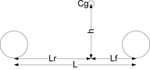
The half vehicle geometry that is used for the braking system study has been shown in Figure 1. The dynamic model of this system, based on Newton’s law of motion, is expressed by [1], (1) $\begin{array}{rl}m\dot{v}& =-{\mu }_f{F}_{zf}-{\mu }_r{F}_{zr}-\sigma mgv-d_f{v}^2\\ J{\dot{\omega }}_f& =R{\mu }_f{F}_{zf}+R\sigma F_{zf}v-{\sigma }_{\omega }{\omega }_f-T_{bf}\\ J{\dot{\omega }}_r& =R{\mu }_r{F}_{zr}+R\sigma F_{zr}v-{\sigma }_{\omega }{\omega }_r-T_{br}\end{array}$(1) By taking into account the front and rear tire normal forces, (2) $\begin{array}{rl}{F}_{zf}& =\frac{m\left(g{L}_r-h\dot{v}\right)}{L_f+L_r}=\frac{m\left(g{L}_r-ha\right)}{L}\\ F_{zr}& =\frac{m\left(g{L}_f+ha\right)}{L}\end{array}$(2)

Figure 1. The vehicle single-track geometric parameters.

Equation (1) is reformulated as below, (3) $\begin{array}{rl}\dot{v}& =\frac{-g({\mu }_f{L^{\mathrm{\prime }}}_r+{\mu }_r{L^{\mathrm{\prime }}}_f)-\sigma gv-d_f/m{v}^2}{1-h^{\mathrm{\prime }}\left({\mu }_f-{\mu }_r\right)}=a\\ {\dot{\omega }}_f& =J^{-1}\left(mgR\sigma {L^{\mathrm{\prime }}}_{r}v-{\sigma }_{\omega }{\omega }_f-T_{bf}-f_f\right)\\ {\dot{\omega }}_r& =J^{-1}\left(mgR\sigma {L^{\mathrm{\prime }}}_{f}v-{\sigma }_{\omega }{\omega }_r-T_{br}+f_r\right)\end{array}$(3) where (4) $\begin{array}{rl}{f}_f& =mR\left[\frac{g{\mu }_f(h^{\mathrm{\prime }}{\mu }_r+L{}_r^{\mathrm{\prime }}+{\sigma }_v{h}^{\mathrm{\prime }}v)}{h^{\mathrm{\prime }}({\mu }_f-{\mu }_r)-1}+h^{\mathrm{\prime }}{\sigma }_{v}a\right]\\ f_r& =mR\left[\frac{g{\mu }_r(h^{\mathrm{\prime }}{\mu }_f+L{}_f^{\mathrm{\prime }}+{\sigma }_v{h}^{\mathrm{\prime }}v)}{h^{\mathrm{\prime }}({\mu }_f-{\mu }_r)-1}+h^{\mathrm{\prime }}{\sigma }_{v}a\right]\\ L{}_f^{\mathrm{\prime }}& =\frac{L{}_f^{\mathrm{\prime }}}{L},L{}_r^{\mathrm{\prime }}=\frac{L_r}{L},h^{\mathrm{\prime }}=\frac{h}{L}\end{array}$(4) Now, the state space representation of (3) is expressed by the following equation, (5) $\begin{array}{rl}\dot{x}& =Ax+Bu+f_n\\ y& =Cx\\ \dot{x}& =\frac{1}{J}\left[\begin{array}{ccc}0& 0& 0\\ mgR\sigma L{}_r^{\mathrm{\prime }}& -{\sigma }_{\omega }& 0\\ mgR\sigma L{}_f^{\mathrm{\prime }}& 0& -{\sigma }_{\omega }\end{array}\right]x\\ & +\frac{1}{J}\left[\begin{array}{ccc}0& 0& 0\\ 0& 1& 0\\ 0& 0& 1\end{array}\right]\left[\begin{array}{c}0\\ T_{bf}\\ T_{br}\end{array}\right]+\frac{1}{j}\left[\begin{array}{c}a\\ -f_f\\ f_r\end{array}\right]\\ y& =\left[\begin{array}{ccc}0& 1& 0\\ 0& 0& 1\end{array}\right]x\end{array}$(5) where x = [v, ω_f, ω_r]^T, y = [ω_f, ω_r], and α are the state variable, the measured output, and the vehicle actual acceleration, respectively.

2.1. The vehicle velocity observer

For the computation of the optimal slip ratio, the vehicle speed is required. It may be measured or estimated. For the estimation of the vehicle speed, the following sliding mode observer using (5) is formed [22], (6) $\begin{array}{rl}& \hat{\dot{x}}=A\hat{x}+Bu+D.C.e+H.\mathrm{sgn}\left(Ce\right)\\ & y-\hat{y}=Ce=C(x-\hat{x})\end{array}$(6) where (A, C) must be observable and D and H are both 3 by 2 observer gain matrixes. Using (5) and (6), the state estimation error is obtained as given below, (7) $\dot{e}=(A-DC)e+f_n-H.\mathrm{sgn}\left(Ce\right)$(7)

To design a stable observer, it is analyzed using V = e^Te/2 Lyapunov function as pursued in below, (8) $\begin{array}{rl}\dot{V}& =-e_1\left(h_{{}_{11}}\mathrm{sgn}\right(e_2)+h_{{}_{12}}\mathrm{sgn}(e_3)-a)\\ & +\left(\frac{mgR\sigma {L^{\mathrm{\prime }}}_r}{J}-d_{11}\right)e_1{e}_2\\ & +\left(\frac{mgR\sigma {L^{\mathrm{\prime }}}_f}{J}-d_{12}\right)e_1{e}_3-\left(h_{21}-h_{22}-\frac{|f_f|}{J}\right)|e_2|\\ & -\left(h_{32}-h_{31}-\frac{|f_r|}{J}\right)|e_3|-\frac{d_{22}+d_{31}}{2}(e_2+e_3{)}^2\\ & -\left(\frac{\sigma }{J}+d_{21}-\frac{d_{22}+d_{31}}{2}\right)e_2^2\\ & -\left(\frac{\sigma }{J}+d_{32}-\frac{d_{22}+d_{31}}{2}\right)e_3^2\end{array}$(8) Considering (8), the observer asymptotic stability is met if the following conditions are observed, (9) $\begin{array}{rl}{d}_{11}& =\frac{mgR\sigma L{}_r^{\mathrm{\prime }}}{J}{d}_{12}=\frac{mgR\sigma L{}_f^{\mathrm{\prime }}}{J}\\ & d_{22}+d_{31}=\beta \ge 0\\ & h_{21}>\frac{|f_f|}{J}{h}_{32}>\frac{|f_r|}{J}{h}_{12}=\alpha .sgn\left(e_3\right)\\ d_{21}& =d_{32}>\frac{\beta }{2}\end{array}$(9) where the rest of the elements of C and D matrices are zero. d₁₁, d_22, and h₁₂ are computed using the system available parameters and variables. d₁₁, d₃₁, d_21, and d₃₂ are calculated by taking a relatively large value for β, which improves the estimation speed. h₂₁ and h₃₂ are determined using (4) based on the known system parameters and the design assumptions for the maximum braking initial speed, v_0, and its subsequent deceleration, max(|α|). Since the braking system operates in a closed loop form; both λ_r and λ_f are forced to follow a single λ_o, therefore, it is reasonable to assume an almost equal friction coefficient for the front and rear wheels. Thus, while the exact values for f_f and f_r (9) are not available, those can be estimated using $\dot{\hat{x}}$ (1) and the estimated speed $\hat{v}$ becomes, (10) $\hat{\mu }={\mu }_f\simeq {\mu }_r=\frac{-\hat{\dot{x}}\left(1\right)}{g}-\sigma \hat{v}-\beta {\hat{v}}^2\beta =\frac{d_f}{gm}$(10) The observability condition of the SMO is impaired in case of small values of the rolling resistance coefficient, σ, where the observer estimation performance is degraded. By choosing big h₂₁, h₃₂, the SMO gets robust to the system parameter variations. In the case of partial known f_n, the known part is employed in (9).

3. On-line estimation of the optimal slip ratio

The tire-road friction is a function of the tire slip ratio and the road conditions as it is shown in Figure 2. By the increase in the slip ratio, the friction coefficient arises sharply until it touches its peak and then falls slowly. Thus, there is a maximum friction coefficient for each road condition; therefore, the optimal slip ratio, which reflects this peak is a function of the road condition.

Figure 2. The variation of the friction coefficient, µ against the slip ratio, λ on different road conditions [1].

One of the models for the tire-road friction coefficient is the Burckhardt tire model [23] which is expressed by the following equation, (11) $\mu \left(\lambda \right)=c_1[1-\exp (-c_2\lambda \left)\right]-c_3\lambda$(11) where c_i(i = 1, 2, 3) reflect the road conditions. The data for some typical road conditions have been given in Table 1.

Table 1. Constants for different road conditions [24].

Road surface	c1	c2	c3
Dry asphalt	1.28	23.99	0.52
Wet asphalt	0.857	33.82	0.34
Snow	0.194	94.12	0.0646
Ice	0.05	306	0

3.1. Tire-road friction peak detection

The braking process is divided into three phases, pre-braking, braking inception, and optimal braking. In the pre braking interval where no brake and or acceleration forces are applied, λ is almost zero and the model parameters σ and d can be estimated using the available acceleration, α, and the estimated speed $\hat{v}$ = Rω_f. 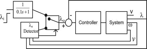This is conducted by utilizing the least squares algorithm, which is applied to the following linear regression model extracted from (1), (12) $\dot{v}=-\left[\sigma d/m\right]\left[\begin{array}{c}\hat{v}\\ {\hat{v}}^2\end{array}\right]=a$(12) In order to estimate the peak of the tire-road friction, during the braking inception phase, a step λ_r is applied to the ABS through a time constant with a value beyond the friction coefficient peak for any road condition, namely λ_i = 0.4. Then µ is monitored using (10) by the peak detector block, shown in Figure 3. As soon as it reaches its peak, the block switches the slip ratio to the captured newly optimal level and the control proceeds.

Figure 3. The ABS control system.

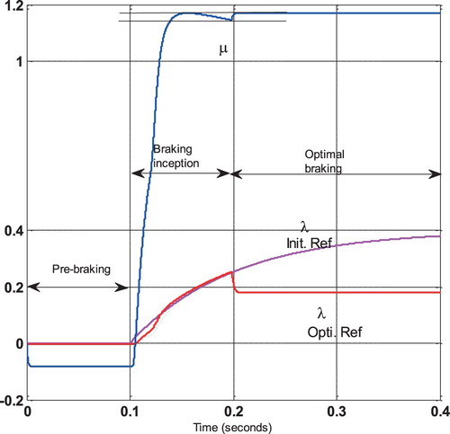
The operation in each phase has been portrayed in Figure 4. The initial reference and the computed optimal slip ratio have been shown. By following the optimal reference, the traction force rolls back again to its maximum value. Obviously, the detected level is a function of the road condition.

Figure 4. The braking timing.

Subsequently, for the algorithm to cope with the change in the road condition during braking, an on-line recursive optimal slip ratio procedure is incorporated as given below, (13) $\begin{array}{rl}{\lambda }_o\left(k\right)& ={\lambda }_o(k-1)+\mathrm{0.01.}\text{sign}\left({\mathrm{\Delta }}_{\mu }\right)\\ {\mathrm{\Delta }}_{\mu }& =\hat{\mu }(k-1)-\hat{\mu }(k-2)\end{array}$(13) where µ is given by (10). Since in the steady state, the closed-loop control system forces $\dot{\lambda }$ to zero; it prevents the computation of $\dot{\mu }$ = Δ_µ, the peak search direction. Fortunately, the friction curve (11) is unimodal and the sign if Δµ is sufficient for the friction curve slope determination as it has been emplaced in (13).

While the above scenario may fail in a real application due to road nonuniformities and accelerometer error, the slope is double checked using equations based on the wheel rotation speed to accompany the slope detector given in (13). Friction curve slope detection using wheel speed rotation has already been experimentally tested in [25]. Detection of the friction curve slope is pursued, here, differently from [25], where the wheel rotation speed of the rear and front wheels (1) are added together to discard the direct effect of the vehicle acceleration. Alternatively, the following second equation for µ is developed, (14) $\begin{array}{rl}Rmg{\mu }_{\omega }& =J\underset{\_}{\dot{\omega }}-R\sigma mgv+{\sigma }_{\omega }\underset{\_}{\omega }+{\underset{\_}{T}}_b\Rightarrow \\ \text{sign}\left({\mathrm{\Delta }}_{\mu }\right)& =\text{sign}\left(\mathrm{\Delta }(J\underset{\_}{\dot{\omega }}-R\sigma mgv+{\sigma }_{\omega }\underset{\_}{\omega }+{\underset{\_}{T}}_b)\right)\end{array}$(14) where the underlined, ω and T_b variables are the summation of the corresponding rear and front wheel variables.

4. ABS adaptive sliding mode control

Should the optimal slip ratio λ_o is available, the vehicle ABS performance is maintained where the ABS control loop accurately sticks to the given λ_o by adjusting the braking torques. However, due to the strong nonlinear, time variant and uncertain nature of the braking process, robust control methods such as sliding mode control is requisite for the successful conduction of the task.

To implement SMC for the front wheel, based on the front tire slip ratio tracking error, the following standard sliding-mode surface is defined, (15) $e_f={\lambda }_f-{\lambda }_{fo}\Rightarrow s_f=e_f+k_{1f}{\int }_0^t{e}_f\left(\tau \right)\text{d}\tau$(15) where k_1f is the front tire sliding-mode positive constant factor to be appropriately assigned. It affects the transient response of the control system. By making the derivative of the sliding surface zero, the following relation is attained, (16) ${\dot{s}}_f={\dot{\lambda }}_f-{\dot{\lambda }}_{fo}+k_{1f}{e}_f=0\Rightarrow {\dot{\lambda }}_f={\dot{\lambda }}_{fo}-k_{1f}{e}_f$(16)

By utilizing (3), the change in the slip ratio is obtained in compact form as below, (17) ${\dot{\lambda }}_f=g_f+b_f{T}_{bf}$(17) where (18) $\begin{array}{rl}{g}_f& =\frac{{\omega }_{f}Ra}{v^2}+\frac{f_f-\frac{mgR\sigma L_{r}v}{L}+{\sigma }_{\omega }{\omega }_{f}R}{Jv}\\ b_f& =\frac{R}{Jv}\end{array}$(18)

Substituting (17) in (16) gives, (19) ${\dot{s}}_f=g_f+b_f{T}_{bf}-{\dot{\lambda }}_{fo}+k_{1f}{e}_f$(19) Assuming the nominal system, the tracking error converges to zero using the following continuous command, (20) $T_{bf}=-b_f^{-1}\left(g_f-{\dot{\lambda }}_{fo}+k_{1f}{e}_f\right)$(20)

However, for the exact system, the control objective may no longer be satisfied and an additional switching control is required to take care of the uncertainty damaging effect. Thus, Equation (20) is replaced with the following equation, (21) $T_{bf}=-{\hat{b}}_f^{-1}\left({\hat{g}}_f-{\dot{\lambda }}_{fo}+k_{1f}{e}_f+k_{2f}{\tan }^{-1}\left(s_f\right)\right)$(21) where $\hat{b}$ has been used due to the employment of the estimated velocity.

To analyze the closed loop ABS stability, $s_f^2/2$ Lyapunov function is investigated. It is straightforward and procedural [1] to reach a result for the switching gain k_2f that enforces the asymptotic stability. The adaptive gain is concluded as [1], (22) $\begin{array}{rl}{k}_{2f}& =\frac{{\gamma }_1\left(2+{\gamma }_1\right){\omega }_{f}R.a}{{\left(1-{\gamma }_1\right)}^2{\hat{v}}^2}+\frac{R{A}_f}{J}+\frac{R}{J}\left|\frac{{\hat{f}}_f}{\hat{v}}\right|\\ & +\frac{{\gamma }_1}{\left(1-{\gamma }_1\right)}\frac{{\sigma }_{\omega }{\omega }_{f}R+R{T}_{bf}}{J\hat{v}}\end{array}$(22) where (23) $\begin{array}{rl}{A}_f& =\frac{mgR}{1+2{\gamma }_{2}h\hat{\mu }}\left(\phantom{\frac{\left(1+{\gamma }_2\right)\hat{\mu }h+L_r+h\sigma )}{\left(1-{\gamma }_1\right)\hat{v}}}h{\sigma }^2+\left(1+{\gamma }_2\right)\hat{\mu }\left(\phantom{\frac{\left(1+{\gamma }_2\right)\hat{\mu }h+L_r+h\sigma )}{\left(1-{\gamma }_1\right)\hat{v}}}h\sigma \right.\right.\\ & \left.\left.+\frac{\left(1+{\gamma }_2\right)\hat{\mu }h+L_r+h\sigma )}{\left(1-{\gamma }_1\right)\hat{v}}\right)\right)\end{array}$(23)

γ₁ and γ₂ are the relative upper bound of the estimated speed and µ’s, respectively.

Similarly, the same can be repeated for the rear wheel that renders the following results [1], (24) $\begin{array}{rl}{k}_{2r}& =k_{2(f\to r)}\\ A_r& =\frac{mgR}{1+2{\gamma }_{2}h\hat{\mu }}\left(\phantom{\frac{\left(1+{\gamma }_2\right)\hat{\mu }h-L_f+h\sigma )}{\left(1-{\gamma }_1\right)\hat{v}}}h{\sigma }^2+\left(1+{\gamma }_2\right)\hat{\mu }\left(\phantom{\frac{\left(1+{\gamma }_2\right)\hat{\mu }h-L_f+h\sigma )}{\left(1-{\gamma }_1\right)\hat{v}}}h\sigma \right.\right.\\ & \left.\left.+\frac{\left(1+{\gamma }_2\right)\hat{\mu }h-L_f+h\sigma )}{\left(1-{\gamma }_1\right)\hat{v}}\right)\right)\end{array}$(24)

5. Simulations

In order to validate the performance of the designed ABS system, several tests are conducted. The vehicle specifications have been depicted in Table 2. The simulations are performed using SIMULINK.

Table 2. Tyre and vehicle parameters [1].

Pars	Values	Pars	Values
v0	20 m/s	h	0.5 m
m	2045 kg	Lf	1.488 m
R	0.3 m	Lr	1.712 m
J	1.5 kgm^2	σ	1
L	3.2 m	df	0.45
		σω	0.005

In order to check the controller performance alone in tracking the issued slip ratio command, a first test is conducted. The speed is assumed measured and the road condition is uniform dry asphalt introduced by c₁ = 1.28, c₂ = 23.99, and c₃ = 0.52 parameters. The step λ_i = 0.4 is applied to the designed ABS. The system behaviour is shown in Figure 5.

Figure 5. The ABS controller performance in tracking the issued arbitrary slip ratio command.

The braking lasts for 1.807s corresponding to 18.92 m stopping distance. As the figure indicates, in some instances the vehicle experiences a higher friction coefficient than the other times. It is desirable that the peak of the traction force is employed during the entire optimal braking phase (phase 3). The (reference) slip ratio tracking performance of the controller is visualized from the rear and front wheels slip ratio variable curves, where zero steady-state error and good transient response have been registered in Figure 5.

To show, how assigning optimal level for the slip ratio improves the stopping performance; the µ peak- detector algorithm is put into operation. Again, the vehicle speed is assumed measured and uniform dry asphalt road condition is preserved. During this test, the braking time and the stopping distance are 1.674 s and 17.61 m, respectively. There is around a 1.3 m reduction in the braking distance. The results have been depicted in Figure 6. Thus, around 7% shorter stopping distance is obtained when the optimal slip ratio is impelled.

Figure 6. The ABS performance using µ peak detector and the optimal slip ratio reference.

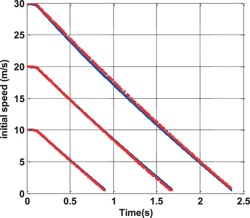
As it is mentioned earlier, often vehicles are not equipped with a direct speed sensor; rather the speed is estimated based on the vehicle acceleration and the wheel rotational speed. The variance of the $\omega$ sensors noise is assigned 0.1 and the accelerator sensor offset is set 0.3. The estimator parameters are set as given in (9) and d21 = d32 = 100. The performance of SMO in the estimation of the vehicle speed under various speed initial conditions has been portrayed in Figure 7. The speed estimation absolute error is almost less than 0.5 m/s constant. As a result, the relative error at speeds above 5 m/s is below 10% and at the end of the stopping stage at 2.5 m/s speed, it may reach 20%. Thus, it looks sufficient to consider 20% tolerance (γ₁ = 0.2) for the estimated speed.

Figure 7. The performance of the speed estimator under various initial braking speed.

The tolerance in the estimation of v affects the µ estimation expressed by (10). From analyzing (10) with the parameters given in Table 2, it is realized that 20% tolerance in the velocity has less than 5% (γ₂ = 0.05) effect on the estimation of µ. Thus, γ₁ = 0.2 and γ₂ = 0.05 uncertainty bound are emplaced in the ASMC command (22) to deliver a robust behaviour. Testing the designed ABS performance using the estimated speed has been shown in Figure 8. The traction force peak detector marks the peak and the SMC forces the rear and the front wheel slip ratio to pursue the derived optimal slip ratio. In this test, the stopping time of 1.687 s and the stopping distance of 17.87 m are recorded.

Figure 8. The performance of the ABS adaptive sliding mode control using $\hat{v}$.

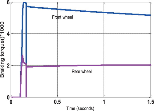
While the controller manages the braking based on the estimate of the vehicle speed, still the steady state tracking error is zero, indicating excellent SMC robustness in performance. The transient behaviour of the controller has also been shown in Figure 8, where appropriate reference following has been recorded. The corresponding braking force curves have been depicted in Figure 9 where not much disturbing switching is observed. Despite uniform road condition, different brake force for the rear and the front wheel has been applied due to the different wheel normal forces.

Figure 9. The rear and front wheels braking torques.

The ABS performance on a wet asphalt road with the c₁ = 0.857, c₂ = 33.82, and c₃ = 0.34 parameters delivers 2.548 s stopping time corresponding to the 25.9 m stopping distance. Comparing with the dry asphalt test, 0.861 s higher braking time and 8.03 m larger stopping distance is obtained.

5.1. Effective braking over a non-uniform condition road

In order to investigate the effectiveness of the proposed ABS strategy on a non-uniform road condition, it is assumed that the braking is started on the dry asphalt at t = 0 sec and at time t = 1 s the road condition turns to the wet asphalt. Figure 10 shows how this affects the speed estimation process. In spite of the changes in the road condition, an acceptable estimation of the speed is obtained and the actual and the estimated velocities are almost laid on each other.

Figure 10. The vehicle speed and its estimation over a non-uniform condition road.

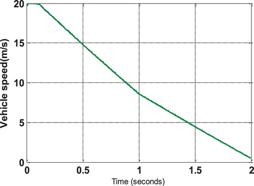
The braking time of 2 s and the stopping distance of 19.28 m is achieved if no online update of the optimal breaking is performed. However, with the conduction of the online road condition monitoring the response changes and the stopping time drops to 1.974 s and the stopping distance reduces to around 18.93 m. The slope detector algorithm enjoys the association of the following two slope detector equations; to prevent the generation of any wrong or noisy slip ratio reference, (25) $\begin{array}{rl}\text{sign}\left(\mathrm{\Delta }\mu \right)& =\text{sign}\left(\mathrm{\Delta }\right(-a-0.05\hat{v}-0.3\ast {10}^{-4}{\hat{v}}^2\left)\right)\\ \text{sign}\left(\mathrm{\Delta }\mu \right)& =\text{sign}\left(\mathrm{\Delta }\right(1.2\dot{\omega }-30\hat{v}+\omega +T_b\left)\right)\end{array}$(25) 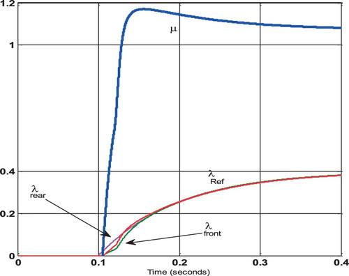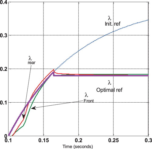where the top equation is based on the change in the acceleration and the second one relys on the rotational wheel speed. The system response has been depicted in Figure 11 where the traction force coefficient, optimal slip ratio reference and the actual front and rear wheel slip ratios are exhibited. The change in the slip ratio toward its optimal value at t = 1 sec has been zoomed to better illustrate the controller performance. Utilizing the optimal ABS delivers (2−1.974 = 0.026 s) drop in the braking interval and (19.28−18.93 = 0.35 m) reduction in the stopping distance in this test.

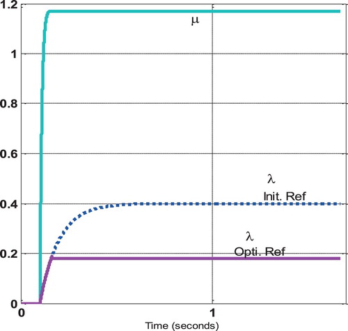
Figure 11. Effective braking on a nonuniform road condition; the varying optimal reference slip ratio reference (λ) and the maximum attainable tire-road friction coefficient (µ).

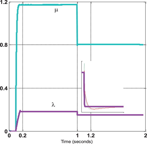
This means that using the proposed adaptive optimal slip ratio estimator has reduced the barking distance by around 8%, which makes it a promising strategy to be embedded in the new anti-lock braking systems. Such an algorithm could serve greatly in preventing financial costs and human casualties. The summary of the conducted tests has been presented in Table 3. The dry, wet and dry/wet asphalt conditions for the road, the measured and the estimated values for the speed, and the fixed, optimal and adaptive optimal values for the slip ratio cases are provided for comparison of the results. The last two rows of the table compare the result of the algorithm in [1] with the currently proposed algorithm.

Table 3. Summary of several conducted tests.

	Speed value		Slip ratio (λ) value			Braking performance
Asphalt condition	Measured	Estimated	Fixed (=0.4)	Optimal	Adaptive optimal	Time (s)	Distance (m)
Dry	*	–	*	–	–	1.807	18.92
Dry	*	–	–	*	–	1.674	17.61
Dry	–	*	–	*	–	1.687	17.87
Wet	–	*	–	*	–	2.548	25.9
DWP^a [1]	–	*	–	*	–	2	19.28
DWP^a	–	*	–		*	1.974	18.93

^aDry & Wet patches.

6. Conclusion

The antilock braking system is under great scrutiny, as vehicle safety is highly desired. The centre core of the proposed ABS system is an adaptive optimal slip ratio tracker, which examines changes in the road condition in the braking phase. The algorithm detects the friction curve peak using a fusion of the output of two algorithms; one based on the vehicle acceleration and another based on the wheel rotation speed. The required vehicle speed estimation is managed by an adaptive sliding mode observer, which is capable of suppressing the measurement noise and sensor offset. Enforcement of the control objective is also conducted using a robust adaptive sliding mode controller to contain the system dynamic uncertainty and disturbances. As a result, an ABS is formed that delivers efficient braking by reducing the braking time and stopping distance. The online tire-road coefficient estimator makes the method right for the optimum and effective braking on a non-uniform road condition; where 8% in the stopping distance reduction is obtained using adaptive road condition dependent optimal λ_o versus constant optimal λ_o. The findings are verified through extensive simulations, which confirm the promising potential of the method.

Acknowledgment

This work has been partially supported by the research department of Shahed University, Tehran, IRAN.

Disclosure statement

No potential conflict of interest was reported by the authors.

ORCID

S. Seyedtabaii http://orcid.org/0000-0001-7617-5542

References

- Zhang X, Yong X, Ming P, et al. A vehicle ABS adaptive sliding-mode control algorithm based on the vehicle velocity estimation and tyre/road friction coefficient estimations. Veh Syst Dyn. 2014;52(4):475–503. doi: 10.1080/00423114.2013.864775
- Rascón R. Robust tracking control for a class of uncertain mechanical systems. Automatika. 2019;60(2):124–134. doi: 10.1080/00051144.2019.1584693
- Nemati M, Seyedtabaii S. Fault severity estimation in a vehicle cooling system. Asian J Control. 2019:1–6. DOI:10.1002/asjc.2155.
- Zhao S, Shmaliy YS, Shi P, et al. Fusion Kalman/UFIR filter for state estimation with uncertain parameters and noise statistics. IEEE Trans Ind Electron. 2017;64(4):3075–3083. doi: 10.1109/TIE.2016.2636814
- Ahn CK, Shi P, Basin MV. Deadbeat dissipative FIR filtering. IEEE Trans. on Circuits and Systems. 2016;63(8):1210–1221. doi: 10.1109/TCSI.2016.2573281
- Uchanski M, Hedrick K. Estimation of the maximum tire-road friction coefficient. J Dyn Syst Meas Control. 2003;125(12):607–617.
- Zhang X, Göhlich D. A hierarchical estimator development for estimation of tire-road friction coefficient. PLoS one. 2017;12(2):e0171085. doi: 10.1371/journal.pone.0171085
- Rajamani R, Phanomchoeng G, Piyabongkarn D, et al. Algorithms for real-time estimation of individual wheel tire-road friction coefficients. IEEE/ASME Trans Mechatron. 2012;17(6):1183–1195. doi: 10.1109/TMECH.2011.2159240
- Liu Y-H, Li T, Yang Y-Y, et al. Estimation of tire-road friction coefficient based on combined APF-IEKF and iteration algorithm. Mech Syst Signal Process. 2017;88:25–35. doi: 10.1016/j.ymssp.2016.07.024
- Zhao J, Zhang J, Zhu B. Development and verification of the tire/road friction estimation algorithm for antilock braking system. Math Probl Eng. 2014;2014:1–15. DOI:10.1155/2014/786492.
- Seyedtabaii S. New flat phase margin fractional order PID design: Perturbed UAV roll control study. Rob Auton Syst. 2017;96:58–64. doi: 10.1016/j.robot.2017.07.003
- Seyedtabaii S, Zaker S. Lateral control of an Aerosonde facing tolerance in parameters and operation speed: performance robustness study. Trans Inst Meas Control. 2019;41:2319–2327. doi: 10.1177/0142331218799142
- Seyedtabaii S. A modified FOPID versus H∞ and µ synthesis controllers: robustness study. Int J Control, Autom Syst. 2019;17(3):639–646. doi: 10.1007/s12555-018-0033-x
- Seyedtabaii S, Delavari M. The choice of sliding surface for robust roll control: Better suppression of high angle of attack/sideslip perturbations. Int J Micro Air Vehicles. 201810:330–339. doi: 10.1177/1756829318771059
- Hosseini M, Seyedtabaii S. Robust ROV path following considering disturbance and measurement error using data fusion. Appl Ocean Res. 2016;54:67–72. doi: 10.1016/j.apor.2015.10.009
- Rezaee M, Seyedtabaii S. On an optimized fuzzy supervized multiphase guidance law. Asian J Control. 2016;18(6):2010–2017. doi: 10.1002/asjc.1283
- Coban R. Backstepping integral sliding mode control of an electromechanical system. Automatika: časopis za automatiku, mjerenje, elektroniku, računarstvo i komunikacije. 2018;58(3):266–272. doi: 10.1080/00051144.2018.1426263
- Patil A, Ginoya D, Shendge P, et al. Uncertainty-estimation-based approach to antilock braking systems. IEEE Trans Veh Technol. 2016;65(3):1171–1185. doi: 10.1109/TVT.2015.2413451
- Perić SL, Antić DS, Milovanović MB, et al. Quasi-sliding mode control with orthogonal endocrine neural network-based estimator applied in anti-lock braking system. IEEE/ASME Trans Mechatron. 2016;21(2):754–764. doi: 10.1109/TMECH.2015.2492682
- Verma R, Ginoya D, Shendge P, et al. Slip regulation for anti-lock braking systems using multiple surface sliding controller combined with inertial delay control. Veh Syst Dyn. 2015;53(8):1150–1171. doi: 10.1080/00423114.2015.1026831
- Mirzaeinejad H. Robust predictive control of wheel slip in antilock braking systems based on radial basis function neural network. Appl Soft Comput. 2018;70:318–329. doi: 10.1016/j.asoc.2018.05.043
- Zhang J, Swain AK, Nguang SK. Robust sliding mode observer based fault estimation for certain class of uncertain nonlinear systems. Asian J Control. 2015;17(4):1296–1309. doi: 10.1002/asjc.987
- Burckhardt M. Fahrwerktechnik: Radschlupf-regelsysteme. Wrzburg: Vogel Verlag; 1993.
- Sardarmehni T, Rahmani H, Menhaj MB. Robust control of wheel slip in anti-lock brake system of automobiles. Nonlinear Dyn. 2014;76(1):125–138. doi: 10.1007/s11071-013-1115-1
- Tanelli M, Savaresi SM. Friction-curve peak detection by wheel-deceleration measurements. IEEE Intelligent Transportation Systems Conference; 2006 Sep. IEEE; 2006. p. 1592–1597.