Research and implementation of parallel artificial bee colony algorithm based on ternary optical computer

Abstract

The artificial bee colony (ABC) algorithm is a widely used algorithm in the field of function optimization problems. The traditional ABC algorithm has long search time, slow convergence speed and easy to fall into local optimum at the end of the search. In this paper, the design scheme and method of implementing parallel ABC algorithm are studied, which makes use of the characteristics of many data bits and easy expansion of data bits of the ternary optical computer (TOC). First, by analysing the traditional ABC algorithm, we can find the parallel parts and parallel design. Then the detailed algorithm implementation flow is given and the clock cycle of the algorithm is analysed. Finally, the correctness of the parallel scheme is verified by experiments. Compared with the ABC algorithm and parallel ABC algorithms based on computer (PABC), the ABC algorithm based on TOC (TOC-PABC) effectively shortens the search time, improves the optimization performance of complex multimodal function optimization problems and obtains a higher speedup.

KEYWORDS:

• Ternary optical computer
• parallel computing
• swarm intelligence
• artificial bee colony algorithm

1. Introduction

In 2005, Karaboga proposed an artificial bee colony (ABC) algorithm based on Seeley's colony self-organizing model [1]. The algorithm is a swarm intelligence optimization algorithm for simulating honey bee collecting behaviour and achieves target search through bee colony division of labour. It has the characteristics of simple parameter setting and easy implementation. The algorithm can solve a series of optimization problems, including function optimization and combinatorial optimization problem [2–4], etc. Literature [5–6] improved the ABC algorithm and improved the search performance to some extent. In the literature [7], an improved artificial bee colony algorithm (IABC) is proposed, which uses the generation of adjacent solutions to improve the ABC algorithm. Aiming at the drawback of ABC algorithm with local search ability, the literature [8] proposed an ABC algorithm based on the balanced search. However, many of the existing ABC algorithms are serial. When solving large-scale complex engineering optimization problems, the search performance of serial ABC algorithm is not ideal. This poses a challenge to the traditional ABC algorithm in finding the optimal solution of the function, so it is necessary to seek new solutions to meet this challenge.

The ternary optical computer (TOC) is named after its processor uses three-state optical signals to represent information and can perform all ternary logic operations [9]. The biggest difference between this optical processor and the traditional electronic processor is that optical processor allows the user to reconfigure the calculation function of each data bit at any time, and a large number of data bits can be grouped arbitrarily [10]. These advantages make it more suitable to solve the problems faced by the current ABC algorithm. TOC uses liquid crystal arrays and embedded control components, so compared with electronic computers, TOC's lower energy consumption, less heat, and its numerous data bits and data bits are easy to expand, making it more suitable for parallel implementation of ABC algorithm in hardware. At present, TOC has a preliminary theoretical system and experimental platform [11–16]. Beginning with the idea of publishing TOC in 2003, after Decrease-Radix Design theory [17], TOC encoder and decoder [18], FFT algorithm implementation and DFT algorithm implementation [19,20], performance analysis of a TOC [21], improved symbol number (MSD) adder [22–26], the implementation of reconfigurable ternary optical processor [27,28] and vector matrix multiplication [29,30], cellular automata [31] and other TOC-based applications, the current TOC has the conditions to implement parallel ABC algorithm.

This paper makes use of the advantages of TOC data bits and can be reconstructed at any time. By decomposing the parallel part of ABC algorithm in the search process, ABC algorithm can realize parallel search on hardware, thus improving search speed and optimization performance as a whole. And introduces the characteristics of TOC and the corresponding addition and multiplication operations, analyses the parallelism of ABC algorithm, and the implementation scheme on TOC, and analyses the clock cycle in the implementation process.

2. Related work

2.1. ABC algorithm

In ABC algorithm, the position of the food source refers to a feasible solution in the optimization problem, and the richness of the food source indicates whether the quality (fitness value) of the solution is high. The ABC algorithm consists of employed bees, onlooker bees and scout bees. Generally, the number of employed bees and onlooker bees is equal, and the number of scout bees is 1. In the ABC algorithm, the process of collecting honey of employed bees is similar to the process of finding the optimal solution in evolutionary computation. The honey source of the bee search is expressed as a possible solution. The whole process of searching for the honey source is equivalent to searching for the optimal solution. The quality of the honey source is regarded as the fitness value fit. The corresponding relationship between bee collecting honey and optimization problems is shown in Table 1.

Table 1. Corresponding relationship between bee collecting honey and optimization problems.

Bee collecting honey	Optimization problems
Honey source location	Feasible solution
Quality of honey source	Quality of feasible solution
Speed of collecting honey	Optimized speed of feasible solution
Maximum fit value	Optimal solution

In the ABC algorithm, the behaviour of collecting honey contains three main factors: food source, employed bees and unemployed bees.

1. Food source. Food source refers to various possible solutions. The quality of food depends on many factors, such as the distance from the hive, the concentration of honey source, whether it is easy to be extracted, etc., which is attributed to fitness.

2. Employed bees. The employed bees are associated with food sources that carry information about specific food sources, including the distance of the food source from the hive, the direction of the food source and the quality. The employed bees share this information with other bees by jumping and dancing.

3. Unemployed bees are divided into two types: onlooker bees and scout bees, and the scout bees are responsible for searching for food sources near the hive. The onlooker bees wait in the hive, looking for the employed bees to follow by observing the dance of the employed bees. Once the employed bees are selected to be followed, the onlooker bees become the employed bees.

The group of solutions is represented by SN D-dimensional vectors. The ith solution can be expressed as x_i, x_i= (x_i1, x_i2, … , x_iD), i = 1, 2, … , SN. The amount of pollen from the food source corresponds to the quality of the solution. Fitness is represented by fit₁, fit₂, … , fit_SN. If a food source has not been updated after a preset maximum number of cycles limit, then the employed bee will give up the food source to become a scout bee. The basic principles can be described as follows:

(1) Initialize the food source

In the initial state of the ABC algorithm, the scout bees search for SN food sources randomly. Generated according to Equation (1): (1) $x_{ij}=x_{\text{min}}(j)+\text{rand}(0,1)\cdot (x_{\text{max}}(j)-x_{\text{min}}(j))$(1) where x_ij is the j-dimensional coordinate of the food source x_i and x_max(j), x_min(j) are the two boundary values of the search space, and rand is a random number between 0 and 1.

(2) Employed bees’ stage

After initializing the food source, each employed bee gets a food source and collects honey. In the process of collecting honey, employed bee updates the location of the food source by actually observing the information and self-memory information. The food source update via Equation (2): (2) $v_{ij}=x_{ij}+{\mathrm{\varnothing }}_{ij}(x_{ij}-x_{kj})$(2) where v_ij is the location of the new food source and k, k∈{1, 2, … , BN}, are chosen at random (BN is the number of populations). k$\ne$i, j∈ {1, 2, … , D} (D is the dimension of the target space), Ø is a random number between [−1, 1], which controls the generation of food sources adjacent to the x position.

(3) Onlooker bees’ stage

Onlooker bees calculates the probability value P_i of the quality of the food source searched by employed bees according to Equation (3) and selects a food source by greedy selection strategy: (3) $Pi=fit/\sum _{n=1}^{SN}fitn$(3) where fit is the fitness of the position of the food source corresponding to the ith employed bee.

2.2. Performance analysis of ABC algorithm and comparison with other swarm intelligence algorithms

Since ABC algorithm was proposed, it has attracted the attention of many scholars and compared it with other intelligent algorithms. The literature [3] first made a detailed and comprehensive performance analysis of ABC. It is tested by 50 numerical benchmark functions and compared with other well-known evolutionary algorithms such as genetic algorithm (GA), particle swarm optimization (PSO), differential algorithm (DE) and ant colony algorithm (ACO). The literature [4] analyses the performance comparison between ABC and other intelligent algorithms and the influence of the value of ABC control parameters under multidimensional and multimodal numerical problems. The analysis of the performance of the ABC algorithm is summarized as follows:

1. ABC algorithm has good exploration ability. Scout bees can jump out of the original solution set and find a new solution to completely replace the old solution randomly. This feature also weakens the dependence of the algorithm on the group size and is affected by the initial solution set, ensuring the diversity of the group, preventing the premature convergence problem and making ABC suitable for solving multidimensional and multimodal problems.

2. ABC algorithm has fewer parameters and the algorithm is easy to control. In addition to the maximum number of cycles (maxCycle) and population size (SN), the algorithm has only one control parameter limit. The limit value depends on the population size (SN) and the dimension of the problem (D), that is, limit = SN×D, so ABC has only two control parameters, maxCycle and SN.

3. ABC algorithm has a long search time. GA algorithm and DE algorithm generate a new solution by means of hybridization, which is more complicated, depends on the initial population, and it is easy to prematurely converge. The local optimization ability of the PSO algorithm is poor, the calculation amount is large and the initial information is scarce. ABC algorithm only generates new solutions based on its parent solution (old solution), and the operation is simple, suitable for local search. However, this leads to the inability of good information to spread quickly in the population, while each variation only modifies one dimension of the parent solution, and the magnitude of the change is small. All of these reduce the local optimization accuracy of ABC, and the convergence speed is slower, especially in solving the problem of complex multimodal function optimization. Therefore, we choose convergence time and optimization precision as the performance evaluation criteria of ABC algorithm.

2.3. The basis that TOC can implement the ABC algorithm

2.3.1. Architecture of TOC

TOC uses no intensity light, horizontal polarized light and vertical polarized light to represent information, and utilizes liquid crystal devices (LCDs) to control the polarization directions of light, as shown in Figure 1 [30]. The bit reconfigurable processor of TOC is a product of the Decrease-Radix Design Theory [17]. The main conclusion of the theory is that: if the D-state is included in n (n > 1) physical states which is used to represent information, each of n-valued logic operators with 2-inputs can be made of no more than n× (n–1) basic operation units via a determinate procedure, where there are up to n× n× (n–1) types of basic operation units. The total number of different 2-inputs n-valued logic operator is known to be n (n × n). The D-state is a special physics state which would still generate state λ as the result of superimposition with any other physical state λ. A basic operation unit is an n-valued logic operator with the simplest structure and the following feature: only one combination of input values would produce a non D-state as the output, whereas all the remaining input combinations produce the D-state invariably.

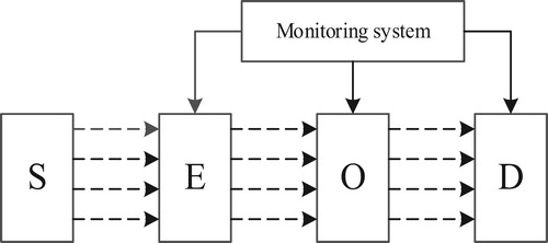
Figure 1. The processor structure of TOC. S: Surface light source, E: Encoder, O: Optical processor, D: Decoder.

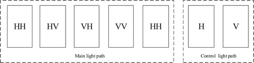
When applying the Decrease-Radix Design theory to TOC, there are 3⁹= 19,683 ternary logic operators and 18 basic operation units. And any ternary logic operation unit can be made of no more than 6 basic operation units. After deep research we found there is a uniform structure for the 18 basic operation units of the TOC as display in Figure 2. We can see in Figure 2, there are two optical paths: one is the main light path and the other is control light path. These two optical paths are composed of liquid crystal array, and they have different polarizers. The liquid crystal of the main light path is divided into four parts (HH, HV, VH, VV), and the liquid crystal of the control light path is divided into two parts (H, V), as shown in Figure 3 [22]. The input signal “a” enters the main optical path which involves two polarizers (P1 and P2) holding a liquid crystal (LC) to form a sandwich-like structure. Other input signal “b” enters the control optical path. The differences between basic operation units are that there are two opposite cases for the optical rotation of LC in static state, four combinations of P1’s and P2’s polarization directions, and three kinds of control optical paths. The three control optical paths are produced via dividing the input signal “b” into three sub-beams by two half-reflecting mirror f1, f2 and a mirror F. Because there is a vertical polarizer V in the top branch of the control optical path, the phototube g1 outputs high voltage only when the “b” is vertical polarized light. Similarly, for a horizontal polarizer H in middle branch, the g2 outputs high voltage only when the “b” is horizontal polarized light. And for no polarizer in the bottom branch, the g3 outputs high voltage when the “b” is bright whether vertical or horizontal polarized light. The device S (three choose one multiplexer) selects right one from the outputs of g1, g2 or g3 according to the reconfigure directive bits k2 and k3 and sends the right signal to XOR gate Y. The Y will negate the output signal of S when the reconfigure directive bit k1 is 1, and no negate when k1 is 0. The output signal of Y controls the optical rotation of the LC in main optical path [27]. So the output signal “c” is produced from the main optical path under the sway of the control optical path. The main optical path is split into four kinds in accordance with the combinations of P1’s and P2’s polarization directions. When P1 is vertical polarizer and P2 is horizontal polarizer the main optical path is called as VH; P1 is horizontal polarizer and P2 is vertical polarizer as HV. By that analogy, P1 and P2 are vertical polarizers as VV, and P1 and P2 are horizontal polarizers as HH.

Figure 2. Uniform structures of TOC’s basic operation units.

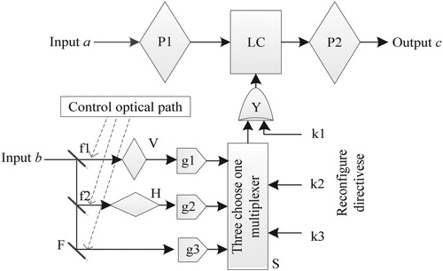
Figure 3. Optical processor light path division.

2.3.2. MSD adder

According to the Decrease-Radix Design principle disclosed in 2008 [17], any area of the data bits of the ternary optical processor can be reconstructed as a ternary (including binary) logic calculator at any time. However, the number of data bits cannot tolerate the delay of the carry process in the travelling wave adder, and it is difficult for the optical component to implement the carry tree structure in the carry lookahead of adder. Therefore, a numerical calculation system for the MSD counting system of TOC is established, which includes an MSD adder, a multiplication routine, a division routine and a matrix multiplication routine, in which MSD adder is the basis.

In 1961, Avizienis proposed an additive technique that can eliminate the carry delay—MSD (Modified Signed Digit) digital representation [32]. The MSD expression of A is (4) $A=\sum _i{k}_i{2}^i$(4) Among them, the domain of k_i∈{u, 0, 1}, u means −1; 2ⁱ indicates that MSD is also a binary counting method. Since k_i has three optional values, a decimal number can have multiple MSD representations. For convenience of description, the decimal number in this paper is labelled with subscript D, the MSD number is labelled with subscript M and the binary number is labelled with subscript B. The MSD addition includes T, W, T’, W’, T₂ (equivalent to T) five ternary logical transforms, as shown in Table 2. The operation process can be divided into three steps:

• Step 1: Apply operation T and W to the operands a and b bit by bit and append one 0 to the tail of the result of T.

• Step 2: Apply operation T’ and W’ separately to the result of T and result of W bit by bit. And append one 0 to the tail of the result of T’.

• Step 3: Apply operation T₂ which is the same to operation T to the results of T’ and result of W’ bit by bit. The result is the sum of the two.

Table 2. Truth table for T, W, T’, W’ and M transformations.

a	b	T	W	T’	W’	M
−1	−1	−1	0	−1	0	1
−1	0	−1	1	0	−1	0
−1	1	0	0	0	0	−1
0	−1	−1	1	0	−1	0
0	0	0	0	0	0	0
0	1	1	−1	0	1	0
1	−1	0	0	0	0	−1
1	0	1	−1	0	1	0
1	1	1	0	1	0	1

2.3.3. MSD multiplier

The logical operation corresponding to the multiplication of two MSD numbers is called M, and the truth table is shown in Table 2. When the n-digit data A = a_n-1 … a₁a₀ and B = b_n-1 … b₁b₀ are multiplied. Apply operation M to the ith digit data in the multiplier B and each digit data in the multiplicand A. The result is shifted to the left by i bits, and the result of the shift is called the partial product of the multiplication operation. The result of the accumulation of n partial products is the final result of the multiplication operation.

The accumulation process of n partial products is completed using a binary iteration method, and the operation steps are as follows:

1. The two adjacent partial products are input to an MSD adder to complete the operation. When n is an even number, the operation requires n/2 adders, and when n is an odd number, the operation requires n/2−1 adders. The result of the adder output is called partial sum.

2. Input the adjacent two partial sums into one MSD adder, and output the result as partial sum of the next operation.

3. Repeat the second step until there is only one partial sum, which is the MSD multiplication result.

3. Design of parallel ABC algorithm based on TOC

3.1. Design of parallel ABC algorithm

In the ABC algorithm, the employed bees and the onlooker bees need to search the neighbourhood of the food source and need to calculate a large number of fitness values. As the function dimension increases, it takes longer to calculate and search for fitness values. Through the performance test of the serial algorithm in 50 dimensions, the running time of the main function of the ABC algorithm is shown in Table 3.

Table 3. Performance analysis of serial ABC algorithm.

Function	CPU time (s)
SendOnlookerBees()	8.280
SendEmployedBees()	5.429
CalculateFitness()	0.132
main()	0.181
CalculateProbabilities()	0.179
MemorizeBestSource()	0.088
SendScoutBees()	0.032
init()	0.021

Table 4. Comparison of optimization results of test functions (D = 50).

Function	Algorithm	Variance	Maximum value	Minimum value
Sphere	ABC	1.24973E-13	4.21825E-13	2.6308E-15
	PABC	2.83156E-16	2.09483E-15	1.0321E-15
	TOC-PABC	4.24732E-17	2.37654E-15	3.01425E-16
Griewank	ABC	1.73325E-02	9.26400E-2	6.2477E-15
	PABC	2.14697E-09	9.34008E-06	0.0073E-16
	TOC-PABC	3.45854E-10	5.48962E-06	0.0051E-16
Rastrigin	ABC	0.46074	1.76652	4.7125E-12
	PABC	8.74712E-10	4.09921E-09	6.1497E-14
	TOC-PABC	6.37524E-12	2.34528E-09	4.2548E-11

Through the results of Table 3 and the study of the ABC algorithm, the most time-consuming part is: SendOnlookerBees function and SendEmployedBees function. Parallel design of ABC algorithm from the following sections:

1. Before the iterative loop of ABC, the entire population is initialized and then the fitness of these solutions is evaluated. The process of evaluating the fitness of all solutions is a cyclical calculation process. Each cycle is independent of each other, which satisfies the basic requirements of parallelism, so this phase can be processed in parallel.

2. In the process of finding the honey source by employed bees, each employed bee searches in its own area and its neighbours. The degree of dependence between employed bees is low, so there is natural parallelism. Initially, each honey source corresponds to an employed bee, and employed bee randomly searches for the vicinity of the honey source through Equation (2). Therefore, the search of employed bee can be performed on the TOC, and the main steps are as follows:

   • Step 1: Organize the position information and fitness value of the honey source into SZG file [11] and send the SZG file to the ternary optical processor (TOP).

   • Step 2: The TOP reconstructs n (depends on the size of the population) composite operators according to Equation (2), and employed bees searches the position information of the honey source in parallel randomly and calculates a new fitness value.

   • Step 3: Wait until the end of the search, greedy selection for the fitness value of each honey source, and compare the new fitness value with the old one, retain the honey source information with higher fitness value, and update the position information fitness value of the honey source in the global memory.

3. In the process of finding the honey source by onlooker bees, the selection process is a global probability selection, which is a global roulette selection method. According to the probability equation (3), a honey source is selected. And the onlooker bee is converted into an employed bee for neighbourhood search. This stage is completed on the TOC. Each bee completed the neighbourhood search and the new honey source fitness evaluation independently, so the onlooker bees’ stage also has parallelism. The specific steps are as follows:

   • Step 1: The TOP reconstructs n (depends on the size of the population) composite operators according to Equation (3), including the adder and the divider, and the onlooker bees selects a honey source by probability.

   • Step 2: The onlooker bees searches the position information of the honey source in parallel randomly and calculates a new fitness value.

   • Step 3: Wait until the end of the search, greedy selection for the fitness value of each honey source, and compare the new fitness value with the old one, retain the honey source information with higher fitness value, and update the position information fitness value of the honey source in the global memory.

4. At the end of the stage of the employed bees and the onlooker bees, detect all solutions that have not been updated. If the number of times a solution has not been updated exceeds the set threshold, the solution is discarded, and the scout bees will again find a new solution to replace the abandoned solution. This loop process is also independent of each other, so it can be processed in parallel.

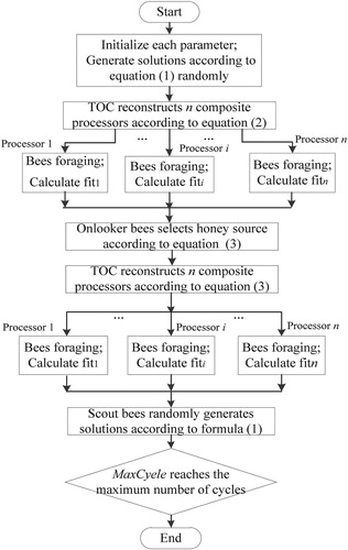
We maintain a master–slave parallel model with only one population without changing the basic structure of the ABC algorithm. The framework of the parallel ABC algorithm based on TOC is given, as shown in Figure 4.

Figure 4. Framework of the parallel ABC algorithm based on TOC.

3.2. Implementation of parallel ABC algorithm based on TOC

Combined with the above analysis, the specific implementation steps of the algorithm are as follows:

• Step 1: Initialize the parameters and evaluate the fitness value of the initial food source.

• Step 2: Using the Mason rotation algorithm to generate a 1024 × 1024 random number array on an electronic computer at one time and store it in the TOP.

• Step 3: Parallel method of searching for food sources by employed bees according to section (2) of 3.1. Each employed bee searches in the vicinity of the corresponding honey source and calculates the fitness value, and chooses the greedy value according to the fitness value. Update the location information and fitness value for the honey source that meets the conditions.

• Step 4: Parallel method of searching for food sources by onlooker bees according to section (3) of 3.1, onlooker bees select the food source to follow. Then the food source update process is completed on the TOC. Each onlooker bee searches in the vicinity of the corresponding honey source and calculates the fitness value, and chooses the greedy value according to the fitness value. Update the location information and fitness value for the honey source that meets the conditions.

• Step 5: If the food source is searched for more than a certain limit, and still has no honey source with higher fitness value, give up the honey source and generate a new honey source randomly.

• Step 6: Record the current global optimal solution and jump to step 2 until the maximum number of cycles maxCycle is reached. And send the final global optimal solution from the TOC to the CPU, output the final result.

3.3. Analysis of the clock cycle of algorithm

In the search phase of the employed bees, each employed bee finds a new honey source by Equation (2) v_ij= x_ij+ Ø_ij(x_ij – x_kj). By splitting Equation (2), it includes an addition, a subtraction and a multiplication. Addition uses a three-step adder, which requires three clock cycles to complete an addition. Since there is no sign bit in the MSD number, the subtraction is also implemented by the adder. It takes three clock cycles to complete one subtraction. One multiplication requires an M transform, which is one clock cycle, and requires ${\log }_2^{SN}$ layers of addition, that is 3log₂^SN clock cycles. Therefore, for a single calculation, a total of T = 7 + 3log₂^SN clock cycles are required.

In the search phase of the onlooker bees, the onlooker bees calculate the probability value of the food source selected by Equation (3). By analysing Equation (3), it contains SN consecutive additions and a division. On an electronic computer, SN consecutive additions require SN-1 calculations. However, on the TOC, when the processor bits are large enough, we can reconstruct ⌊SN/2⌋ adders. Partial sums are calculated by the binary iteration method, which requires [log₂^SN] calculations, which has great advantages in computing time compared to electronic computers.

4. Experiment and analysis

4.1. Experiment environment

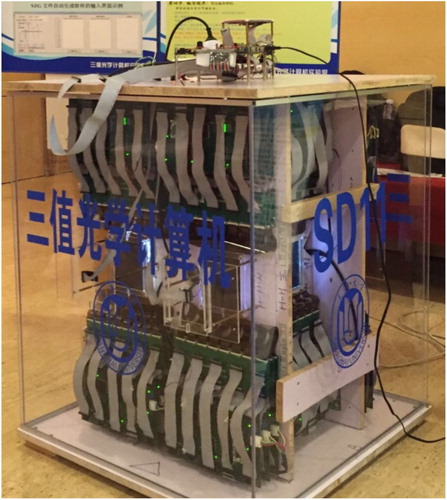
TOC environment configuration: This experiment uses the TOC prototype system – SD11 (for short SD11, means: Shanghai University 2011), the shape is shown in Figure 5. Among them, the liquid crystal (LC) array of the TOP (black area with bright spots in the middle) has 576 pixels arranged in a 24 × 24 array. The three adjacent pixels in each line form one bit of the optical processor, so the experimental device has a total of 192 processor bits, meaning that 192 bits of data can be processed in parallel. For more details about TOC, we recommend the interested readers to the literature [24].

Figure 5. SD11 experimental system.

Computer environment configuration: The hardware environment is AMD Athlon (tm) 64-bit Core Duo PC, memory 4G; the software environment is Microsoft Windows 7; the compilation environment is Visual Studio 2013, and the performance testing tool is Intel Parallel Studio.

4.2. Test benchmark functions and parameter setting

In the simulation experiment, the population size SN = 20, BN = SN/2, take D = 50 dimension and D = 100 dimension, maxCycle = 1000, limit = 100, and perform 30 times to find the average value independently. The experiment selects three classic Benchmark functions in the literature [33] for testing.

1. Sphere function: $f(x)\text{ }=\sum _{i=1}^n{x}_i^2,-100\le x_i\le 100$.

The Sphere function is a continuous unimodal function, which can well test the optimization accuracy of the algorithm [34]. The Sphere function reaches the minimum value of 0 when x_i= 0 (i = 1, 2, … , n).

1. Griewank function: $f(x)\text{ }=\frac{1}{\text{4000}}\sum _{i=1}^n{x}_i^2-{\prod }_{i=1}^n\cos (\frac{x_i}{\sqrt{i}})+1,\text{ }-600\le x_i\le 600$.

The Griewank function is a typical nonlinear multimodal function with a large number of local extremum points. With the function dimension increases, the number of local extremum points increases exponentially. The function has a wide search space, so it is usually considered to be a complex multimodal optimization problem that is difficult to handle by general optimization algorithms [34]. The function can well test the global search ability of the algorithm. The Griewank function reaches the minimum value of 0 when x_i= 0 (i = 1, 2, … , n).

1. Rastrigin function: $f(x)=\sum _{i=1}^n(x_i^2-10\cos (2\pi x_i)+10),\text{ }-5.12\le xi\le 5.12$.

The Rastrigin function is a multimodal function. There are approximately 10n (n is the dimension of the problem) local minimum point in the domain of the definition. It is a typical nonlinear multimodal function. The peak shape of the function is high and low fluctuations, so the general optimization algorithm is difficult to search for the global optimal value [34]. We use this function to detect the global optimization ability of the algorithm. The Rastrigin function reaches the minimum value of 0 when x_i= 0 (i = 1, 2, … , n).

4.3. Experimental results and analysis

Analysis 1: Tables 4 and Table 5 are the comparison results of the variance, the maximum value and the minimum value of the function in the case of D = 50 dimensions and D = 100 dimensions. The comparative algorithms are a serial ABC algorithm and a PABC algorithm implemented by an electronic computer, and a TOC-PABC algorithm implemented by TOC. It can be seen that the TOC-PABC algorithm is better than the ABC algorithm and the PABC algorithm, which fully demonstrates that the TOC-PABC algorithm has good global search performance.

Table 5. Comparison of optimization results of test functions (D = 100).

Function	Algorithm	Variance	Maximum value	Minimum value
Sphere	ABC	6.09423E-05	1.73493E-04	2.4776E-09
	PABC	2.49364E-15	0.04632E-12	4.0781E-13
	TOC-PABC	2.501275E-15	0.09564E-13	4.65872E-15
Griewank	ABC	4.68713	27.06907	8.64776
	PABC	0.79112E-08	2.98234E-05	0.7422E-15
	TOC-PABC	0.54821E-11	4.24598E-08	0.5412E-17
Rastrigin	ABC	0.00772	0.02930	6.4765E-07
	PABC	7.01312E-11	0.00973E-10	0.0004E-15
	TOC-PABC	6.54897E-16	0.00034E-10	0.0001E-20

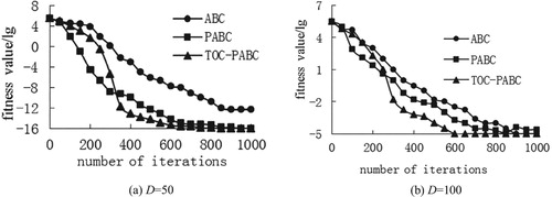
Analysis 2: It can be seen from Figure 6 that for the unimodal function Sphere, the PABC algorithm is slightly better than the ABC algorithm. When D = 50, the convergence speed of PABC and TOC-PABC algorithm is close, which does not reflect the efficiency of TOC-PABC algorithm, but the advantage of TOC-PABC algorithm appears in high-dimensional complex space.

Figure 6. Comparison of sphere functions in different dimensions.

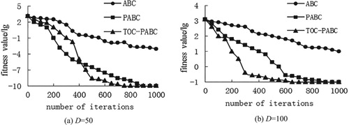
Analysis 3: From Figure 7(a) and Figure 8(a), the convergence speed and accuracy of the PABC algorithm are significantly higher than the ABC algorithm, and tend to be stable in the later stage. The TOC-PABC algorithm converges slightly slower in the early stage of evolution, but the convergence speed is significantly better than the first two algorithms in the later stage. It is concluded from Figure 7(b) and Figure 8(b) that the ABC algorithm converges very slowly in high-dimensional complex space, and there are almost no changes. However, the PABC algorithm and the TOC-PABC algorithm can quickly search for the optimal value. The optimization speed and stability of the TOC-PABC algorithm in the late evolution are obviously improved, and the Rastrigin function is particularly obvious.

Figure 7. Comparison of Griewank functions in different dimensions.

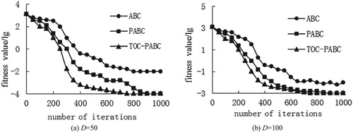
Figure 8. Comparison of Rastrigin functions in different dimensions.

Analysis 4: If the average running time of the ABC algorithm is Ts and the average running time of the TOC-PABC algorithm is Tp, the speedup Sp is: Sp = Ts/Tp. Table 6 shows the speedup of the two algorithms in 100 dimensions. It can be concluded that the parallel algorithm using TOC effectively improves the calculation performance and the speedup performance. Among them, the Griewank function has increased by more than 80%, and the other two algorithms have increased by nearly 70%, which is sufficient to illustrate the superiority of TOC in solving high-dimensional global problems with large search space.

Table 6. Speedup.

	Time (D = 100)
Function	ABC	TOC-PABC	Speedup
Sphere	0.00355	0.0013	1.677
Griewank	0.00643	0.00348	1.857
Rastrigin	0.00721	0.00425	1.683

Analysis 5: The TOC-PABC algorithm given in this paper is based on the TOC platform, which has many data bits and great potential for parallel computing. The TOC-PABC algorithm is improved by taking advantage of the highly parallel of TOC. On this basis, the differences between TOC-PABC and the traditional ABC algorithm are as follows:

1. In order to make full use of the parallel computing potential of TOC, through the parallel analysis of the various stages of the ABC algorithm, the TOC-PABC algorithm proposed in this paper adopts hardware parallel mode, which is supported by many data bits of TOC. For example, in the process of finding the honey source by onlooker bees, by decomposing the food source probability calculation formula and reconstructing the corresponding operator on the TOP, the onlooker bees can shorten the food source selection time to [log₂^SN]  clock cycles, while on the computer, it requires SN–1 consecutive calculations.

2. It is undeniable that the TOC-PABC algorithm increases the amount of calculation while reducing the clock cycle. However, the TOC-PABC algorithm keeps the required hardware resources within the acceptable range of the TOC while shortening the clock cycle. At present, this parallel scheme is difficult to implement for the ABC algorithm based on electronic computer.

3. Differences in the underlying platform lead to differences in algorithm performance. In the parallel TOC-PABC algorithm of this paper, the partial product of MSD multiplication is generated by the M operation in the ternary logic operation, and the partial product addition is realized by the MSD addition without carry. In the conventional method, the multiplication method uses bit and logic circuits or Booth coding circuits to generate partial products, and binary addition is used to realize partial product addition, which is a carry delay problem inevitably. This difference makes the time advantage of this paper more obvious when dealing with large quantities of data operations.

5. Conclusion

In this paper, the parallel ABC algorithm based on TOC is designed, and the implementation steps of the method are given. The correctness is proved by experiments. The effectiveness of the parallel strategy proposed in this paper is illustrated by comparing the algorithm clock cycle and comparing with the algorithm based on electronic computer. The realization method of improving the convergence time and search precision of ABC algorithm is analysed from a new perspective. It provides an effective means for the optimization problem of high-dimensional complex functions and also provides a new idea for parallel computing of other bionic algorithms.

Acknowledgement

Thanks to Prof. Jin Yi and all members from TOC research group for their suggestions and comments.

Disclosure statement

No potential conflict of interest was reported by the authors.

ORCID

Wenjing Li http://orcid.org/0000-0002-7230-3604

Additional information

Funding

This work is under the support of the National Natural Science Foundation of China [grant numbers 61866006, 61741203], Innovation Foundation of the Second Institute of China Aerospace Science and Technology Corporation, Natural Science Foundation of Shanghai [grant number15ZR1415400] and Special Research Program of Shanghai [grant number15700500400], Natural Science Foundation of Guangxi Province [grant number 2016GXNSFAA380243].

References

- Karaboga D. An idea based on bee swarm for numerical optimization, TR06. [S. l.]: Erciyes Univ. Engineering Faculty, Computer Engineering Department; 2005.
- Karaboga D, Akay B. A survey: algorithms simulating bee swarm intelligence. Artif Intell Rev. 2009;31(1-4):61–85. doi: 10.1007/s10462-009-9127-4
- Karaboga D, Akay B. A comparative study of artificial bee colony algorithm. Appl Math Comput. 2009;214(1):108–132.
- Karaboga D, Basturk B. A powerful and efficient algorithm for numerical function optimization: artificial bee colony (ABC) algorithm. J Global Optim. 2007;39(3):459–471. doi: 10.1007/s10898-007-9149-x
- Hu K, Li XB, Wang ZL. Performance of an improved artificial bee colony algorithm. J Comput App. 2011;31(4):1107–1110.
- Sun XY, Lin Y. Improved artificial bee colony algorithm for assignment problem. Microelectron Comp. 2012;29(1):23–26.
- Dong WY, Dong XS, Wang YF. Improved artificial bee colony algorithm for large scale colored bottleneck traveling salesman problem. J Commun. 2018;39(12):18–29.
- Liu XF, Liu PZ, Luo YM, et al. Improved artificial bee colony algorithm based on balanced search. J Huaqiao Univ Natural Sci. 2019;40(1):128–132.
- Jin Y, Ouyang S, Song K, et al. Management of many data bits in ternary optical computers. Sci China Sin Inf Sci. 2013;43(3):361–373.
- Ouyang S, Peng JJ, Jin Y, et al. Structure and theory of dual-space storage for ternary optical computer. Sci Sinica Inf Sci. 2016;46(6):743–762.
- Li S, Jin Y, Liu Y, et al. Initial SZG file generation software of the ternary optical computer. J Shanghai Univ Nat Sci. 2018;24(2):181–191.
- Li S, Jiang JB, Wang ZH, et al. Basic theory and key technology of programming platform of optical computer. Optik (Stuttg). 2019;178:327–336. doi: 10.1016/j.ijleo.2018.09.179
- Xu Q, Jin Y, Sheng YF, et al. MSD division algorithm and implementation technique for ternary optical computer. Sci China Ser F-Inf Sci. 2016;46(4):539–550.
- Li S, Jin Y. Simple structured data initial SZG files generation software design and implementation. Int Conf Wireless Commun Sens Netw. 2016;44:383–388.
- Gao H, Jin Y, Song K. Extension of C language in ternary optical computer. J Shanghai Univ Nat Sci. 2013;19(3):280–285.
- Zhang Q, Jin Y, Song K, et al. MPI programming based on ternary optical in supercomputer. J Shanghai Univ Nat Sci. 2014;20(2):180–189.
- Yan JY, Jin Y, Zuo KZ. Decrease-radix design principle for carrying/borrowing free multi-valued and application in ternary optical computer. Sci China Ser F. 2008;51(10):1415–1426.
- Jin Y, Gu YY, Zuo KZ. Theory, technology and progress of a ternary optical computer’s decoder. Sci China Ser F Inf Sci. 2013;43(2):275–286.
- Peng J, Wei X, Zhang X, et al. Implementation of parallel fft algorithm on ternary optical computer. Sci China Inf Sci. 2017;47(7):846–862.
- Peng J, Fu Y, Zhang X, et al. Implementation of dft application on ternary optical computer. Opt Commun. 2018;410:424–430. doi: 10.1016/j.optcom.2017.10.033
- Wang X, Zhang S, Zhang M, et al. Performance analysis of a ternary optical computer based on m/m/1 queuing system, in: 17th International Conference on Algorithms and Architectures for Parallel Processing, ICA3PP 2017 10393 LNCS 2017 pp. 331–344.
- Peng JJ, Shen R, Jin Y, et al. Design and implementation of modified signed-digit adder. IEEE Trans Comput. 2014;5(63):1134–1143. doi: 10.1109/TC.2012.285
- Peng JJ, Shen R, Ping XS. Design of a high-efficient MSD adder. J Supercomput. 2016;72(5):1770–1784. doi: 10.1007/s11227-015-1484-y
- Jin Y, Shen YF, Peng JJ, et al. Principles and construction of MSD adder in ternary optical computer. Sci China Inf Sci. 2010;53(11):2159–2168. doi: 10.1007/s11432-010-4091-9
- Shen YF, Pan L, Jin Y, et al. One-step binary MSD adder for ternary optical computer. Sci China Sin Inf Sci. 2012;42(7):869–881.
- Shen YF, Jiang B, Jin Y, et al. Principle and design of ternary optical accumulator implementing M-k-B addition. Opt Eng. 2014;53(9):1–8. doi: 10.1117/1.OE.53.9.095108
- Jin Y, Wang HJ, Ouyang S, et al. Principles, structures and implementation of reconfigurable ternary optical processors. Sci China Inf Sci. 2011;54(11):2236–2246. doi: 10.1007/s11432-011-4446-x
- Wang HJ, Jin Y, Ouyang S. Design and implementation of 1-bit reconfigurable ternary optical processor. Chin J Comput. 2014;37(7):1500–1507.
- Jin Y, Wang XC, Peng JJ, et al. Vector matrix multiplication in ternary optical computer. Int J Numer Anal Model. 2012;9(2):401–409.
- Wang XC, Peng JJ, Li M, et al. Carry-free vector-matrix multiplication on a dynamically reconfigurable optical platform. Appl Opt. 2010;49(12):2352–2362. doi: 10.1364/AO.49.002352
- Peng JJ, Teng L, Jin Y. Realization of a tri-valued programmable cellular automata with ternary optical computer. Int J Numer Anal Model. 2012;9(2):304–311.
- Avizienis A. Signed digit number representation for fast parallel arithmetic. IRE Trans Electr Comp. 1961;10(3):389–400. doi: 10.1109/TEC.1961.5219227
- Karaboga D, Basturk B. On the performance of artificial bee colony (ABC) algorithm. Appl Soft Comput. 2008;8(1):687–697. doi: 10.1016/j.asoc.2007.05.007
- He P. Research on Artificial Bee Colony Algorithm, Dissertation for Ph.D. degree, East China University of Science and Technology, Shanghai, 2013.