A gradient-based iterative algorithm for solving coupled Lyapunov equations of continuous-time Markovian jump systems

ABSTRACT

In this paper, a new gradient-based iterative algorithm is proposed to solve the coupled Lyapunov matrix equations associated with continuous-time Markovian jump linear systems. A necessary and sufficient condition is established for the proposed gradient-based iterative algorithm to be convergent. In addition, the optimal value of the tunable parameter achieving the fastest convergence rate of the proposed algorithm is given explicitly. Finally, some numerical simulations are given to validate the obtained theoretical results.

KEYWORDS:

• Coupled Lyapunov matrix equations
• iterative algorithms
• continuous-time Markovian jump systems

1. Introduction

Continuous-time Markovian jump linear systems have been widely used to describe some practical plants. Stability is fundamental for the investigation of any control systems. For the stability analysis of the Markovian jump linear systems, the coupled Lyapunov matrix equation is an important tool. In the past decades, the coupled continuous Lyapunov matrix equations are broadly used in stability analysis for continuous-time Markovian jump linear systems. In [1], the existence of the unique positive definite solution of coupled Lyapunov matrix equations was used to check the moment stability of Markovian jump linear systems. In [2], the authors shown that the Markovian jump linear system is stochastically stable if and only if the associated coupled Lyapunov matrix equation has a unique positive definite solution. The solution of the coupled Lyapunov matrix equations was used in [3] to check the stochastic stability of the nonhomogeneous Markovian jump system. In [4], the coupled Lyapunov equations have been applied to the stabilization of stochastic linear systems.

According to the above descriptions, it is known that the coupled Lyapunov matrix equation has an importance role in the stability analysis of the Markovian jump linear system. Thus, finding solutions for this kind of matrix equations has attracted much attention over the past decade. The exact solution of coupled continuous Lyapunov matrix equations was obtained in [5] by using the Kronecker product and matrix inversion. However, the computational difficulties of the traditional compute method will arise because excessive computer memory is required for computation of high-dimensional matrices. Due to this, the iterative approaches are widely used to solve coupled matrix equations in recently years and some effective iterative algorithms have been developed. For example, some gradient-based iterative algorithms were presented in [6,7] to solve the general coupled matrix equations, including the continuous coupled Lyapunov matrix equations. The reduced-rank gradient-based algorithm was developed in [8] for solving coupled Sylvester matrix equations. By using the property of symmetric positive definite matrix, a gradient-based iterative algorithm was presented in [9] for a type of coupled matrix equations. As a matter of fact, the above-mentioned gradient-based algorithms in [8,9] can also be extended to solve the coupled Lyapunov matrix equations. In addition, some explicit iterative algorithms are proposed to solve the coupled Lyapunov matrix equation. In [10], the conjugate direction method was given for solving the coupled Lyapunov matrix equations. In [11], a classical Smith iterative algorithm was constructed by using the fixed point iterative approach. A simple iterative technique was introduced in [12] to solve the coupled Lyapunov matrix equation. Recently, some new gradient-based iterative algorithms were presented for solving some kinds of matrix equations [13,14]. These algorithms also can be extended to solve the coupled Lyapunov matrix equations.

Besides, an implicit iterative algorithm was firstly proposed in [15] by taking the special structure of the coupled continuous-time Lyapunov matrix equations into consideration. In this algorithm, some standard continuous Lyapunov matrix equations need to be solved at each iteration step. Based on the idea in [15], two modified implicit iterative algorithms were developed in [16,17] for solving coupled continuous Lyapunov matrix equations. Recently, a new implicit iterative algorithm was constructed in [18] for solving the coupled Lyapunov matrix equation by using successive over relaxation. More results for the solution of the matrix equations can be found in [19–22]. However, some standard continuous Lyapunov matrix equations need to be solved in the aforementioned implicit iterative algorithms. In addition, a main disadvantage of the exist gradient-based iterative algorithms is that the convergence rates of these algorithms are slow. Inspired by the above analysis, in this paper, we aim to develop a new gradient-based iterative algorithm, which does not need to solve the standard Lyapunov equation and has faster convergence rate than the existing iterative algorithms.

In this paper, the gradient-based iterative technique is investigated for solving the continuous coupled Lyapunov matrix equations. First, a novel and simple gradient-based iterative algorithm is constructed and analysed. It is proven that the proposed gradient-based iterative algorithm converges to the unique solution of the coupled Lyapunov matrix equations if and only if the tunable parameter satisfies a certain inequality. Moreover, an optimal tunable value that achieves the fastest convergence rate of the algorithm is obtained. Finally, the correctiveness of the convergence results are verified by some simulation results.

Notation: Throughout this paper, the notation ⊗ represents the Kronecker product of two matrices. I represents an identity matrix of appropriate dimensions. For a real matrix A, we use $A^{\mathrm{T}},\parallel A{\parallel }_2,\parallel A{\parallel }_{\mathrm{F}},\lambda \left(A\right),{\lambda }_{min}\left(A\right),{\lambda }_{max}\left(A\right),$ and $\rho \left(A\right)$ to denote the transpose, the 2-norm, the $\mathrm{F}$-norm, the eigenvalues, the maximal eigenvalue, the minimal eigenvalue and the spectral radius of matrix A, respectively. For two integers m and l with $m\le l,$ $\mathbb{I}[m,l]$ denotes the set $\{m,m+1,\dots ,l\}.$ For two square matrices E and A, let us define $\lambda (E,A)=\{s|det(sE-A)=0\}.$ For any matrix $X=[x_1$ $x_2\cdots x_n]\in {\mathbb{R}}^{m\times n},$ the stretching function is defined as $\mathrm{v}\mathrm{e}\mathrm{c}(\cdot )=[x_1^{\mathrm{T}}$$x_2^{\mathrm{T}}\cdots x_n^{\mathrm{T}}].$

2. Preliminaries

Consider the following continuous-time Markovian jump linear system (1) $\mathrm{d}x\left(t\right)=A_{r\left(t\right)}x\left(t\right)\mathrm{d}t,$(1) where $x\left(t\right)\in {\mathbb{R}}^n$ is the system state, and $r\left(t\right)$ is a continuous-time discrete-state Markovian process taking values in a finite set $S\in \mathbb{I}[1,N]$. For the Markovian jump linear system (1(1) $\mathrm{d}x\left(t\right)=A_{r\left(t\right)}x\left(t\right)\mathrm{d}t,$(1) ), the system matrices of N subsystems are $A_i\in {\mathbb{R}}^{n\times n},i\in \mathbb{I}[1,N]$. The stationary transition probabilities of the Markovian process $r\left(t\right)$ are given by (2) $\begin{array}{rl}& \mathrm{P}\mathrm{r}\mathrm{o}\mathrm{b}\left(r\left(t+h\right)=j|r\left(t\right)=i\right)\\ & =\left\{\begin{array}{l}{\pi }_{ij}h+o\left(h\right),i\ne j,\\ 1+{\pi }_{ii}h+o\left(h\right),i=j,\end{array}\right.\end{array}$(2) where $h>0,\underset{h\to 0}{lim}o\left(h\right)/h=0$ and ${\pi }_{ij}$ ($j\ne i$) is the transition rate from mode i at time t to mode j at time t+h. All the transition rates ${\pi }_{ij}$, $i,j\in \mathbb{I}[1,N],$ can be collected into a transition rate matrix $\begin{array}{r}\mathrm{\Pi }=\left[\begin{array}{cccc}{\pi }_{11}& {\pi }_{12}& \cdots & {\pi }_{1N}\\ {\pi }_{21}& {\pi }_{22}& \cdots & {\pi }_{2N}\\ \cdots & \cdots & \ddots & \cdots \\ {\pi }_{N1}& {\pi }_{N2}& \cdots & {\pi }_{NN}\end{array}\right],\end{array}$ which has the following property $\begin{array}{rl}& {\pi }_{ij}\ge 0,i\ne j,\\ & {\pi }_{ij}<0,i=j,\\ & \sum _{j=1}^N{\pi }_{ij}=0.\end{array}$ Let the initial condition for the system (1(1) $\mathrm{d}x\left(t\right)=A_{r\left(t\right)}x\left(t\right)\mathrm{d}t,$(1) )–(2(2) $\begin{array}{rl}& \mathrm{P}\mathrm{r}\mathrm{o}\mathrm{b}\left(r\left(t+h\right)=j|r\left(t\right)=i\right)\\ & =\left\{\begin{array}{l}{\pi }_{ij}h+o\left(h\right),i\ne j,\\ 1+{\pi }_{ii}h+o\left(h\right),i=j,\end{array}\right.\end{array}$(2) ) be $x\left(0\right)=x_0$ and $r\left(0\right)=r_0,$ the definition of asymptotically mean square stability for the system (1(1) $\mathrm{d}x\left(t\right)=A_{r\left(t\right)}x\left(t\right)\mathrm{d}t,$(1) )–(2(2) $\begin{array}{rl}& \mathrm{P}\mathrm{r}\mathrm{o}\mathrm{b}\left(r\left(t+h\right)=j|r\left(t\right)=i\right)\\ & =\left\{\begin{array}{l}{\pi }_{ij}h+o\left(h\right),i\ne j,\\ 1+{\pi }_{ii}h+o\left(h\right),i=j,\end{array}\right.\end{array}$(2) ) can be stated as follows:

Definition 2.1

[3]

The continuous-time Markovian jump linear system (1(1) $\mathrm{d}x\left(t\right)=A_{r\left(t\right)}x\left(t\right)\mathrm{d}t,$(1) )–(2(2) $\begin{array}{rl}& \mathrm{P}\mathrm{r}\mathrm{o}\mathrm{b}\left(r\left(t+h\right)=j|r\left(t\right)=i\right)\\ & =\left\{\begin{array}{l}{\pi }_{ij}h+o\left(h\right),i\ne j,\\ 1+{\pi }_{ii}h+o\left(h\right),i=j,\end{array}\right.\end{array}$(2) ) is asymptotically mean square stable if for any $x_0\in {\mathbb{R}}^n,$ there holds $\underset{t\to \mathrm{\infty }}{lim}\mathrm{E}\left\{{∥x\left(t\right)∥}^2\right\}=0,$ where $\mathrm{E}$ the denotes mathematical expectation.

It is well known that the preceding mean square stability of the continuous-time Markovian jump linear system (1(1) $\mathrm{d}x\left(t\right)=A_{r\left(t\right)}x\left(t\right)\mathrm{d}t,$(1) )–(2(2) $\begin{array}{rl}& \mathrm{P}\mathrm{r}\mathrm{o}\mathrm{b}\left(r\left(t+h\right)=j|r\left(t\right)=i\right)\\ & =\left\{\begin{array}{l}{\pi }_{ij}h+o\left(h\right),i\ne j,\\ 1+{\pi }_{ii}h+o\left(h\right),i=j,\end{array}\right.\end{array}$(2) ) is closely related to the following continuous coupled Lyapunov matrix equations (CLMEs) (3) $A_i^{\mathrm{T}}{X}_i+X_i{A}_i+\sum _{j=1}^N{\pi }_{ij}{X}_j+Q_i=0,i\in \mathbb{I}\mathbb{[}1,N\mathbb{]},$(3) where $Q_i\in {\mathbb{R}}^{n\times n},i\in \mathbb{I}\mathbb{[}1,N]$, are arbitrarily given positive definite matrices, and $X_i,i\in \mathbb{I}\mathbb{[}1,N]$, are the unknown matrices to be determined. Regarding the mean square stability of the system (1(1) $\mathrm{d}x\left(t\right)=A_{r\left(t\right)}x\left(t\right)\mathrm{d}t,$(1) )–(2(2) $\begin{array}{rl}& \mathrm{P}\mathrm{r}\mathrm{o}\mathrm{b}\left(r\left(t+h\right)=j|r\left(t\right)=i\right)\\ & =\left\{\begin{array}{l}{\pi }_{ij}h+o\left(h\right),i\ne j,\\ 1+{\pi }_{ii}h+o\left(h\right),i=j,\end{array}\right.\end{array}$(2) ), the following results are introduced.

Lemma 2.1

[3]

The continuous-time Markovian jump linear system (1(1) $\mathrm{d}x\left(t\right)=A_{r\left(t\right)}x\left(t\right)\mathrm{d}t,$(1) )–(2(2) $\begin{array}{rl}& \mathrm{P}\mathrm{r}\mathrm{o}\mathrm{b}\left(r\left(t+h\right)=j|r\left(t\right)=i\right)\\ & =\left\{\begin{array}{l}{\pi }_{ij}h+o\left(h\right),i\ne j,\\ 1+{\pi }_{ii}h+o\left(h\right),i=j,\end{array}\right.\end{array}$(2) ) is mean square stable if and only if the continuous CLMEs (3(3) $A_i^{\mathrm{T}}{X}_i+X_i{A}_i+\sum _{j=1}^N{\pi }_{ij}{X}_j+Q_i=0,i\in \mathbb{I}\mathbb{[}1,N\mathbb{]},$(3) ) have a unique solution $\mathcal{X}=(X_1,X_2,\dots ,X_N)$ with $X_i>0,i\in \mathbb{I}\mathbb{[}1,N]$, for any given $\mathcal{Q}=(Q_1,Q_2,\dots ,Q_N)$ with $Q_i>0,i\in \mathbb{I}\mathbb{[}1,N]$.

Due to the significance of the continuous CLMEs in the stability analysis of the Markovian jump linear system, many researchers pay attention to the solution of the continuous CLMEs (3(3) $A_i^{\mathrm{T}}{X}_i+X_i{A}_i+\sum _{j=1}^N{\pi }_{ij}{X}_j+Q_i=0,i\in \mathbb{I}\mathbb{[}1,N\mathbb{]},$(3) ). In next section, we will investigate the iterative technique for solving the continuous CLMEs (3(3) $A_i^{\mathrm{T}}{X}_i+X_i{A}_i+\sum _{j=1}^N{\pi }_{ij}{X}_j+Q_i=0,i\in \mathbb{I}\mathbb{[}1,N\mathbb{]},$(3) ). Before give the main results, we first present some classical iterative algorithms.

Algorithm 2.1

[16]

(4) $\begin{array}{rl}& {\left(A_i+\left({\pi }_{ii}/2\right)I\right)}^{\mathrm{T}}{X}_i\left(k+1\right)\\ & +X_i\left(k+1\right)\left(A_i+\left({\pi }_{ii}/2\right)I\right)\\ & =-\sum _{j=1}^{i-1}{\pi }_{ij}{X}_j\left(k+1\right)\\ & -\sum _{j=i+1}^N{\pi }_{ij}{X}_j\left(k\right)-Q_i,i\in \mathbb{I}\mathbb{[}1,N\mathbb{]}.\end{array}$(4)

Algorithm 2.2

[17]

(5) $\begin{array}{rl}& {\left[A_i+\left({\pi }_{ii}/2\right)I-\left({\omega }_i/2\right)I\right]}^{\mathrm{T}}{X}_i\left(k+1\right)\\ & +X_i\left(k+1\right)\left[A_i+\left({\pi }_{ii}/2\right)I-\left({\omega }_i/2\right)I\right]\\ & =-\sum _{j=1}^{i-1}{\pi }_{ij}\left(\sum _{t=0}^{s_{ij}}{\gamma }_{ijt}{X}_j\left(k+1-t\right)\right)\\ & -{\omega }_i\left(\sum _{t=0}^{s_{ij}}{\gamma }_{ijt}{X}_j\left(k-t\right)\right)\\ & -\sum _{j=i+1}^N{\pi }_{ij}\left(\sum _{t=0}^{s_{ij}}{\gamma }_{ijt}{X}_j\left(k-t\right)\right)-Q_i,i\in \mathbb{I}\mathbb{[}1,N\mathbb{]},\end{array}$(5) where ${\gamma }_{ijt},t\in \mathbb{I}\mathbb{[}0,s_{ij}]$, $i,j\in \mathbb{I}\mathbb{[}1,N]$, and ${\omega }_i,i\in \mathbb{I}\mathbb{[}1,N],$ are some tunable parameters, which satisfy some given conditions.

In this paper, k denotes the iterative step of the iterative algorithms.

Remark 2.1

For Algorithms 2.1 and 2.2, at each iteration step, one needs to solve N standard continuous Lyapunov matrix equations in the following form, $A^{\mathrm{T}}X+XA=-Q.$ Due to this, some additional operations are required when using Algorithms 2.1 and 2.2 for solving the continuous CLMEs (3(3) $A_i^{\mathrm{T}}{X}_i+X_i{A}_i+\sum _{j=1}^N{\pi }_{ij}{X}_j+Q_i=0,i\in \mathbb{I}\mathbb{[}1,N\mathbb{]},$(3) ). Thus, they are implicit iterative algorithms.

In addition, the gradient-based iterative algorithms proposed in [7,8] can also be used to solve the continuous CLMEs (3(3) $A_i^{\mathrm{T}}{X}_i+X_i{A}_i+\sum _{j=1}^N{\pi }_{ij}{X}_j+Q_i=0,i\in \mathbb{I}\mathbb{[}1,N\mathbb{]},$(3) ). These results are stated as follows:

Algorithm 2.3

[7]

(6) $\begin{array}{rl}& X_i\left(k+1\right)=X_i\left(k\right)\\ & -\mu \left(A_i^{\mathrm{T}}{T}_i\left(X\right)+T_i\left(X\right)A_i+\sum _{i=1}^N{\pi }_{ij}{T}_i\left(X\right)\right),\end{array}$(6) with (7) $\begin{array}{rl}{T}_i\left(X\right)& =A_i^{\mathrm{T}}{X}_i\left(k\right)+X_i\left(k\right)A_i\\ & +\sum _{j=1}^N{\pi }_{ij}{X}_j\left(k\right)+Q_i,i\in \mathbb{I}\mathbb{[}1,N\mathbb{]}.\end{array}$(7)

Algorithm 2.4

[8]

(8) $\begin{array}{rl}{Y}_i\left(k+1\right)& =Y_i\left(k\right)-\mu \left(\phantom{\sum _{j=1}^N{\pi }_{ij}{X}_j\left(Y\right(k\left)\right)+Q_i}{A}_i^{\mathrm{T}}{X}_i\left(Y\right(k\left)\right)+X_i\left(Y\right(k\left)\right)A_i\right.\\ & \left.+\sum _{j=1}^N{\pi }_{ij}{X}_j\left(Y\right(k\left)\right)+Q_i\right),i\in \mathbb{I}[1,N],\end{array}$(8) where $\begin{array}{rl}{X}_j\left(Y\right(k\left)\right)& =A_j^{\mathrm{T}}{Y}_j\left(k\right)+Y_j\left(k\right)A_j\\ & +\sum _{i=1}^N{\pi }_{ij}{Y}_i\left(k\right),j\in \mathbb{I}[1,N].\end{array}$

Remark 2.2

It is easily noted that the gradient-based iterative Algorithms 2.3 and 2.4 involve intermediate variables $T_i\left(k\right)$ and $Y_i\left(k\right)$ at each iterative step. Thus, the computational cost of these two gradient-based iterative algorithms are high.

In this section, two explicit iterative algorithms and two implicit iterative algorithms for solving the continuous CLMEs (3(3) $A_i^{\mathrm{T}}{X}_i+X_i{A}_i+\sum _{j=1}^N{\pi }_{ij}{X}_j+Q_i=0,i\in \mathbb{I}\mathbb{[}1,N\mathbb{]},$(3) ) have been reviewed. In order to improve the convergence rate, a new gradient-based iterative algorithm to solve the continuous CLMEs (3(3) $A_i^{\mathrm{T}}{X}_i+X_i{A}_i+\sum _{j=1}^N{\pi }_{ij}{X}_j+Q_i=0,i\in \mathbb{I}\mathbb{[}1,N\mathbb{]},$(3) ) will be proposed in the next section.

3. A new gradient-based iterative algorithm

The basic idea of the gradient-based iterative method is to search for an optimal matrix $\mathcal{X}=(X_1,X_2,\dots ,X_N)$ such that a given objective function is minimized. In this case, some simplified objective functions can be given as follows: (9) $\begin{array}{rl}{J}_i\left(X\right)& =\frac{1}{2}{∥A_i^{\mathrm{T}}{X}_i+X_i{A}_i+\sum _{j=1}^N{\pi }_{ij}{X}_j+Q_i∥}_{\mathrm{F}}^2,\\ & i\in \mathbb{I}\mathbb{[}1,N\mathbb{]}.\end{array}$(9) To construct the gradient-based iterative algorithm, we should first calculate the gradient of $J_i\left(X\right),i\in \mathbb{I}\mathbb{[}1,N\mathbb{]}$, with respect to $X_i,i\in \mathbb{I}\mathbb{[}1,N]$. In fact, the gradient of $J_i\left(X\right),i\in \mathbb{I}\mathbb{[}1,N]$, with respect to $X_i,i\in \mathbb{I}\mathbb{[}1,N]$, can be derived easily as below: (10) $\frac{\mathrm{\partial }{J}_i\left(X\right)}{\mathrm{\partial }{X}_i}=A_i^{\mathrm{T}}{T}_i+T_i{A}_i+{\pi }_{ii}{T}_i,$(10) where $T_i,i\in \mathbb{I}\mathbb{[}1,N]$, are given by (11) $T_i=A_i^{\mathrm{T}}{X}_i+X_i{A}_i+\sum _{j=1}^N{\pi }_{ij}{X}_j+Q_i.$(11) Now, based on (10(10) $\frac{\mathrm{\partial }{J}_i\left(X\right)}{\mathrm{\partial }{X}_i}=A_i^{\mathrm{T}}{T}_i+T_i{A}_i+{\pi }_{ii}{T}_i,$(10) ) a new gradient-based iterative algorithm can be constructed to search the solution of the continuous CLMEs (3(3) $A_i^{\mathrm{T}}{X}_i+X_i{A}_i+\sum _{j=1}^N{\pi }_{ij}{X}_j+Q_i=0,i\in \mathbb{I}\mathbb{[}1,N\mathbb{]},$(3) ).

Algorithm 3.1

(12) $\begin{array}{rl}& X_i\left(k+1\right)\\ & =X_i\left(k\right)-\mu \left(A_i^{\mathrm{T}}{T}_i\left(X\right)+T_i\left(X\right)A_i+{\pi }_{ii}{T}_i\left(X\right)\right),\\ & i\in \mathbb{I}\mathbb{[}1,N\mathbb{]},\end{array}$(12) where $T_i\left(X\right),i\in \mathbb{I}\mathbb{[}1,N]$, are defined in (7(7) $\begin{array}{rl}{T}_i\left(X\right)& =A_i^{\mathrm{T}}{X}_i\left(k\right)+X_i\left(k\right)A_i\\ & +\sum _{j=1}^N{\pi }_{ij}{X}_j\left(k\right)+Q_i,i\in \mathbb{I}\mathbb{[}1,N\mathbb{]}.\end{array}$(7) ).

Remark 3.1

In comparison with the existing Algorithms 2.1 and 2.2, the proposed Algorithm 3.1 is explicit and it does not need to solve the standard Lyapunov matrix equations by applying the Matlab function 'lyap'. Thus, the computational cost of the Algorithm 3.1 should be less than the implicit iterative Algorithms 2.1 and 2.2.

Remark 3.2

In comparison with the existing Algorithms 2.3 and 2.4, it can be observed that the term ${\displaystyle \sum _{i=1,i\ne j}^N{\pi }_{ij}{T}_i\left(X\right)}$ is not included in the Algorithm 3.1 at each iterative step. In this case, the computational complexity of this gradient-based algorithm will be much lower than the existing iterative algorithms. Therefore, the proposed Algorithm 3.1 would have faster convergence rate than the Algorithms 2.3 and 2.4 as evidenced in the simulations.

In the following, we will give some convergence results of the Algorithm 3.1. To this end, we first introduce the following useful lemma, which has an important role in the derivation of the main results.

Lemma 3.1

[23]

If $A\in {\mathbb{R}}^{m\times n},B\in {\mathbb{R}}^{p\times q},$ and $X\in {\mathbb{R}}^{n\times p},$ then we have $\mathrm{v}\mathrm{e}\mathrm{c}\left(AXB\right)=\left(B^{\mathrm{T}}\otimes A\right)\mathrm{v}\mathrm{e}\mathrm{c}\left(X\right).$

In addition, it is denoted that (13) $\begin{array}{rl}\mathrm{\Omega }& =\left[\begin{array}{ccc}{\mathrm{\Psi }}_1^2& {\pi }_{12}{\mathrm{\Psi }}_1& \cdots \\ {\pi }_{21}{\mathrm{\Psi }}_2& {\mathrm{\Psi }}_2^2& {\pi }_{23}{\mathrm{\Psi }}_2\\ \cdots & \cdots & \ddots \\ {\pi }_{N-1,1}{\mathrm{\Psi }}_{N-1}& \cdots & \cdots \\ {\pi }_{N1}{\mathrm{\Psi }}_N& \cdots & \cdots \end{array}\right.,\\ & \left.\begin{array}{cc}\cdots & {\pi }_{1N}{\mathrm{\Psi }}_1\\ \cdots & {\pi }_{2N}{\mathrm{\Psi }}_2\\ \cdots & \cdots \\ {\mathrm{\Psi }}_{N-1}^2& {\pi }_{N-1,N}{\mathrm{\Psi }}_{N-1}\\ {\pi }_{N,N-1}{\mathrm{\Psi }}_N& {\mathrm{\Psi }}_N^2\end{array}\right],\end{array}$(13) where (14) $\begin{array}{rl}{\mathrm{\Psi }}_i& =I\otimes {\left(A_i+\left({\pi }_{ii}/2\right)I\right)}^{\mathrm{T}}\\ & +{\left(A_i+\left({\pi }_{ii}/2\right)I\right)}^{\mathrm{T}}\otimes I,i\in \mathbb{I}\mathbb{[}1,N\mathbb{]},\end{array}$(14) and let (15) $\lambda \left(\mathrm{\Omega }\right)=\left\{c_1+d_1\mathrm{i},c_2+d_2\mathrm{i},\dots ,c_{n^{2}N}+d_{n^{2}N}\mathrm{i}\right\},$(15) where $c_i,d_i\in \mathbb{R},i\in \mathbb{I}\mathbb{[}1,n^{2}N]$. On the basis of above notations (13(13) $\begin{array}{rl}\mathrm{\Omega }& =\left[\begin{array}{ccc}{\mathrm{\Psi }}_1^2& {\pi }_{12}{\mathrm{\Psi }}_1& \cdots \\ {\pi }_{21}{\mathrm{\Psi }}_2& {\mathrm{\Psi }}_2^2& {\pi }_{23}{\mathrm{\Psi }}_2\\ \cdots & \cdots & \ddots \\ {\pi }_{N-1,1}{\mathrm{\Psi }}_{N-1}& \cdots & \cdots \\ {\pi }_{N1}{\mathrm{\Psi }}_N& \cdots & \cdots \end{array}\right.,\\ & \left.\begin{array}{cc}\cdots & {\pi }_{1N}{\mathrm{\Psi }}_1\\ \cdots & {\pi }_{2N}{\mathrm{\Psi }}_2\\ \cdots & \cdots \\ {\mathrm{\Psi }}_{N-1}^2& {\pi }_{N-1,N}{\mathrm{\Psi }}_{N-1}\\ {\pi }_{N,N-1}{\mathrm{\Psi }}_N& {\mathrm{\Psi }}_N^2\end{array}\right],\end{array}$(13) ) and (15(15) $\lambda \left(\mathrm{\Omega }\right)=\left\{c_1+d_1\mathrm{i},c_2+d_2\mathrm{i},\dots ,c_{n^{2}N}+d_{n^{2}N}\mathrm{i}\right\},$(15) ), a necessary and sufficient condition for the convergence of the proposed Algorithm 3.1 can be given in the following theorem.

Theorem 3.1

Assume that the continuous CLMEs (3(3) $A_i^{\mathrm{T}}{X}_i+X_i{A}_i+\sum _{j=1}^N{\pi }_{ij}{X}_j+Q_i=0,i\in \mathbb{I}\mathbb{[}1,N\mathbb{]},$(3) ) has a unique solution $\mathcal{X}=(X_1,X_2,\dots ,X_N)$.

If (16) $c_i>0,\mathrm{\forall }i\in \mathbb{I}\mathbb{[}1,n^{2}N\mathbb{]},$(16) then, the sequence $\mathcal{X}\left(k\right)=\left(X_1\right(k),X_2(k),\dots ,X_N(k\left)\right)$ obtained by the Algorithm 3.1 with arbitrary initial condition converges to the unique solution of CLMEs (3(3) $A_i^{\mathrm{T}}{X}_i+X_i{A}_i+\sum _{j=1}^N{\pi }_{ij}{X}_j+Q_i=0,i\in \mathbb{I}\mathbb{[}1,N\mathbb{]},$(3) ) if and only if (17) $0<\mu <\frac{2c_i}{c_i^2+d_i^2},\mathrm{\forall }i\in \mathbb{I}\mathbb{[}1,n^{2}N\mathbb{]};$(17) If (18) $c_i<0,\mathrm{\forall }i\in \mathbb{I}\mathbb{[}1,n^{2}N\mathbb{]},$(18) then, the sequence $\mathcal{X}\left(k\right)=\left(X_1\right(k),X_2(k),\dots ,X_N(k\left)\right)$ obtained by the Algorithm 3.1 with arbitrary initial condition converges to the unique solution of CLMEs (3(3) $A_i^{\mathrm{T}}{X}_i+X_i{A}_i+\sum _{j=1}^N{\pi }_{ij}{X}_j+Q_i=0,i\in \mathbb{I}\mathbb{[}1,N\mathbb{]},$(3) ) if and only if (19) $\frac{2c_i}{c_i^2+d_i^2}<\mu <0,\mathrm{\forall }i\in \mathbb{I}\mathbb{[}1,n^{2}N\mathbb{]}.$(19) If neither the condition (16(16) $c_i>0,\mathrm{\forall }i\in \mathbb{I}\mathbb{[}1,n^{2}N\mathbb{]},$(16) ) nor the condition (18(18) $c_i<0,\mathrm{\forall }i\in \mathbb{I}\mathbb{[}1,n^{2}N\mathbb{]},$(18) ) is satisfied, then the Algorithm 3.1 is divergent.

Proof.

Define the iterative error matrix (20) ${\tilde{X}}_i\left(k\right)=X_i\left(k\right)-X_i,i\in \mathbb{I}\mathbb{[}1,N\mathbb{]}.$(20) Substituting (21) $Q_i=-A_i^{\mathrm{T}}{X}_i-X_i{A}_i-\sum _{j=1}^N{\pi }_{ij}{X}_j,i\in \mathbb{I}\mathbb{[}1,N\mathbb{]},$(21) into the Algorithm 3.1 and adding $-X_i,i\in \mathbb{I}\mathbb{[}1,N]$, on both sides of (12(12) $\begin{array}{rl}& X_i\left(k+1\right)\\ & =X_i\left(k\right)-\mu \left(A_i^{\mathrm{T}}{T}_i\left(X\right)+T_i\left(X\right)A_i+{\pi }_{ii}{T}_i\left(X\right)\right),\\ & i\in \mathbb{I}\mathbb{[}1,N\mathbb{]},\end{array}$(12) ), yields (22) $\begin{array}{rl}{\tilde{X}}_i\left(k+1\right)& ={\tilde{X}}_i\left(k\right)-\mu \left[{\left(A_i+\left({\pi }_{ii}/2\right)I\right)}^{\mathrm{T}}{T}_i\left(\tilde{X}\right)\right.\\ & \left.+T_i\left(\tilde{X}\right)\left(A_i+\left({\pi }_{ii}/2\right)I\right)\phantom{{\left(A_i+\left({\pi }_{ii}/2\right)I\right)}^{\mathrm{T}}{T}_i\left(\tilde{X}\right)}\right],i\in \mathbb{I}\mathbb{[}1,N\mathbb{]},\end{array}$(22) with $\begin{array}{rl}{T}_i\left(\tilde{X}\right)& ={\left(A_i+\left({\pi }_{ii}/2\right)I\right)}^{\mathrm{T}}{\tilde{X}}_i\left(k\right)\\ & +{\tilde{X}}_i\left(k\right)\left(A_i+\left({\pi }_{ii}/2\right)I\right)\\ & +\sum _{j=1,j\ne i}^N{\pi }_{ij}{\tilde{X}}_j\left(k\right),i\in \mathbb{I}\mathbb{[}1,N\mathbb{]},\end{array}$ where ${\tilde{X}}_i\left(k\right),i\in \mathbb{I}\mathbb{[}1,N]$, are defined in (20(20) ${\tilde{X}}_i\left(k\right)=X_i\left(k\right)-X_i,i\in \mathbb{I}\mathbb{[}1,N\mathbb{]}.$(20) ). Next, by performing vectorization operation and using Lemma 3.1, the obtained expressions (22(22) $\begin{array}{rl}{\tilde{X}}_i\left(k+1\right)& ={\tilde{X}}_i\left(k\right)-\mu \left[{\left(A_i+\left({\pi }_{ii}/2\right)I\right)}^{\mathrm{T}}{T}_i\left(\tilde{X}\right)\right.\\ & \left.+T_i\left(\tilde{X}\right)\left(A_i+\left({\pi }_{ii}/2\right)I\right)\phantom{{\left(A_i+\left({\pi }_{ii}/2\right)I\right)}^{\mathrm{T}}{T}_i\left(\tilde{X}\right)}\right],i\in \mathbb{I}\mathbb{[}1,N\mathbb{]},\end{array}$(22) ) can be equivalently written as $\begin{array}{rl}& \mathrm{v}\mathrm{e}\mathrm{c}\left({\tilde{X}}_i\left(k+1\right)\right)=\mathrm{v}\mathrm{e}\mathrm{c}\left({\tilde{X}}_i\left(k\right)\right)\\ & -\mu \left[(I\otimes {\left(A_i+\left({\pi }_{ii}/2\right)I\right)}^{\mathrm{T}})\mathrm{v}\mathrm{e}\mathrm{c}\left(T_i\right(\tilde{X}\left)\right)\right.\\ & \left.+({\left(A_i+\left({\pi }_{ii}/2\right)I\right)}^{\mathrm{T}}\otimes I)\mathrm{v}\mathrm{e}\mathrm{c}\left(T_i\right(\tilde{X}\left)\right)\right],\\ & i\in \mathbb{I}\mathbb{[}1,N\mathbb{]},\end{array}$ with $\begin{array}{rl}\mathrm{v}\mathrm{e}\mathrm{c}\left(T_i\right(\tilde{X}\left)\right)& =(I\otimes {\left(A_i+\left({\pi }_{ii}/2\right)I\right)}^{\mathrm{T}})\mathrm{v}\mathrm{e}\mathrm{c}\left({\tilde{X}}_i\left(k\right)\right)\\ & +({\left(A_i+\left({\pi }_{ii}/2\right)I\right)}^{\mathrm{T}}\otimes I)\mathrm{v}\mathrm{e}\mathrm{c}\left({\tilde{X}}_i\left(k\right)\right)\\ & +\sum _{j=1,j\ne i}^N{\pi }_{ij}\mathrm{v}\mathrm{e}\mathrm{c}\left({\tilde{X}}_j\left(k\right)\right),i\in \mathbb{I}\mathbb{[}1,N\mathbb{]},\end{array}$ Further, by using the notation (14(14) $\begin{array}{rl}{\mathrm{\Psi }}_i& =I\otimes {\left(A_i+\left({\pi }_{ii}/2\right)I\right)}^{\mathrm{T}}\\ & +{\left(A_i+\left({\pi }_{ii}/2\right)I\right)}^{\mathrm{T}}\otimes I,i\in \mathbb{I}\mathbb{[}1,N\mathbb{]},\end{array}$(14) ), it can be obtained from the above equations that $\begin{array}{rl}\mathrm{v}\mathrm{e}\mathrm{c}\left({\tilde{X}}_i\left(k+1\right)\right)& =\mathrm{v}\mathrm{e}\mathrm{c}\left({\tilde{X}}_i\left(k\right)\right)\\ & -\mu \left[{\mathrm{\Psi }}_i\mathrm{v}\mathrm{e}\mathrm{c}\left(T_i\right(\tilde{X}\left)\right)\right],i\in \mathbb{I}\mathbb{[}1,N\mathbb{]},\end{array}$ with $\begin{array}{rl}\mathrm{v}\mathrm{e}\mathrm{c}\left(T_i\right(\tilde{X}\left)\right)& ={\mathrm{\Psi }}_i\mathrm{v}\mathrm{e}\mathrm{c}\left({\tilde{X}}_i\left(k\right)\right)\\ & +\sum _{j=1,j\ne i}^N{\pi }_{ij}\mathrm{v}\mathrm{e}\mathrm{c}\left({\tilde{X}}_j\left(k\right)\right),i\in \mathbb{I}\mathbb{[}1,N\mathbb{]},\end{array}$ where ${\mathrm{\Psi }}_i,i\in \mathbb{I}\mathbb{[}1,N]$, are defined in (14(14) $\begin{array}{rl}{\mathrm{\Psi }}_i& =I\otimes {\left(A_i+\left({\pi }_{ii}/2\right)I\right)}^{\mathrm{T}}\\ & +{\left(A_i+\left({\pi }_{ii}/2\right)I\right)}^{\mathrm{T}}\otimes I,i\in \mathbb{I}\mathbb{[}1,N\mathbb{]},\end{array}$(14) ). From the above equations, one can obtain $\begin{array}{rl}\mathrm{v}\mathrm{e}\mathrm{c}\left({\tilde{X}}_i\left(k+1\right)\right)& =\mathrm{v}\mathrm{e}\mathrm{c}\left({\tilde{X}}_i\left(k\right)\right)-\mu \left[\phantom{{\mathrm{\Psi }}_i\sum _{j=1,j\ne i}^N{\pi }_{ij}\mathrm{v}\mathrm{e}\mathrm{c}\left({\tilde{X}}_j\left(k\right)\right)}{\mathrm{\Psi }}_i^2\mathrm{v}\mathrm{e}\mathrm{c}\left({\tilde{X}}_i\left(k\right)\right)\right.\\ & \left.+{\mathrm{\Psi }}_i\sum _{j=1,j\ne i}^N{\pi }_{ij}\mathrm{v}\mathrm{e}\mathrm{c}\left({\tilde{X}}_j\left(k\right)\right)\right].\end{array}$ Then, the above relations can be compactly written as (23) $\tilde{\eta }\left(k+1\right)=\left(I-\mu \mathrm{\Omega }\right)\tilde{\eta }\left(k\right),$(23) where Ω is defined in (13(13) $\begin{array}{rl}\mathrm{\Omega }& =\left[\begin{array}{ccc}{\mathrm{\Psi }}_1^2& {\pi }_{12}{\mathrm{\Psi }}_1& \cdots \\ {\pi }_{21}{\mathrm{\Psi }}_2& {\mathrm{\Psi }}_2^2& {\pi }_{23}{\mathrm{\Psi }}_2\\ \cdots & \cdots & \ddots \\ {\pi }_{N-1,1}{\mathrm{\Psi }}_{N-1}& \cdots & \cdots \\ {\pi }_{N1}{\mathrm{\Psi }}_N& \cdots & \cdots \end{array}\right.,\\ & \left.\begin{array}{cc}\cdots & {\pi }_{1N}{\mathrm{\Psi }}_1\\ \cdots & {\pi }_{2N}{\mathrm{\Psi }}_2\\ \cdots & \cdots \\ {\mathrm{\Psi }}_{N-1}^2& {\pi }_{N-1,N}{\mathrm{\Psi }}_{N-1}\\ {\pi }_{N,N-1}{\mathrm{\Psi }}_N& {\mathrm{\Psi }}_N^2\end{array}\right],\end{array}$(13) ) and (24) $\begin{array}{rl}\tilde{\eta }\left(k\right)& =\left[{\left[\mathrm{v}\mathrm{e}\mathrm{c}\left({\tilde{X}}_1\left(k\right)\right)\right]}^{\mathrm{T}}{\left[\mathrm{v}\mathrm{e}\mathrm{c}\left({\tilde{X}}_2\left(k\right)\right)\right]}^{\mathrm{T}}\cdots \right.\\ & {\left.{\left[\mathrm{v}\mathrm{e}\mathrm{c}\left({\tilde{X}}_N\left(k\right)\right)\right]}^{\mathrm{T}}\right]}^{\mathrm{T}}.\end{array}$(24) This relation implies that $\underset{k\to \mathrm{\infty }}{lim}{\tilde{X}}_i\left(k\right)=0,i\in \mathbb{I}\mathbb{[}1,N]$, for arbitrary initial conditions if and only if $I-\mu \mathrm{\Omega }$ is Schur stable. Further, it is well known that $I-\mu \mathrm{\Omega }$ is Schur stable if and only if the eigenvalues of matrix $I-\mu \mathrm{\Omega }$ satisfy $\left|1-\mu \left(c_i+d_i\mathrm{i}\right)\right|<1,i\in \mathbb{I}\mathbb{[}1,n^{2}N\mathbb{]}.$ From this relation, it can be obtained that (25) ${\mu }^2\left(c_i^2+d_i^2\right)-2\mu c_i<0,i\in \mathbb{I}\mathbb{[}1,n^{2}N\mathbb{]}.$(25) Obviously, the convergence condition (17(17) $0<\mu <\frac{2c_i}{c_i^2+d_i^2},\mathrm{\forall }i\in \mathbb{I}\mathbb{[}1,n^{2}N\mathbb{]};$(17) ) of the Algorithm (12(12) $\begin{array}{rl}& X_i\left(k+1\right)\\ & =X_i\left(k\right)-\mu \left(A_i^{\mathrm{T}}{T}_i\left(X\right)+T_i\left(X\right)A_i+{\pi }_{ii}{T}_i\left(X\right)\right),\\ & i\in \mathbb{I}\mathbb{[}1,N\mathbb{]},\end{array}$(12) ) can be obtained by the relation (25(25) ${\mu }^2\left(c_i^2+d_i^2\right)-2\mu c_i<0,i\in \mathbb{I}\mathbb{[}1,n^{2}N\mathbb{]}.$(25) ). The proof of this theorem is thus completed.

Remark 3.3

In Theorem 3.1, the convergence results of the Algorithm 3.1 are given under the constrain conditions (16(16) $c_i>0,\mathrm{\forall }i\in \mathbb{I}\mathbb{[}1,n^{2}N\mathbb{]},$(16) ) and (18(18) $c_i<0,\mathrm{\forall }i\in \mathbb{I}\mathbb{[}1,n^{2}N\mathbb{]},$(18) ). In future, we will investigate to remove these conditions by applying some other techniques.

Corollary 3.1

Assume that all the eigenvalues ${\lambda }_i\left(\mathrm{\Omega }\right)\in \mathbb{R}$, $i\in \mathbb{I}\mathbb{[}1,n^{2}N]$, and (26) ${\lambda }_1\left(\mathrm{\Omega }\right)>{\lambda }_2\left(\mathrm{\Omega }\right)>\cdots >{\lambda }_{n^{2}N}\left(\mathrm{\Omega }\right).$(26) If ${\lambda }_i\left(\mathrm{\Omega }\right)>0,\mathrm{\forall }i\in \mathbb{I}\mathbb{[}1,n^{2}N\mathbb{]},$ then, the sequence $\mathcal{X}\left(k\right)=\left(X_1\right(k),X_2(k),\dots ,X_N(k\left)\right)$ obtained by the Algorithm 3.1 with arbitrary initial condition converges to the unique solution of CLMEs (3(3) $A_i^{\mathrm{T}}{X}_i+X_i{A}_i+\sum _{j=1}^N{\pi }_{ij}{X}_j+Q_i=0,i\in \mathbb{I}\mathbb{[}1,N\mathbb{]},$(3) ) if and only if $0<\mu <\frac{2}{{\lambda }_1\left(\mathrm{\Omega }\right)}.$ If ${\lambda }_i\left(\mathrm{\Omega }\right)<0,\mathrm{\forall }i\in \mathbb{I}\mathbb{[}1,n^{2}N\mathbb{]},$ then, the sequence $\mathcal{X}\left(k\right)=\left(X_1\right(k),X_2(k),\dots ,X_N(k\left)\right)$ obtained by the Algorithm 3.1 with arbitrary initial condition converges to the unique solution of CLMEs (3(3) $A_i^{\mathrm{T}}{X}_i+X_i{A}_i+\sum _{j=1}^N{\pi }_{ij}{X}_j+Q_i=0,i\in \mathbb{I}\mathbb{[}1,N\mathbb{]},$(3) ) if and only if $\frac{2}{{\lambda }_{n^{2}N}\left(\mathrm{\Omega }\right)}<\mu <0.$

Remark 3.4

In Corollary 3.1, the convergence conditions of the proposed Algorithm 3.1 are provided for two special cases: all the eigenvalues of the matrix Ω are greater than zero and all the eigenvalues of the matrix Ω are less than zero. For the case where the matrix Ω have both positive and negative eigenvalues, it is difficult to obtain an explicit expression of the convergence conditions in the current paper. This is our future work.

Theorem 3.2

Assume that the continuous CLMEs (3(3) $A_i^{\mathrm{T}}{X}_i+X_i{A}_i+\sum _{j=1}^N{\pi }_{ij}{X}_j+Q_i=0,i\in \mathbb{I}\mathbb{[}1,N\mathbb{]},$(3) ) has a unique solution $\mathcal{X}=(X_1,X_2,\dots ,X_N)$. With Ω defined in (13(13) $\begin{array}{rl}\mathrm{\Omega }& =\left[\begin{array}{ccc}{\mathrm{\Psi }}_1^2& {\pi }_{12}{\mathrm{\Psi }}_1& \cdots \\ {\pi }_{21}{\mathrm{\Psi }}_2& {\mathrm{\Psi }}_2^2& {\pi }_{23}{\mathrm{\Psi }}_2\\ \cdots & \cdots & \ddots \\ {\pi }_{N-1,1}{\mathrm{\Psi }}_{N-1}& \cdots & \cdots \\ {\pi }_{N1}{\mathrm{\Psi }}_N& \cdots & \cdots \end{array}\right.,\\ & \left.\begin{array}{cc}\cdots & {\pi }_{1N}{\mathrm{\Psi }}_1\\ \cdots & {\pi }_{2N}{\mathrm{\Psi }}_2\\ \cdots & \cdots \\ {\mathrm{\Psi }}_{N-1}^2& {\pi }_{N-1,N}{\mathrm{\Psi }}_{N-1}\\ {\pi }_{N,N-1}{\mathrm{\Psi }}_N& {\mathrm{\Psi }}_N^2\end{array}\right],\end{array}$(13) ) and any initial condition $\mathcal{X}\left(0\right)=\left(X_1\right(0),X_2(0),\dots ,X_N(0\left)\right)$, the following relation holds (27) ${∥\mathcal{X}\left(k+1\right)-\mathcal{X}∥}_{\mathrm{F}}\le {\left(\rho \left(I-\mu \mathrm{\Omega }\right)\right)}^k{∥\mathcal{X}\left(0\right)-\mathcal{X}∥}_{\mathrm{F}}.$(27) Moreover, if all the eigenvalues ${\lambda }_i\left(\mathrm{\Omega }\right)\in \mathbb{R}$, $i\in \mathbb{I}\mathbb{[}1,n^{2}N]$, then the convergence rate of the Algorithm 3.1 is maximized when $\mu ={\mu }_{\mathrm{o}\mathrm{p}\mathrm{t}}=\frac{2}{{\lambda }_{max}\left(\mathrm{\Omega }\right)+{\lambda }_{min}\left(\mathrm{\Omega }\right)}.$

Proof.

It is known that the relation $\parallel A{\parallel }_{\mathrm{F}}=\parallel \mathrm{v}\mathrm{e}\mathrm{c}\left(A\right){\parallel }_2$ holds for any matrix A, hence it follows from (23(23) $\tilde{\eta }\left(k+1\right)=\left(I-\mu \mathrm{\Omega }\right)\tilde{\eta }\left(k\right),$(23) ) that $\begin{array}{rl}{∥\mathcal{X}\left(k+1\right)-\mathcal{X}∥}_{\mathrm{F}}& ={∥\tilde{\eta }\left(k+1\right)∥}_2\\ & ={∥\left(I-\mu \mathrm{\Omega }\right)\tilde{\eta }\left(k\right)∥}_2\\ & \le {∥\left(I-\mu \mathrm{\Omega }\right)∥}_2{∥\tilde{\eta }\left(k\right)∥}_2\\ & =\rho \left(I-\mu \mathrm{\Omega }\right){∥\tilde{\eta }\left(k\right)∥}_2\\ & \le {\left(\rho \left(I-\mu \mathrm{\Omega }\right)\right)}^k{∥\tilde{\eta }\left(0\right)∥}_2\\ & ={\left(\rho \left(I-\mu \mathrm{\Omega }\right)\right)}^k{∥\mathcal{X}\left(0\right)-\mathcal{X}∥}_{\mathrm{F}}.\end{array}$ From the above relation, we conclude that the relation (27(27) ${∥\mathcal{X}\left(k+1\right)-\mathcal{X}∥}_{\mathrm{F}}\le {\left(\rho \left(I-\mu \mathrm{\Omega }\right)\right)}^k{∥\mathcal{X}\left(0\right)-\mathcal{X}∥}_{\mathrm{F}}.$(27) ) holds.

It can be seen from the relation (27(27) ${∥\mathcal{X}\left(k+1\right)-\mathcal{X}∥}_{\mathrm{F}}\le {\left(\rho \left(I-\mu \mathrm{\Omega }\right)\right)}^k{∥\mathcal{X}\left(0\right)-\mathcal{X}∥}_{\mathrm{F}}.$(27) ) that $\rho (I-\mu \mathrm{\Omega })$ can be used to measure the convergence rate of the Algorithm 3.1. Moreover, the relation (27(27) ${∥\mathcal{X}\left(k+1\right)-\mathcal{X}∥}_{\mathrm{F}}\le {\left(\rho \left(I-\mu \mathrm{\Omega }\right)\right)}^k{∥\mathcal{X}\left(0\right)-\mathcal{X}∥}_{\mathrm{F}}.$(27) ) shows that the smaller $\rho (I-\mu \mathrm{\Omega })$ is, the faster the proposed Algorithm 3.1 will converge. In other words, the convergence rate of the Algorithm 3.1 is maximized if $\rho (I-\mu \mathrm{\Omega })$ is minimized. According to the above analysis, the iteration in (12(12) $\begin{array}{rl}& X_i\left(k+1\right)\\ & =X_i\left(k\right)-\mu \left(A_i^{\mathrm{T}}{T}_i\left(X\right)+T_i\left(X\right)A_i+{\pi }_{ii}{T}_i\left(X\right)\right),\\ & i\in \mathbb{I}\mathbb{[}1,N\mathbb{]},\end{array}$(12) ) is convergent if and only if the eigenvalues of matrix $I-\mu \mathrm{\Omega }$ satisfy $|1-\mu {\lambda }_i(\mathrm{\Omega }\left)\right|<1.$ In this case, we can further assume that the relation (26(26) ${\lambda }_1\left(\mathrm{\Omega }\right)>{\lambda }_2\left(\mathrm{\Omega }\right)>\cdots >{\lambda }_{n^{2}N}\left(\mathrm{\Omega }\right).$(26) ) holds. For a given μ, the optimal convergence factor ${\mu }_{\mathrm{o}\mathrm{p}\mathrm{t}}$ should satisfy the following equation $\begin{array}{rl}& minmax\left\{\left|1-\mu {\lambda }_1\left(\mathrm{\Omega }\right)\right|,\left|1-\mu {\lambda }_2\left(\mathrm{\Omega }\right)\right|,\dots ,\right.\\ & \left.\left|1-\mu {\lambda }_{n^{2}N}\left(\mathrm{\Omega }\right)\right|\right\}\\ & =minmax\left\{\left|1-\mu {\lambda }_1\left(\mathrm{\Omega }\right)\right|,\left|1-\mu {\lambda }_{n^{2}N}\left(\mathrm{\Omega }\right)\right|\right\},\end{array}$ which means that $|1-\mu {\lambda }_1(\mathrm{\Omega }\left)\right|=|1-\mu {\lambda }_{n^{2}N}(\mathrm{\Omega }\left)\right|$ has a non-trivial solution. From the above analysis, the optimal choice of μ can be given by ${\mu }_{\mathrm{o}\mathrm{p}\mathrm{t}}=\frac{2}{{\lambda }_1\left(\mathrm{\Omega }\right)+{\lambda }_{n^{2}N}\left(\mathrm{\Omega }\right)}=\frac{2}{{\lambda }_{max}\left(\mathrm{\Omega }\right)+{\lambda }_{min}\left(\mathrm{\Omega }\right)}.$ Thus, the proof of this corollary is completed.

4. Illustrative examples

In this section, we give two examples to illustrate the effectiveness of the iterative Algorithms 2.1–3.1 and validate some theoretical results on the optimal convergence. For fair comparison of different iterative algorithms, we define the iterative error versus the iteration step k as $\log \delta \left(k\right),$ where

$\delta \left(k\right)=\sqrt{\sum _{i=1}^N{∥A_i^{\mathrm{T}}{X}_i\left(k\right)+X_i\left(k\right)A_i+Q_i+\sum _{j=1}^N{\pi }_{ij}{X}_j\left(k\right)∥}_{\mathrm{F}}^2.}$

Example 4.1

Consider the continuous CLMEs in the form of (3(3) $A_i^{\mathrm{T}}{X}_i+X_i{A}_i+\sum _{j=1}^N{\pi }_{ij}{X}_j+Q_i=0,i\in \mathbb{I}\mathbb{[}1,N\mathbb{]},$(3) ) with the following system matrices $\begin{array}{rl}{A}_1& =\left[\begin{array}{ccc}-1.3232& -1.1582& 1.0290\\ -0.12292& -2.0737& 0.2234\\ -0.6075& 1.1656& -3.1031\end{array}\right],\\ A_2& =\left[\begin{array}{ccc}-2.479& 1.3537& -0.5717\\ 0.8246& -1.8727& 0.4868\\ 1.0958& -0.9525& -0.6483\end{array}\right],\\ A_3& =\left[\begin{array}{ccc}-2.7604& 0.5164& -0.0381\\ 0.5067& -2.6064& 0.399\\ 0.528& -0.2465& -2.1332\end{array}\right],\end{array}$ and transition rate matrix $\begin{array}{r}\mathrm{\Pi }=\left[\begin{array}{ccc}-3& 2& 1\\ 1.5& -2& 0.5\\ 0.75& 0.75& -1.5\end{array}\right].\end{array}$ It can be seen that the number of the subsystems is N=3, and the dimension of the above system is n=3. This example was once used in [15]. Assume that the positive definite matrices $Q_i,i\in \mathbb{I}[1,N],$ are all chosen as identity matrices. By [15], the initial values of the iterative algorithms can be given by (28) $\begin{array}{rl}{X}_1\left(0\right)& =\left[\begin{array}{ccc}1& 0& 0.5\\ 0& 0& 1.2\\ 2& -3& 0.8\end{array}\right],\\ X_2\left(0\right)& =\left[\begin{array}{ccc}-1& 0.5& 0.7\\ 1& 0& 0.9\\ 0& 2.1& -1\end{array}\right],\\ X_3\left(0\right)& =\left[\begin{array}{ccc}0.8& -0.5& 1.6\\ 0.15& 2.3& -0.7\\ 0.3& -2.1& 1.5\end{array}\right].\end{array}$(28) Next, several simulations are given to show different advantages of the proposed Algorithm 3.1.

Simulation 1: In this simulation, we will verify some convergence results of the developed gradient-based iterative Algorithm 3.1 for initial conditions (28(28) $\begin{array}{rl}{X}_1\left(0\right)& =\left[\begin{array}{ccc}1& 0& 0.5\\ 0& 0& 1.2\\ 2& -3& 0.8\end{array}\right],\\ X_2\left(0\right)& =\left[\begin{array}{ccc}-1& 0.5& 0.7\\ 1& 0& 0.9\\ 0& 2.1& -1\end{array}\right],\\ X_3\left(0\right)& =\left[\begin{array}{ccc}0.8& -0.5& 1.6\\ 0.15& 2.3& -0.7\\ 0.3& -2.1& 1.5\end{array}\right].\end{array}$(28) ). First, we use the Algorithm 3.1 to solve the continuous CLMEs (3(3) $A_i^{\mathrm{T}}{X}_i+X_i{A}_i+\sum _{j=1}^N{\pi }_{ij}{X}_j+Q_i=0,i\in \mathbb{I}\mathbb{[}1,N\mathbb{]},$(3) ) for different tuning parameters μ. According to Theorem 3.1, the iterative Algorithm 3.1 converges if and only if the tunable parameter satisfies $0<\mu <$ 0.0239. When the Algorithm 3.1 is applied, by using the method in Theorem 3.2, the best tuning parameter is given by $\mu ={\mu }_{\mathrm{o}\mathrm{p}\mathrm{t}}=$ 0.0210. The iterative error ${\log }_{10}\delta \left(k\right)$ against k with different tuning parameters are shown in Figure 1.

Figure 1. The convergence performance of the proposed Algorithm 3.1 with different tuning parameters.

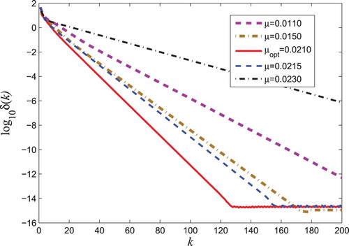
From Figure 1, it can be seen that the Algorithm 3.1 is convergent when the tunable parameter belongs to $0<\mu <$ $\mathrm{0.0239.}$ In addition, the optimal tuning parameter leads to the fastest convergence rate.

Simulation 2: In this simulation, we will compare the convergence performance of the proposed gradient-based iterative Algorithm 3.1 with some existing iterative Algorithms 2.1, 2.2, 2.3 and 2.4 in terms of computational time. By applying the method in [7], we choose the step size $\mu ={\mu }_{\mathrm{o}\mathrm{p}\mathrm{t}}=0.0214$ such that the Algorithm 2.3 with initial conditions (28(28) $\begin{array}{rl}{X}_1\left(0\right)& =\left[\begin{array}{ccc}1& 0& 0.5\\ 0& 0& 1.2\\ 2& -3& 0.8\end{array}\right],\\ X_2\left(0\right)& =\left[\begin{array}{ccc}-1& 0.5& 0.7\\ 1& 0& 0.9\\ 0& 2.1& -1\end{array}\right],\\ X_3\left(0\right)& =\left[\begin{array}{ccc}0.8& -0.5& 1.6\\ 0.15& 2.3& -0.7\\ 0.3& -2.1& 1.5\end{array}\right].\end{array}$(28) ) has the maximal convergence rate. For the Algorithm 2.4, the fastest convergence rate can be obtained when the step size is chosen as $\mu ={\mu }_{\mathrm{o}\mathrm{p}\mathrm{t}}=0.0161$. By using the method in Theorem 3.2, it can be derived that the Algorithm 3.1 has the best convergence performance if $\mu ={\mu }_{\mathrm{o}\mathrm{p}\mathrm{t}}=0.0210$. By using different iterative algorithms to solve the continuous CLMEs (3(3) $A_i^{\mathrm{T}}{X}_i+X_i{A}_i+\sum _{j=1}^N{\pi }_{ij}{X}_j+Q_i=0,i\in \mathbb{I}\mathbb{[}1,N\mathbb{]},$(3) ), thus we obtain the computational time and the iterative errors for different algorithms as shown in Table 1 for precision $\delta \left(k\right)\ge {10}^{-15}$.

From Table 1, one can see that the Algorithm 3.1 takes less computational time than the previous iterative Algorithms 2.1, 2.2, 2.3 and 2.4. In addition, the iteration errors ${\log }_{10}\delta \left(k\right)$ versus k for Algorithms 2.3, 2.4 and 3.1 are shown in Figure 2.

Figure 2. The convergence performance of the different gradient-based iterative algorithms.

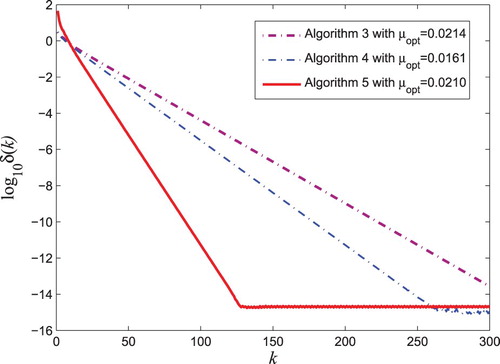
Table 1. Comparison of the convergence performance for different iterative algorithms.

Iterative algorithms	1	2	3	4	5
Computational time	0.031658 s	0.030869 s	0.001228 s	0.002507 s	0.000103 s

It can be seen from Figure 2 that the proposed Algorithm 3.1 is more effective and converge much faster than the previous gradient-based iterative Algorithms2.3 and 2.4. The total iterative numbers of the Algorithms2.3, 2.4 and 3.1 with a same cutoff error ${10}^{-14}$ are 300, 260 and 120, respectively. Thus, the convergence rate of the proposed Algorithm 3.1 is much faster than the existing Algorithms 2.3 and 2.4.

Example 4.2

In this paper, we show that effectiveness of the proposed gradient-based Algorithm for the continuous CLMEs (3(3) $A_i^{\mathrm{T}}{X}_i+X_i{A}_i+\sum _{j=1}^N{\pi }_{ij}{X}_j+Q_i=0,i\in \mathbb{I}\mathbb{[}1,N\mathbb{]},$(3) ) with high-dimensional system matrices. Consider the following continuous CLMEs in the form of (3(3) $A_i^{\mathrm{T}}{X}_i+X_i{A}_i+\sum _{j=1}^N{\pi }_{ij}{X}_j+Q_i=0,i\in \mathbb{I}\mathbb{[}1,N\mathbb{]},$(3) ) with N=2. The system matrices are as follows:

$\begin{array}{rl}{A}_1& =\left[\begin{array}{cccccccccc}-3.3313& -3.1173& -3.7911& -3.4597& -4.2978& -3.5612& -3.1514& -4.4412& -4.9275& -3.1113\\ -3.1173& -6.0572& -4.2081& -6.0757& -6.9933& -5.8278& -3.8478& -6.0925& -6.3057& -5.4731\\ -3.7911& -4.2081& -5.6183& -4.3528& -4.5035& -4.9983& -4.1194& -5.3772& -5.4906& -4.8210\\ -3.4597& -6.0757& -4.3528& -7.7505& -8.3844& -5.4953& -4.2787& -5.7269& -6.5043& -6.1859\\ -4.2978& -6.9933& -4.5035& -8.3844& -10.2603& -5.7841& -4.4345& -7.4483& -8.0805& -6.6060\\ -3.5612& -5.8278& -4.9983& -5.4953& -5.7841& -8.2986& -5.5146& -6.4328& -7.0797& -5.1943\\ -3.1514& -3.8478& -4.1194& -4.2787& -4.4345& -5.5146& -4.4088& -5.0494& -5.5947& -4.0898\\ -4.4412& -6.0925& -5.3772& -5.7269& -7.4483& -6.4328& -5.0494& -9.0362& -8.2483& -6.5311\\ -4.9275& -6.3057& -5.4906& -6.5043& -8.0805& -7.0797& -5.5947& -8.2483& -9.6603& -6.2078\\ -3.1113& -5.4731& -4.8210& -6.1859& -6.6060& -5.1943& -4.0898& -6.5311& -6.2078& -7.3382\end{array}\right],\\ A_2& =\left[\begin{array}{cccccccccc}-5.6400& -4.6558& -5.8251& -4.8026& -6.6079& -4.8687& -4.4065& -6.5460& -8.1805& -3.8238\\ -4.6558& -6.9513& -5.4297& -6.8532& -8.2161& -7.0980& -4.6756& -6.3913& -8.3178& -4.8481\\ -5.8251& -5.4297& -7.2981& -5.1086& -6.3680& -5.7261& -4.9133& -7.3166& -8.2418& -5.0372\\ -4.8026& -6.8532& -5.1086& -9.2468& -10.2573& -6.4203& -5.0568& -5.6261& -8.4116& -5.9118\\ -6.6079& -8.2161& -6.3680& -10.2573& -12.8308& -7.2576& -5.7195& -8.1378& -10.9120& -6.5402\\ -4.8687& -7.0980& -5.7261& -6.4203& -7.2576& -10.1240& -6.5006& -7.0499& -9.5459& -4.7922\\ -4.4065& -4.6756& -4.9133& -5.0568& -5.7195& -6.5006& -5.2548& -5.9297& -7.7278& -4.1116\\ -6.5460& -6.3913& -7.3166& -5.6261& -8.1378& -7.0499& -5.9297& -10.2524& -10.2895& -5.7193\\ -8.1805& -8.3178& -8.2418& -8.4116& -10.9120& -9.5459& -7.7278& -10.2895& -14.6022& -6.6714\\ -3.8238& -4.8481& -5.0372& -5.9118& -6.5402& -4.7922& -4.1116& -5.7193& -6.6714& -6.0503\end{array}\right],\end{array}$

and transition rate matrix is $\begin{array}{r}\mathrm{\Pi }=\left[\begin{array}{cc}-0.3& 0.3\\ 0.5& -0.5\end{array}\right].\end{array}$ In this example, the dimension of the above system is n=9 and the positive definite matrices $Q_i,i=1,2$ are both chosen as identity matrices. Next, the convergence performance of the different algorithms with the zero initial conditions. For this example, by applying the method in [7], we choose the step size $\mu ={\mu }_{\mathrm{o}\mathrm{p}\mathrm{t}}=0.0082$ such that the Algorithm 2.3 with initial conditions (28(28) $\begin{array}{rl}{X}_1\left(0\right)& =\left[\begin{array}{ccc}1& 0& 0.5\\ 0& 0& 1.2\\ 2& -3& 0.8\end{array}\right],\\ X_2\left(0\right)& =\left[\begin{array}{ccc}-1& 0.5& 0.7\\ 1& 0& 0.9\\ 0& 2.1& -1\end{array}\right],\\ X_3\left(0\right)& =\left[\begin{array}{ccc}0.8& -0.5& 1.6\\ 0.15& 2.3& -0.7\\ 0.3& -2.1& 1.5\end{array}\right].\end{array}$(28) ) has the maximal convergence rate. For the Algorithm2.4, the fastest convergence rate can be obtained when the step size is chosen as $\mu ={\mu }_{\mathrm{o}\mathrm{p}\mathrm{t}}=0.0051$. By using the method in Theorem 3.2, it can be derived that the Algorithm 3.1 has the best convergence performance if $\mu ={\mu }_{\mathrm{o}\mathrm{p}\mathrm{t}}=0.0069$.

First, the converge curves for Algorithms 2.3–3.1 are given in Figure 3.

Figure 3. The convergence performance of the different gradient-based iterative algorithms with high-dimensional system matrices.

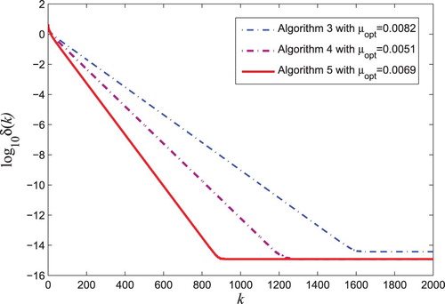
For the continuous CLMEs (3(3) $A_i^{\mathrm{T}}{X}_i+X_i{A}_i+\sum _{j=1}^N{\pi }_{ij}{X}_j+Q_i=0,i\in \mathbb{I}\mathbb{[}1,N\mathbb{]},$(3) ) with high-dimensional system matrices, it can be seen from Figure 3 that the proposed gradient-based Algorithm 3.1 with zero initial conditions has faster convergence rate than the previous Algorithms 2.3–2.4 if the tuning parameter is appropriately chosen.

For this example with high-dimensional system matrices, we next compare the proposed Algorithm 3.1 with the existing Algorithms 2.1–2.4 in terms of the computational time. By using different iterative algorithms to solve the coupled Lyapunov matrix Equation (3(3) $A_i^{\mathrm{T}}{X}_i+X_i{A}_i+\sum _{j=1}^N{\pi }_{ij}{X}_j+Q_i=0,i\in \mathbb{I}\mathbb{[}1,N\mathbb{]},$(3) ) with zero initial conditions, the computational time with the cutoff iterative errors $\delta ={10}^{-14}$ in the following table.

From Table 2, it can be seen that if the parameter μ is properly chosen, then the proposed gradient-based iterative Algorithm 3.1 takes less computational time than the existing Algorithms 2.1–2.4. From these results, it can be concluded that the proposed Algorithm 3.1 has much computational cost than the existing Algorithms 2.1–2.4 even if the coupled Lyapunov matrix Equation (3(3) $A_i^{\mathrm{T}}{X}_i+X_i{A}_i+\sum _{j=1}^N{\pi }_{ij}{X}_j+Q_i=0,i\in \mathbb{I}\mathbb{[}1,N\mathbb{]},$(3) ) has high-dimensional system matrices.

Table 2. Comparison of the convergence performance of the Algorithms 2.1–3.1 with high-dimensional system matrices.

Iterative algorithms	1	2	3	4	5
Computational time	0.110253 s	0.008419 s	0.003658 s	0.003019 s	0.002395 s

5. Conclusions

In this paper, a gradient-based iterative algorithm is given for solving the continuous CLMEs (3(3) $A_i^{\mathrm{T}}{X}_i+X_i{A}_i+\sum _{j=1}^N{\pi }_{ij}{X}_j+Q_i=0,i\in \mathbb{I}\mathbb{[}1,N\mathbb{]},$(3) ) which arises in the continuous-time Markovian jump linear systems.The structure of this new gradient-based iterative algorithm is much simpler than the existing gradient-based iterative algorithms. It has been proved that the sequence generated by the proposed algorithm converge to the unique positive definite solution of the continuous CLMEs (3(3) $A_i^{\mathrm{T}}{X}_i+X_i{A}_i+\sum _{j=1}^N{\pi }_{ij}{X}_j+Q_i=0,i\in \mathbb{I}\mathbb{[}1,N\mathbb{]},$(3) ) with faster convergence rates in comparison with existing algorithms. Moreover, the optimal tunable parameter achieving the fastest convergence rate is explicitly provided.

In future, it is expected that the ideas and methods can be further used to solve the other matrix equations such as coupled Riccati matrix equations, discrete coupled Lyapunov equations, etc.

Disclosure statement

No potential conflict of interest was reported by the authors.

Additional information

Funding

This work was supported by the National Natural Science Foundation of China [grant numbers31370565 and 51278227].

References

- Mariton M. Almost sure and moments stability of jump linear systems. Syst Control Lett. 1988;11(5):393–397. doi: 10.1016/0167-6911(88)90098-9
- Ji Y, Chizeck HJ. Controllability, stabilizability, and continuous-time Markovian jump linear quadratic control. IEEE Trans Automat Contr. 1990;35(7):777–788. doi: 10.1109/9.57016
- Sun HJ, Wu AG, Zhang Y. Stability and stabilisation of Ito stochastic systems with piecewise homogeneous Markov jumps. Int J Syst Sci. 2018;50(2):307–319. doi: 10.1080/00207721.2018.1551977
- Luo TJ. Stability analysis of stochastic pantograph multi-group models with dispersal driven by G-Brownian motion. Appl Math Comput. 2019;354:396–410.
- Jodar L, Mariton M. Explicit solutions for a system of coupled Lyapunov differential matrix equations. Proc Edinburgh Math Soc. 1987;30(2):427–434. doi: 10.1017/S0013091500026821
- Ge ZW, Ding F, Xu L. Gradient-based iterative identification method for multivariate equation-error autoregressive moving average systems using the decomposition technique. J Franklin Inst. 2019;356(3):1658–1676. doi: 10.1016/j.jfranklin.2018.12.002
- Zhang HM. Quasi gradient-based inversion-free iterative algorithm for solving a class of the nonlinear matrix equations. Comput Math Appl. 2019;77(5):1233–1244. doi: 10.1016/j.camwa.2018.11.006
- Zhang H. Reduced-rank gradient-based algorithms for generalized coupled Sylvester matrix equations and its applications. Comput Math Appl. 2015;70(8):2049–2062. doi: 10.1016/j.camwa.2015.08.013
- Ding F, Zhang H. Gradient-based iterative algorithm for a class of the coupled matrix equations related to control systems. IET Control Theory Appl. 2014;8(15):1588–1595. doi: 10.1049/iet-cta.2013.1044
- Hajarian M. On the convergence of conjugate direction algorithm for solving coupled Sylvester matrix equations. Comput Appl Math. 2018;37(3):3077–3092. doi: 10.1007/s40314-017-0497-y
- Sun HJ, Zhang Y, Fu YM. Accelerated Smith iterative algorithms for coupled Lyapunov matrix equations. J Franklin Inst. 2017;354(15):6877–6893. doi: 10.1016/j.jfranklin.2017.07.007
- Sun HJ, Liu W, Teng Y. Explicit iterative algorithms for solving coupled discrete-time Lyapunov matrix equations. Iet Control Theory Appl. 2016;10(18):2565–2573. doi: 10.1049/iet-cta.2016.0437
- Huang BH, Ma CF. Gradient-based iterative algorithms for generalized coupled Sylvester-conjugate matrix equations. Comput Math Appl. 2017;75(7):2295–2310. doi: 10.1016/j.camwa.2017.12.011
- Zhang H, Yin H. New proof of the gradient-based iterative algorithm for the Sylvester conjugate matrix equation. Comput Math Appl. 2017;74(12):3260–3270. doi: 10.1016/j.camwa.2017.08.017
- Borno I. Parallel computation of the solutions of coupled algebraic Lyapunov equations. Automatica. 1995;31(9):1345–1347. doi: 10.1016/0005-1098(95)00037-W
- Qian YY, Pang WJ. An implicit sequential algorithm for solving coupled Lyapunov equations of continuous-time Markovian jump systems. Automatica. 2015;60:245–250. doi: 10.1016/j.automatica.2015.07.011
- Wu AG, Duan GR, Liu W. Implicit iterative algorithms for continuous Markovian jump Lyapunov equations. IEEE Trans Automat Contr. 2016;61(10):3183–3189. doi: 10.1109/TAC.2015.2508884
- Wu AG, Sun HJ, Zhang Y. An SOR implicit iterative algorithm for coupled Lyapunov equations. Automatica. 2018;97:38–47. doi: 10.1016/j.automatica.2018.07.021
- Damm T, Sato K, Vierling A. Numerical solution of Lyapunov equations related to Markov jump linear systems. Numer Linear Algebra Appl. 2017;25(6):13–14.
- Hajarian M. Convergence properties of BCR method for generalized Sylvester matrix equation over generalized reflexive and anti-reflexive matrices. Linear Multilinear Algebra. 2018;66(10):1975–1990. doi: 10.1080/03081087.2017.1382441
- Zhang H. A finite iterative algorithm for solving the complex generalized coupled Sylvester matrix equations by using the linear operators. J Franklin Inst. 2017;354(4):1856–1874. doi: 10.1016/j.jfranklin.2016.12.011
- Tian ZL, Fan CM, Deng YJ, et al. New explicit iteration algorithms for solving coupled continuous Markovian jump Lyapunov matrix equations. J Franklin Inst. 2018;355(17):8346–8372. doi: 10.1016/j.jfranklin.2018.09.027
- Brewer J. Kronecker products and matrix calculus in system theory. IEEE Trans Circuits Syst. 1978;25(9):772–781. doi: 10.1109/TCS.1978.1084534