Optic disc localization using interference map and localized segmentation using grab cut

Abstract

Many eye diseases such as Diabetic Retinopathy, Cataract, Glaucoma have their symptoms shown in the retina. To detect such diseases, the normal and abnormal retina should be differentiated. The Optic disc has been a prominent landmark for finding abnormalities in the retina. In this paper, we attempted two methods to localize the optic disc using the segmentation which is done on the interference map that is obtained from a family of generalized motion patterns of the image. In brief, we are adding motion to the image so that the bright regions can be extracted well by improving the contrast between the object and its background in the image. Then, the region of interest has been taken and binary image has been generated. In the 1st method, by thresholding, the optic disc has been segmented and its centre has been found. In the second method, the grab cut is used for segmentation. Both of our methods show better results when compared with the competing method.

KEYWORDS:

• Thresholding
• segmentation
• optic disc
• optic disc centre
• grabcut
• graph cut

1 Introduction

Diabetic Retinopathy and Glaucoma are the most common diseases related to the retina. Detecting the abnormality and symptoms in the early stage can prevent or lessen the effect of vision loss. Most common computer-aided techniques need ophthalmologist’s examination and supervision on the diagnosis results. By providing information about the abnormalities, we are reducing the burden of the ophthalmologist. Thereby also helping a non-expert understand the problem. The efficiency of diagnosis can be improved by predicting the abnormalities more accurately.

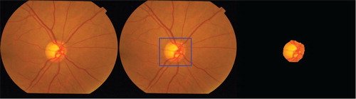
For the automated detection of the abnormality, the detection of the optic disc and macula assist us to get vital information. Many methods have been discussed in the literature for finding the optic disc by observing the intensity and geometrical features. In our work, we proposed two methods for segmenting the optic disc. The first method is an extension to [1] which uses Interference map introduced in [2] to segment the optic disc. We extended the concept by applying a threshold on the red channel image which proved to be more effective and efficient, based on the results we observed. The second method uses the graph cut method by using the prior information obtained from the [1] method (Figure 22). This graph cut based method has given even better results compared to the first method. In the following sections, we present a literature survey, give a rundown about the method we adopted and discuss the novelty we brought, followed by experimental study and conclusion.

2 Literature survey

Many optic disc segmentation methods have been proposed in the past. However, finding the exact optic disc centre and accurate segmentation is a challenging problem. A few thresholding based optic disc segmentation approaches proposed in the literature are summarized as follows.

The paper by Thomas et al. talks about using morphological techniques. The input image was filtered with a hexagonal shaped structuring element with closing and opening operations. Later thresholded to get the bright region which contains optic disc in the form of a binary image. Contours of the optic disc were obtained using gradient-based watershed transformation. However, the method was not efficient for the low contrast images and irregular illuminations [3].

The paper by Ghafar et al. talks about using hough transform to get some approximate optic disc. Lee filter was applied to attenuate the distortions. The input retinal image was firstly enhanced using Sobel operator and the local thresholding was applied using mean and variance. Later, the output obtained by using Hough transform and lee filter was thresholded to obtain the optic disc by taking the maximum intensity region [4].

The paper by Noor et al. talks about finding the cup to disc ratio for the diagnosis of glaucoma. The minimum, maximum and mean values from each red, red and green channels were considered for finding the multiple thresholds. Initially, the region of interest was taken. Later, post processing was applied to find the cup to disc ratio. But the performance of optic disc and optic cup segmentation were degraded [5].

The paper by Tehmina et al. talks about applying Otsu’s thresholding for the image. Image pre-processing was done using bi-linear interpolation and histogram equalization to enhance resolution and contrast. Later, the noise was removed using mean and median filters. Then, Otsu’s thresholding was applied to get the initial optic disc. At last, the convex hull was applied to the obtained output to get the ultimate optic disc [6].

3 GMP and interference map

3.1 Generalized motion pattern

The concept of Generalized motion pattern(GMP) was used in [7]. They argue that the smear pattern holds more information about the scene and simulated it by inducing motion in a given image. The resulting sequence of images are coalesced to form a motion pattern. Such GMP is given by (1) $\begin{array}{r}{I}_{\text{GMP}}\left(\overleftarrow{x}\right)=f(I(T_i\left(\overleftarrow{x}\right)|1\le i\le N))\end{array}$(1) where $\overleftarrow{x}$ denotes the pixel location and $i$ denotes the ith image obtained for applying ith rotation of the image forming $N$ images totally. $f(.)$ is the coalescing function applied on those images for obtaining the GMP.

3.2 Interference map

The K GMPs generated with K different pivots (randomly selected points in the image) are combined together to get an Interference Map [2]. Interference Map is given by (2) $\begin{array}{r}{I}_{\text{int}}\left(\overleftarrow{x}\right)=\phi (C_k)=\phi (I_{\text{GMP}}^k\left(\overleftarrow{x}\right)|1\le k\le K)\end{array}$(2) The coalescing function $\phi (.)$ combines all GMPs into an Interference Map. The method [1] uses this Interference Map to find the optic disc. 150 pivot points were chosen randomly and the image was rotated about the pivot point with step angle($\theta$) 1 within range $(0,360)$. Median was used as coalescing function $f(.)$ and pointwise quartile generator as $\phi (.)$. The interference map generated in this process gives the information about the bright regions in the image. The interference map is thresholded using (3) to give binary image which contains candidate regions. (3) $\begin{array}{rl}{I}_{\text{bin}}^j\left(\overleftarrow{x}\right)& =(\begin{array}{cc}255& \text{if}{I}_{\text{int}}\left(\overleftarrow{x}\right)>I_{\text{high}}-j\ast \mathrm{step}\mathrm{\_}\mathrm{size}\\ 0& \text{otherwise}\end{array}\end{array}$(3) (4) $\begin{array}{rl}\text{step\_size}& =(I_{\text{high}}-I_{\text{low}})/20\end{array}$(4) The time taken for the method [1] to segment OD is high as they are taking 150 pivot points. We observed that max interference map generation works better than the median interference map generation when tested with standard dataset Drishti-GS1 [8].

4 Grab cut Technique

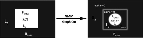
Grab cut [9] is an algorithm which is used widely for solving segmentation problems. It uses the Gaussian Mixture Model (GMM) to model the probability distribution over the pixels and trains it iteratively to segment the foreground and background regions by incorporating the graph cuts [10].

A graph is constructed as follows: $G=(V,E,C)$ where $V=P{\cup }^{\{}s,t\}$,

where $P=\{(i,j)/(i,j)$ is pixel location, $0\le i\le m-1,0\le j\le n-1\}$ s and t are special vertices called source and sink respectively.

$E=\{(u,v)/u,v\in P\text{and }u\text{ and }v\text{ are adjacent vertices}\}$ ${\cup }^{\{}(s,v)/v\in P\}{\cup }^{\{}(v,t)/v\in P\}$for each (u,v) $\in$ E, C(u,v) is defined using GMM as follows:

Two GMMs are created for background region and foreground region. Each one has $5$ clusters to cluster the RGB pixel values of the given image. The parameters of each gaussian cluster c are ${\mu }_c$, ${\mathrm{\Sigma }}_c$ and ${\pi }_c$. GMM is given by (5) $\begin{array}{r}p(x)={\mathrm{\Sigma }}_{c=1}^K{\pi }_c\mathcal{N}(x|{\mu }_c,{\mathrm{\Sigma }}_c)\end{array}$(5) where (6) $\begin{array}{rl}\mathcal{N}(x|\mu ,\mathrm{\Sigma })& =\frac{1}{{(2\pi )}^{D/2}}\frac{1}{|\mathrm{\Sigma }{|}^{1/2}}\\ & \times \text{exp}\{-\frac{1}{2}(x-\mu {)}^T{\mathrm{\Sigma }}^{-1}(x-\mu )\}\end{array}$(6)

The labels of background and foreground are given as ${\alpha }_n=0$ and ${\alpha }_n=1$. Initially, a trimap is used which is defined as $L=\{L_B,L_U,L_F\}$. Where $L_B$ is set of all background pixels, $L_U$ is set of all unknown pixels and $L_F$ is set of all foreground pixels. When the segmentation is initialized, the region around the rectangular box (ROI) is treated as a background region and stored in $L_B$. Pixel inside the rectangular box are stored in $L_U$ and $L_F$ will be an empty set.

The GMM for the background is created by the pixels in $L_B$ where ${\alpha }_n=0$ and the GMM for the foreground is created by the pixels in $L_U$ where ${\alpha }_n=1$. Iterations are performed by grab cut to assign the foreground and background labels and by clustering the pixels in $L_U$ depending on the weighting function defined as [11]: (7) $\begin{array}{rl}& C(s,n)=-\text{log}\sum _{c=1}^K\pi (1,c)\frac{1}{\sqrt{\det \mathrm{\Sigma }(1,c)}}\\ & e^{-\frac{1}{2}{[z_n-\mu (1,c)]}^T\mathrm{\Sigma }{(1,c)}^{-1}[z_n-\mu (1,c)]}\end{array}$(7) (8) $\begin{array}{rl}& C(t,n)=-\text{log}\sum _{c=1}^K\pi (0,c)\frac{1}{\sqrt{\det \mathrm{\Sigma }(0,c)}}\\ & e^{-\frac{1}{2}{[z_n-\mu (0,c)]}^T\mathrm{\Sigma }{(0,c)}^{-1}[z_n-\mu (0,c)]}\end{array}$(8) where $\pi (1,c)={\pi }_c$ given by GMM for foreground,

$\pi (0,c)={\pi }_c$ given by GMM for background,

$n$ $L_U$ and $z$ is RGB row vector for $n$

for each $n$ $\in$ $L_U$

$c_n:\text{arg min}{C}_n({\alpha }_n,c_n,{\mu }_n,{\mathrm{\Sigma }}_n,\pi \mathrm{\_}n,z_n)$ $c_n\in \{1,2,\dots ,K\}$

Let p,q be two neighbouring pixels in the image, the edge weight function for the edges between the neighbouring pixels is defined as $\text{C}\text{(}\text{p,q}\text{)}=\delta \text{(}{\alpha }_{\text{p}}\text{,}{\alpha }_{\text{q}}\text{)}{\text{e}}^{-}\beta \text{(}\parallel {\text{z}}_{\text{p}}-{\text{z}}_{\text{q}}\parallel {\text{)}}^{\text{2}}$

where $\beta =(2<({\text{z}}_{\text{p}}-{\text{z}}_{\text{q}}{\text{)}}^{\text{2}}{>)}^{-\text{1}}$ where <·> denotes the expectation over the image. and $\beta \text{(}\text{p,q}\text{)}=\begin{array}{cc}\text{1}& \text{if}{\alpha }_p\ne {\alpha }_q\\ \text{0}& \text{otherwise}\end{array}$

Once the graph is constructed, min cut is performed to segment foreground and background regions [9]. The Figure 1 shows the pipeline of the grabcut algorithm.

Figure 1 Pipeline of the Grab cut algorithm.

5 Proposed methods

5.1 Method 2

We adopted the method to crop the ROI from the red channel using less number of pivot points which reduces computational time by a significant margin. The ROI is of fixed size 500×500 pixels. We have experimented with different thresholds and found that below mentioned threshold was giving better results. Using the thresholding, (9) $\begin{array}{rl}{I}_{\text{OD}}\left(\overleftarrow{x}\right)& =(\begin{array}{lc}255& \text{if}{I}_{\text{ROI}}\left(\overleftarrow{x}\right)>(I_{\text{high}}-\text{range})\\ 0& \text{otherwise}\end{array}\end{array}$(9) (10) $\begin{array}{rl}\text{range}& =(I_{\text{high}}-I_{\text{low}})/2\end{array}$(10) the binary image is generated with a single candidate Optic disc region in 90% images in Drishti-GS1 dataset. Here $I_{\text{ROI}}$ in (Equation (9) denotes the region of interest (ROI) and $I_{\text{OD}}$ contains our candidate Optic discs in the form of a binary image. The centre of the largest candidate regions is found and considered as Optic disc centre. Our method produced better results compared to the method discussed in [1]. The proposed algorithm 1 is given in as follows.

ALGORITHM 1

Input: Fundus Image

Output: Segmented Optic disc and corresponding predicted Optic Centre.

1. Extract the Green channel of the input image $I_g$.

2. Using $I_g$ as an input, max interference map $I_{MP}$ is generated as discussed in [2].

3. Binary image is obtained from $I_{\text{MP}}$ by thresholding and centre of the candidate region in the binary image is calculated.

4. Consider in red channel, a square with fixed size $500\times 500$ whose centre is the centre obtained in S3.

5. Binary image of the ROI, I_OD is obtained through thresholding, which contains a single candidate region.

6. The centre of the candidate region in I_OD is considered as Optic Disc Centre and the candidate region is interfered to be Optic disc.

5.2 Method 2

We used the region of interest obtained from the adopted method as input to the grab cut algorithm [9]. It uses the prior information obtained from the region of interest which has foreground information as optic disc and the region outside the region of interest is treated as background region. It results the segmented optic disc region with a very good accuracy. We tested the algorithm with Drishti-GS1 dataset and got better results than our 1st method. The proposed algorithm 2 is given as follows:

ALGORITHM 2

Input: Fundus Image

Output: Segmented Optic disc.

1. Extract the Green channel of the input image $I_g$.

2. Using $I_g$ as an input, max interference map $I_{\text{MP}}$ is generated as discussed in [2].

3. Binary image is obtained from $I_{\text{MP}}$ by thresholding and centre of the candidate region in the binary image is calculated.

4. Consider a region of interest $ROI$ in RGB colour space about the centre obtained in S3.

5. The ROI is given as input to the grab cut algorithm

6. Binary image $I_{OD}$ is obtained as output of grab cut which contains a single candidate region.

7. The centre of the candidate region in $I_{OD}$ is considered as Optic disc Centre and the candidate region is interfered to be Optic disc.

6. Time complexity analysis

6.1. Method 1

The time taken to construct a GMP (I_GMP) is $\mathrm{\Theta }(mn\times N_{\theta })$ for an image of dimensions $m\times n$ where $N_{\theta }=360/\theta$. We are constructing an interference map (I_int) using K GMPs in S2. So the time taken for S2 is $\mathrm{\Theta }(mn\times N_{\theta }\times K)$. Rest all other steps take constant time. However, K and $N_{\theta }$ are kept as constants in practice. Therefore, the time complexity of the first method is $\mathrm{\Theta }(mn)$.

6.2. Method 2

The time taken to construct the graphs is $\mathrm{\Theta }(V+E)$ where $V$ is no. of vertices and $E$ is no. of edges. Assigning weights to the edges between pixels and terminal nodes uses GMM which runs EM algorithm to find the parameters in $\mathrm{\Theta }(Kmn)$ [12]. Here $K$ is no. of clusters in GMM which is kept as constant. The min cut/max flow algorithm takes $\mathrm{\Theta }(VE)$ [13].

Hence, the time taken for the extra work done in the second method is to find region of interest which takes $\mathrm{\Theta }(mn)+\mathrm{\Theta }(V+E)+\mathrm{\Theta }(Kmn)+\mathrm{\Theta }(VE)$.

Therefore, the time complexity of the 2nd method is $\mathrm{\Theta }(VE)$ where V is no. of vertices i.e. mn+2 and E is no. of edges.

7 Experiments and results

The proposed methods were evaluated on Drishti-GS1 [8] dataset, which has retinal images obtained from the subjects who are Indians. Figure 2 shows the soft map obtained on sample regions with Optic disc (OD) from the dataset. The later shows the OD centre obtained through our first approach for sample images from Drishti-GS1 dataset, which is marked with a cross in images of the last column (Figure 3). Figure 4 shows the Optic disc centre obtained from our first method for sample images from our dataset for which no Ground Truths(GT) are available. Despite intra-image variations, proposed method 1 produces very good estimates of the OD centre. The markings were uncertain for some images having irregular illuminations and noise. However, the method performs well as in most of the cases, the images are consistent in terms of illumination and colour intensities (Figure 5).

Figure 2. Softmap.

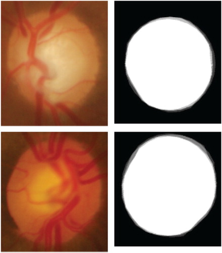
Figure 3. OD centre obtained by method 1 for images from Drishti dataset.

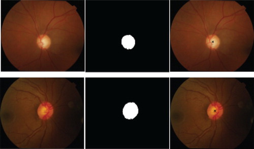
Figure 4. OD centre obtained by method 1 for images from private dataset.

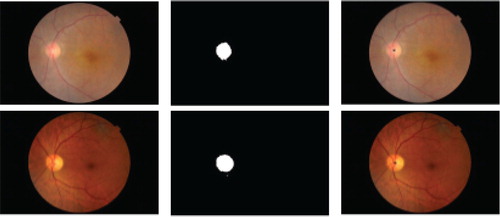
Figure 5. OD obtained by method 2 for images from Drishti dataset.

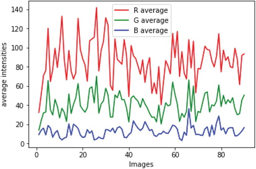
It has been observed that the red component of the image has been working well for segmenting the optic disc. The red channel of the retinal image has high pixel intensities compared to green and blue channels which can be seen in Figure 6. Where R average $(R_{\text{avg}})$, G average $(G_{\text{avg}})$ and B average $(B_{\text{avg}})$ are functions of number of images(image indices). Given by (10) $\begin{array}{rl}{R}_{\text{avg}}(k)& =\frac{\sum _{(x,y)}R(f_i)(x,y)}{mn}\end{array}$(10) (11) $\begin{array}{rl}{G}_{\text{avg}}(k)& =\frac{\sum _{(x,y)}G(f_i)(x,y)}{mn}\end{array}$(11) (12) $\begin{array}{rl}{B}_{\text{avg}}(k)& =\frac{\sum _{(x,y)}B(f_i)(x,y)}{mn}\end{array}$(12)

Figure 6. RGB plot.

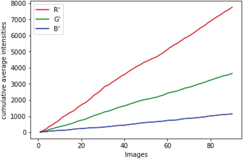
The cumulative averages have been obtained for the three channels which can be seen in Figure 7. The red channel grows rapidly with the increase in number of images when compared to other two channels. In Figure 7, $R^{\mathrm{\prime }}$, $G^{\mathrm{\prime }}$ and $B^{\mathrm{\prime }}$ are the functions of number of images given by (13) $\begin{array}{rl}R{}^{\mathrm{\prime }}(k)& =\sum _{i=1}^K\frac{\sum _{(x,y)}R(f_i)(x,y)}{mn}\end{array}$(13) (14) $\begin{array}{rl}G{}^{\mathrm{\prime }}(k)& =\sum _{i=1}^K\frac{\sum _{(x,y)}G(f_i)(x,y)}{mn}\end{array}$(14) (15) $\begin{array}{rl}B{}^{\mathrm{\prime }}(k)& =\sum _{i=1}^K\frac{\sum _{(x,y)}B(f_i)(x,y)}{mn}\end{array}$(15)

Figure 7. Cumulative RGB.

Where $R(f_i)(x,y)$ is the red component of the image $f_i$ at the location (x,y), $G(f_i)(x,y)$ is the green component of the image $f_i$ at the location (x,y) and $B(f_i)(x,y)$ is the blue component of the image $f_i$ at the location (x,y).

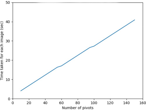
We studied the effect of the parameter setting on K, the number of pivot points. Greater the value K, more the evidence gathered in I_int at an increased computational cost (Figure 8). From Figure 9, we can observe that the time taken to perform the proposed method for a single image increases linearly with the number of pivots. According to [1], the evidence comprises of one or more bright regions, among which one serves as Optic disc. In both of our methods, we use the evidence gathered to locate the Optic disc region and use it as our ROI, so our approaches work fine even for less number of pivots. A high step angle (θ) affects localization while a low θ cannot soften out the background tissues.

Figure 8. Results obtained for different images after varying contrast.

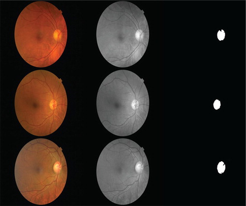
Figure 9. Relationship b/w no. of pivots and time taken.

R is the average of the radius of the optic discs for which GT is provided in Drishti-GS1. The accuracy is calculated based on the occurrence of predicted OD centre from the GT within a certain distance. Figure 10 shows the effect of varying k with θ=10 and distance is R/4. The plots indicate that for $35\le k\le 50$, better results are obtained. If the distance between the predicted OD centre and GT OD centre is less than $R/4$, then it is marked as correct prediction and the corresponding accuracy on the dataset are given in the second column of the Table 1. $\theta$ was assigned its optimal value (i.e,. 10). Similarly $R/2$ is considered and tabulated in the third column. The third and fourth columns of the Table 1 provide the information about Dice similarity coefficient (DSC) and Jaccard similarity coefficient (JSC) calculated using the below formula. (16) $\begin{array}{rl}\text{Accuracy}& =\frac{\text{TP}+\text{TN}}{\text{TP}+\text{FP}+\text{TN}+\text{FN}}\end{array}$(16) (17) $\begin{array}{rl}\text{Precision}& =\frac{\text{TP}}{\text{TP}+\text{FP}}\end{array}$(17) (18) $\begin{array}{rl}\text{Recall}& =\frac{\text{TP}}{\text{TP}+\text{FN}}\end{array}$(18) (19) $\begin{array}{rl}\text{DSC}& =\frac{2\times \mathrm{TP}}{2\times \mathrm{TP}+\mathrm{FP}+\mathrm{FN}}\end{array}$(19) (20) $\begin{array}{rl}\text{JSC}& =\frac{\text{TP}}{\text{TP + FP + FN}}\end{array}$(20)

Figure 10. Accuracy plot w.r.t no. of pivots.

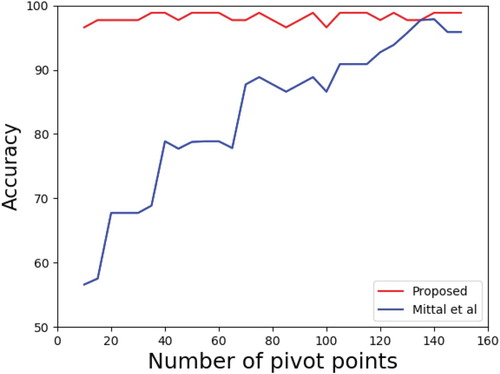
Table 1. Results of OD centres.

Method	R/4	R/2	DSC	JSC
Proposed method 1	90.01%	97.21%	0.925	0.992
Proposed method 2	92.22%	97.78%	0.934	0.993
Mittal et al.[1]	82.02%	94.38%	0.855	0.892

*R – Average OD radius.

True Positive (TP) contains the number of pixels that are commonly marked as OD in GT and prediction. False Positive (FP) contains the number of pixels that are falsely predicted as OD. False Negative (FN) contains the number of pixels that are falsely predicted as non-OD.

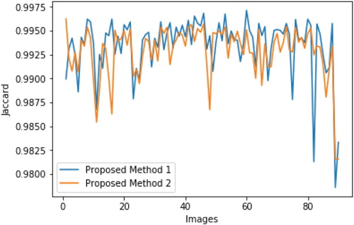
Figure 11 shows the Optic disc centre obtained from our second method for sample images from our dataset for which no Ground Truths(GT) are available. We compared the second method with first one which gave significant results for the Drishti-GS1 dataset which can be seen in Figure 12. In Figure 12 the images are in the X-axis and their respective Dice Similarity coefficients on Y-axis. In Figure 13 the images are in the X-axis and their respective Jaccard Similarity coefficients on Y-axis. Despite the variations in contrast obtained through contrast stretching, the proposed method 2 segmented the optic disc well which can be seen in the images 8 in the order of original, contrast stretched and optic disc segmented.

Figure 11. OD obtained by method 2 for images from private dataset.

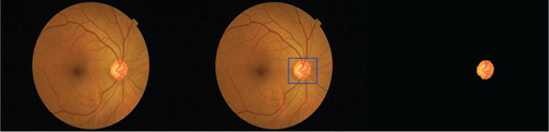
Figure 12. DSC Results.

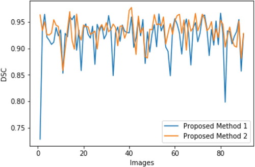
Figure 13. Jaccard Results.

Two methods have been tested on images with different Gaussian noise levels. It has been observed that, the second method performs well despite the noise in the images whereas first method was not producing the results. In Figure 14, the plot shows the performance of the second method with different standard deviations of the Gaussian noise on the X-axis and the Dice Similarity Coefficient (DSC) on the Y-axis. The Dice Similarity coefficient of 0.92 was obtained for the standard deviation of 10 which is a good result despite the noise. In Figure 15, the plot shows the performance of the second method with different standard deviations of the gaussian noise on the X-axis and the Jaccard Coefficients (JC) on the Y-axis. The Jaccard coefficient was also not affected much with an increase in noise levels.

Figure 14. DSC Noise Results.

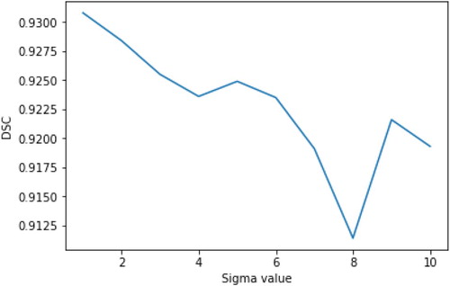
Figure 15. Jaccard Noise Results.

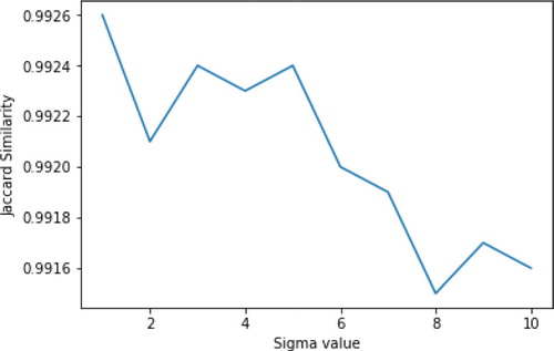
Figure 16. Segmentation accuracy for method 2.

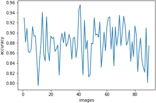
Figure 17. Segmentation precision for method 2.

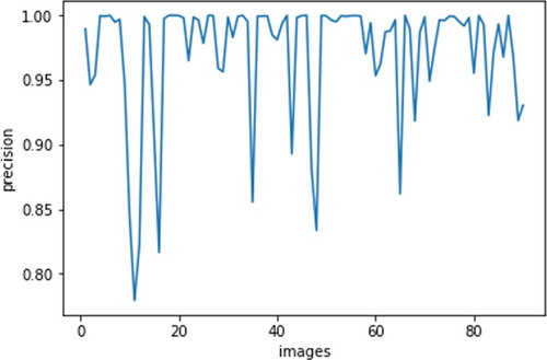
Figure 18. Segmentation recall for method 2.

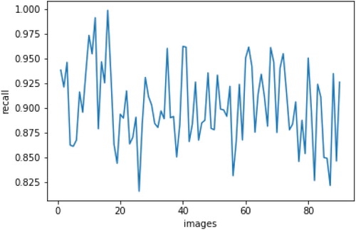
The precision, recall and accuracy for the segmentation have been obtained for both the proposed methods which can be seen in Table 2. The second method has outperformed the first method in terms of all metrics namely accuracy, precision and recall. The Figure 16 gives the performance of the second method where the image numbers(indices) are in X-axis and respective accuracy on the Y-axis. The Figure 17 gives the performance of the second method where the image numbers(indices) are in X-axis and respective precision on the Y-axis. The Figure 18 gives the performance of the second method where the image numbers(indices) are in X-axis and respective recall on the Y-axis. The Figure 19 gives the performance of both the methods where the image numbers(indices) are in X-axis and respective accuracy on the Y-axis. The Figure 20 gives the performance of both the methods where the image numbers(indices) are in X-axis and respective precision on the Y-axis. The Figure 21 gives the performance of both the methods where the image numbers(indices) are in X-axis and respective recall on the Y-axis.

Figure 19. Segmentation accuracy.

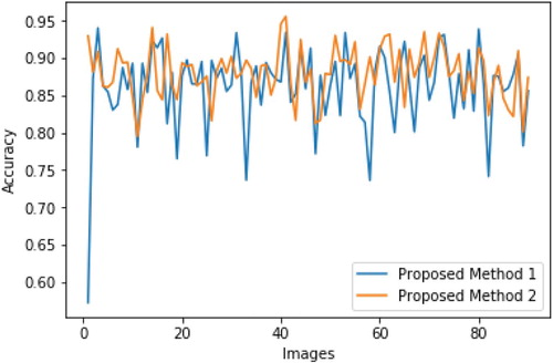
Figure 20. Segmentation precision.

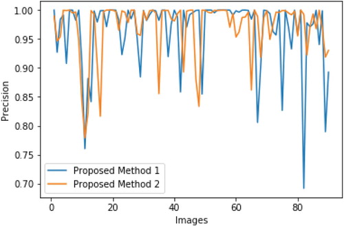
Figure 21. Segmentation recall.

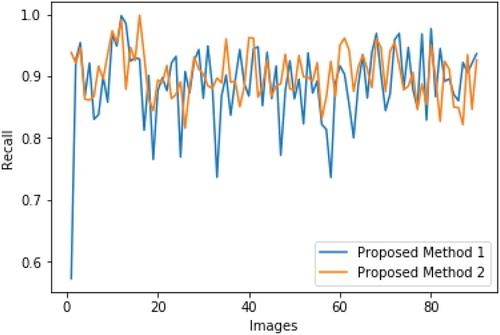
Figure 22. Pipeline of the proposed approaches.

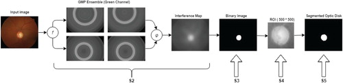
Table 2. Results of Segmentation.

Method	Precision	Recall	Accuracy
Proposed method 1	0.96	0.88	0.86
Proposed method 2	0.97	0.90	0.88

7 Conclusion

Two improvized methods of segmenting the optic disc have been implemented and improvement has been obtained because of localized segmentation. Applying motion to the object in the fundus image results in good contrast between optic disc and its background. Although the proposed method 1 gives good results in terms of efficiency and less time consuming compared to the competing method, its performance reduces in the case of irregularly illuminated images. The proposed method 2 uses iterative graph cuts and it is outperforming competing methods on the benchmark dataset Drishti-GS1 [8] and it also found to be robust to the gaussian noise. The manual intervening for graph cut segmentation has been eliminated by using the motion models. To make it a real-time process, the number of pivot points used is minimized without affecting the efficiency. Applying motions to the image has been working well to find the bright regions and can be extended further to find the abnormalities in the retina (Figure 22).

Disclosure statement

No potential conflict of interest was reported by the author(s).

References

- Mittal G, Sivaswamy J. Optic disk and macula detection from retinal images using generalized motion pattern. In 2015 Fifth National Conference on Computer Vision, Pattern Recognition, Image Processing and Graphics (NCVPRIPG), IEEE; 2015. p 1–4.
- Chakravarty A, Sivaswamy J, et al. An assistive annotation system for retinal images. In 2015 IEEE 12th International Symposium on Biomedical Imaging (ISBI), IEEE; 2015. p. 1506–1509.
- Walter T, Klein J-C. Segmentation of color fundus images of the human retina: Detection of the optic disc and the vascular tree using morphological techniques. In International Symposium on Medical Data Analysis, Springer; 2001, p. 282–287.
- Abdel-Ghafar RA, Morris T. Progress towards automated detection and characterization of the optic disc in glaucoma and diabetic retinopathy. Med Inform Internet Med. 2007;32(1):19–25. doi: 10.1080/14639230601095865
- Noor NM, Abdul Khalid NE, Md Ariff N. Optic cup and disc color channel multi-thresholding segmentation. In 2013 IEEE International Conference on Control System, Computing and Engineering, IEEE; 2013, p. 530–534.
- Khalil T, Akram MU, Khalid S, et al. Improved automated detection of glaucoma from fundus image using hybrid structural and textural features. IET Image Proc. 2017;11(9):693–700. doi: 10.1049/iet-ipr.2016.0812
- Sai Deepak K, Sivaswamy J. Automatic assessment of macular edema from color retinal images. IEEE Trans Med Imaging. 2012;31(3):766–776. doi: 10.1109/TMI.2011.2178856
- Sivaswamy J, Krishnadas S, Chakravarty A, et al. A comprehensive retinal image dataset for the assessment of glaucoma from the optic nerve head analysis. JSM Biomedical Imaging Data Papers. 2015;2(1):1004.
- Rother C, Kolmogorov V, Blake A. Grabcut: Interactive foreground extraction using iterated graph cuts. In ACM transactions on graphics (TOG), ACM; 2004. Vol 23, p. 309–314.
- Boykov YY and Jolly M-P. Interactive graph cuts for optimal boundary & region segmentation of objects in nd images. In Proceedings Eighth IEEE International Conference on Computer Vision, ICCV 2001, IEEE; 2001. Vol 1, p. 105–112.
- Talbot JF, Xu X. Implementing grabcut. Brigham Young University, 3, 2006.
- Verbeek JJ, Vlassis N, Kröse B. Efficient greedy learning of Gaussian mixture models. Neural Comput. 2003;15(2):469–485. doi: 10.1162/089976603762553004
- Orlin JB. Max flows in o (nm) time, or better. In Proceedings of the Forty-Fifth Annual ACM Symposium on Theory of Computing, ACM; 2013. p. 765–774.