Design of suboptimal model-matching controllers using squared magnitude function for MIMO linear systems

Abstract

This paper proposes a novel two-stage method for the design of a suboptimal model-matching controller in an output feedback closed-loop system (OFCLS) using the concept of squared magnitude function (SMF). A streamlined procedure for selection of a reference model, based on a linear quadratic regulator (LQR) with integral action (LQRI) having optimum values for the elements of the weighting matrices and the degree of interaction is proposed. The degrees of the numerator and denominator polynomials of the elements of the OFCLS transfer function matrix (TFM) are obtained from those of the plant and the chosen controller structure. In the first stage of the controller design, taking the LQRI-based closed-loop system (LCLS) as a reference model, the OFCLS is obtained using the approximate model-matching (AMM) technique based on the SMF concept. The approximation method involves a higher-order approximation for stable multiple-input-multiple-output (MIMO) lower-order systems. In the second stage, controller parameters are obtained using the exact model-matching (EMM) method with information about the OFCLS and plant TFMs. The proposed controller design method outperforms the method presented in the literature on integral squared error index. The simulation and experimental results illustrate the effectiveness of the proposed method.

KEYWORDS:

• Approximate model-matching
• exact model-matching
• interaction
• MIMO system
• squared magnitude function
• suboptimal controller

1. Introduction

The design of controllers for plants with interaction has been one of the challenges faced by researchers in the area of multiple-input-multiple-output (MIMO) control systems. The model-matching technique has been a powerful methodology for controller design of MIMO systems [1–9]. Controllers designed using the model-matching technique have been utilized for rejection of various types of disturbances [4]. The concepts of exact model-matching (EMM) of two-dimensional systems using state feedback have been described in [5]. The proposed methodology in [5] can be utilized for the design of two-dimensional filters. A centralized control strategy based on the equivalent transfer function (TF) is presented in [10]. An output feedback-based controller design methodology for higher-order SISO plants is presented in [11]. The methodology in [11] applies to unstable plant TFs. Model order reduction reduce the complexity of implementation of higher integer-order systems [12,13]. A model-order reduction method has been applied to closed-loop systems with parameter variations [14]. An algorithm for the design of controllers in multivariable systems using the approximate model-matching (AMM) technique has been proposed in [15,16]. EMM of linear time-varying multivariable systems was presented in [17]. A novel EMM methodology for generalized state-space systems via pure proportional state and output feedback was proposed in [18]. EMM has been solved using a generalization of Wolovich’s theorem [19]. The model-matching concept was used earlier for obtaining controllers for tracking and disturbances. In the present work, the AMM technique has been used for obtaining the output feedback closed-loop system (OFCLS) transfer function matrix (TFM), and in a following step, the controller TFM was obtained using the EMM technique.

Trajectory tracking has been achieved successfully using PID controllers in different types of systems [20,21]. Robust adaptive tracking control has been proposed for a nonholonomic mobile manipulator under system parameter uncertainties and external disturbances [22,23]. Trajectory tracking using linear quadratic regulator (LQR) techniques has been successfully applied to different types of systems [24,25]. The weighting matrices of the LQR controller have been determined using a genetic algorithm (GA) [26], particle swarm optimization [27] and pole placement [28]. The methods of determining of weighting matrices described in the literature have not considered the interactions present in MIMO systems. Interaction, as a specification to be preserved in the designed closed-loop system, i.e., OFCLS, has also been considered in the present work. The selection of reference model proposed in this work focuses on obtaining the optimal interaction factor for given desired output time-domain specifications together with finding the optimum main diagonal elements of the diagonal weighting matrices to be used in the LQR with an integral action (LQRI)-based closed-loop system (LCLS) design procedure. In the present work, the off-diagonal elements of a reference model TFM are determined by considering the optimum interaction present in the controlled system.

Squared magnitude continued fraction and factorization techniques are utilized to derive the stability-preserved reduced-order approximant [29]. A squared magnitude function (SMF)-based approach has been utilized in the approximation [30] and hardware implementation [31] of single-input-single-output (SISO) fractional-order systems. The retention of stability and minimum-phase characteristics has been achieved in model-order reduction of SISO linear systems using the concept of SMF [32]. The model-order reductions of SISO and MIMO systems have been solved using the method of integration of the stability equation together with the Padé approximation method [33]. The concept of SMF in the field of approximation yields a stable approximant. In the literature, the concept of SMF has been used for obtaining an approximation of SISO fractional-order systems or higher integer-order systems. The present work uses the AMM technique based on the concept of SMF to obtain a higher-order OFCLS representation, subsequently yielding controller parameters.

In the model-matching techniques reported in the literature, optimum interactions present in the OFCLS have not been considered. In [34], the authors developed an algorithm to obtain the desired interaction for a given degree of coupling. In the present work, the design procedure for obtaining a reference model incorporates the time-domain specifications and optimal interaction utilizing a simultaneous GA-based optimization procedure.

The rest of this paper is organized as follows. Section 2 presents the problem statement. The proposed method for selection of the reference model is described in Section 3. Section 4 details the proposed AMM algorithm based on the SMF concept. Section 5 describes the procedure to determine the controller parameters based on the EMM technique. Simulation and experimental results are provided in Sections 6 and 7 respectively. Finally, the concluding remarks and future scope are included in Section 8.

2. Statement of the problem

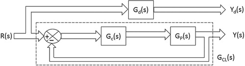
The objective of the present work is to design a controller G_c(s) for a MIMO plant G_P(s) using the model-matching technique. The controller design aims to make the response y(t) of the OFCLS G_CL(s) as close as possible to the response y_d(t) of the reference model G_d(s). G_d(s) is chosen in such a way that it reflects the desired closed-loop system characteristics, such as the desired time-domain specifications and the optimal interaction to be present in the G_CL(s). Model-matching controller design in the literature usually deals only with one of the two types of model-matching, namely EMM and AMM. The present work deals with both of these model-matching techniques for the design of G_c(s), thereby combining the advantages of both types into one algorithm. The important aspect of the controller design in the design and implementation is that the controller structure need not be fixed. The user can choose any controller structure to achieve the objectives. In addition, the solution for the controller parameters need not be unique. Certain controller parameters can be chosen, and the remaining controller parameters can be obtained according to the developed algorithm, resulting in a reduction in hardware compulsion. The present work leads to the retention of the stability property of the G_d(s) in the G_CL(s), thereby yielding a stabilizing G_c(s) in the second stage of the algorithm. The block diagrams of the reference model (LCLS model/user-defined model) and the OFCLS are shown in Figure 1.

Figure 1. Block diagram of desired and designed closed-loop system.

The plant can be represented in the s-domain as (1) $G_P(s)=\left[G_P^{(i,k)}(s)\right]=\frac{1}{d_P(s)}\left[n_P^{(i,k)}(s)\right]$(1) where $G_P^{(i,k)}(s)$, $i=1,2,\dots ,p;k=1,2,\dots ,q$ represents the elements of the plant TFM relating the kth input to the ith output. The numerator and denominator polynomials of each element of the plant TFM are represented by $n_P^{(i,k)}(s)$ and d_P(s) respectively.

The problem of finding G_c(s) such that G_CL(s) yields the same response as that of G_d(s) can be stated as follows. Find G_c(s) for the given MIMO plant from the information about the degrees of the numerator and denominator polynomials of elements of G_c(s) with the objective of obtaining the optimal interaction and specified time-domain specification in G_CL(s). In the proposed method for controller design, the first stage consists of an approximation of G_d(s) to a higher-order TFM G_CL(s). The degrees of the numerator and denominator polynomials of each element of G_CL(s) are obtained from those of the plant and the chosen controller structure (see Appendix A). In the second stage of the proposed method, G_c(s) is obtained by using the concept of EMM with the knowledge of G_P(s) and G_CL(s).

3. Reference model selection

This section proposes a streamlined procedure for the selection of G_d(s) which reflects the optimum degree of interaction and embodies the desired time-domain specifications.

3.1. Conventional model selection approach

Methods based on the preservation of the pole-zero excess of the plant [2] and specified time-domain specifications [34] have previously been utilized for G_d(s) selection. The approach presented in [34] embodies a specified interaction in the off-diagonal elements of the G_d(s) TFM. The limitation of the G_d(s) selection approaches presented in the literature is that they do not include information about the plant dynamics.

3.2. Proposed model selection procedure

The proposed method uses the LCLS model as G_d(s) for the design of G_c(s). The method uses an initial model which is utilized to compute the LCLS model. The initial model is framed with the desired time-domain specifications. The interaction parameters λ^(i,k) of the initial model are retained as tuning parameters. The LCLS model is framed by tuning the elements of the weighting matrices Q and R in the optimal state feedback design procedure. The interaction thus developed in the LCLS model is mapped onto the initial model by tuning the parameters λ^(i,k). The desired time-domain specifications of the initial model are used to tune the elements of the weighting matrices of the LCLS model. Thus, the LCLS model reflects the desired time-domain specifications and the optimal interaction to be present in G_CL(s).

3.2.1. Initial model

The desired transient response specifications include natural frequency, settling time, damping factor, etc. The initial model dynamics can be expressed in the form of TFM as (2) $[Y_m^{(i)}(s){]}_{{}_{p\times 1}}=G_m(s)[R_k(s){]}_{q\times 1}$(2) where $G_m(s)=[G_m^{(i,k)}(s)]$. Here, each $G_m^{(i,k)}(s)$, $i=1,2,\dots ,p;k=1,2,\dots ,q$ represents an element of the initial model TFM relating the ith output to the kth input. The Laplace transform of the desired responses is denoted by $Y_m^{(i)}(s)$, with steady-state values denoted by S_i. The desired profiles of $Y_m^{(i)}(s)$ can be taken in the form of the response of a standard second-order low-pass filter for R_i(s), taken as a step signal of amplitude S_i, i.e., (3) $Y_m^{(i)}(s)=\frac{{\text{S}}_{\text{i}}{\omega }_n^2}{s(s^2+2\zeta {\omega }_{n}s+{\omega }_n^2)}$(3) where ω_n is the natural frequency and ζ is the damping ratio, both of which can be determined from the desired time-domain specifications such as settling time, overshoot, rise time, etc. The (i,k)th off-diagonal elements of the initial model TFM are designed to have a pole at s = −λ^(i,k) and zero at s = ∞, which is utilized along with Equation (3) in Equation (2) to yield the expressions for diagonal elements of the initial model: (4) $\begin{array}{rl}{G}_m^{(u,u)}(s)& =\frac{\left(s{y}_m^{(u)}(s)-\sum _{\genfrac{}{}{0ex}{}{\mathrm{\forall }k}{k\ne u}}\frac{S_k}{(s+{\lambda }^{(u,k)})}\right)}{S_u}\end{array}$(4) where u = 1, 2, … , min(p,q); k = 1, 2, … , q.

For a given desired time-domain specification, the dynamics of G_m(s) will be a function of the parameter λ^(i,k). A given value of λ^(i,k) quantifies the interaction that can be present in the controlled dynamics. Higher values of λ^(i,k) imply a system with lesser interactions and vice versa. In the present work, a method of obtaining the optimized value of λ^(i,k) along with optimized values of the elements of the weighting matrices, is presented in subsection 3.2.3.

3.2.2. LCLS model

To eliminate the steady-state error, the integrating controller has full state feedback incorporated. The difference between the reference input and the output is integrated and the outputs of the integrators are considered as additional states. The combined structure is as given in [35].

In the combined structure, $x\in {\mathbb{R}}^{n\times 1}$, $u\in {\mathbb{R}}^{q\times 1}$, $y,x_i,r\in {\mathbb{R}}^{p\times 1}$ are the state, input, output, additional state and reference vectors respectively. The numbers of inputs, outputs and states present in the plant dynamic model are denoted by q, p and n respectively. The state-space representation of the plant G_P(s) shown in Equation (1) can be given as (5) $\dot{x}=Ax+Bu,\text{and}y=Cx,$(5) where the constant matrices $A\in {\mathbb{R}}^{n\times n},B\in {\mathbb{R}}^{n\times q},C\in {\mathbb{R}}^{p\times n}$, $K\in {\mathbb{R}}^{q\times n}$, and $K_i\in {\mathbb{R}}^{q\times p}$ are the state, input, output, state feedback gain and integral gain matrices respectively. Elimination of steady-state offset is achieved by incorporation of the integrator into the controlled system [35]. The overall TFM representing the LCLS model can be obtained by (6) $G_d(s)=C_{ag}(s{I}_{(n+p)}-(A_{ag}-B_{ag}{K}_{op}){)}^{-1}E$(6) where the optimal state feedback gain matrix is given by $K_{op}=-[K{K}_i]$, $K_{op}\in {\mathbb{R}}^{q\times (n+p)}$, $A_{ag}=\left[\begin{array}{cc}A& O_{n\times p}\\ -C& O_{p\times p}\end{array}\right],B_{ag}=\left[\begin{array}{c}B\\ O_{p\times q}\end{array}\right],$ C_ag = [$C{O}_{p\times p}$] and $E=\left[\begin{array}{c}{O}_{n\times p}\\ I_p\end{array}\right]$.

K_op is obtained by solving the algebraic Riccati equation for a given weighting matrices Q and R [25,26]. In the present work, the weighting matrices are obtained using the optimization procedure explained in the following subsection.

3.2.3. Weighting matrices and degree of interaction

The set of optimal weighting matrices and the degree of interaction have been determined by minimizing the difference in step response of G_m(s) and G_d(s). In the present work, the weighting matrices Q and R of the LQRI are assumed to be diagonal matrices. Hence, the aim of the optimization process is defined as follows.

Find the main diagonal elements of diagonal weighting matrices of LQRI and the off-diagonal pole location of the initial model TFM to

minimize (7) $\begin{array}{rl}{J}_1& =\sum _{i=1}^p(\sum _{k=1}^q(\sum _{\alpha =0}^{\tau }[{(y_m^{(i,k)}(\alpha \mathrm{\Delta }t)-y_d^{(i,k)}(\alpha \mathrm{\Delta }t))}^T\\ & \phantom{\sum _{i=1}^p(\sum _{k=1}^q(\sum _{\alpha =0}^{\tau }[{(y_m^{(i,k)}(\alpha \mathrm{\Delta }t)-y_d^{(i,k)}(\alpha \mathrm{\Delta }t))}^T}(y_m^{(i,k)}(\alpha \mathrm{\Delta }t)-y_d^{(i,k)}(\alpha \mathrm{\Delta }t))]))\end{array}$(7) subject to the constraints that the weighting matrices Q and R should be positive semi-definite, and positive definite matrices, respectively.

where the step responses of TFs relating the ith output to the kth input of G_m(s) and G_d(s) are represented by $y_m^{(i,k)}(\cdot )$ and $y_d^{(i,k)}(\cdot )$ respectively. The sample time and final time for the evaluation of the step response are $\mathrm{\Delta }t$ and $\tau \mathrm{\Delta }t$ respectively. The superscript T denotes the transpose of the matrix.

The solution of the optimization problem leads to an optimized value of λ^(i,k) and optimized values of the elements of the weighting matrices. The selection of the LCLS model over the initial model for G_d(s) as an input to the first stage of the proposed model-matching-based controller design procedure guarantees two major advantages. Firstly, the LCLS model is formulated by considering the dynamics of the plant. Secondly, the degrees of the numerator and denominator polynomials of elements of the LCLS model TFM will be closer to those of the OFCLS TFM in comparison to those of initial model TFM. The overall procedure for obtaining the optimal LCLS model from the information in the initial model can be illustrated in the form of a flow diagram as shown in Figure 2.

Figure 2. Flow diagram of the proposed reference model selection procedure.

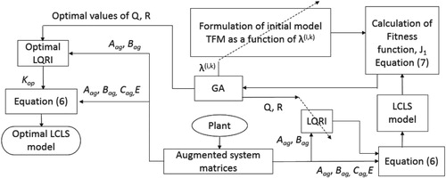
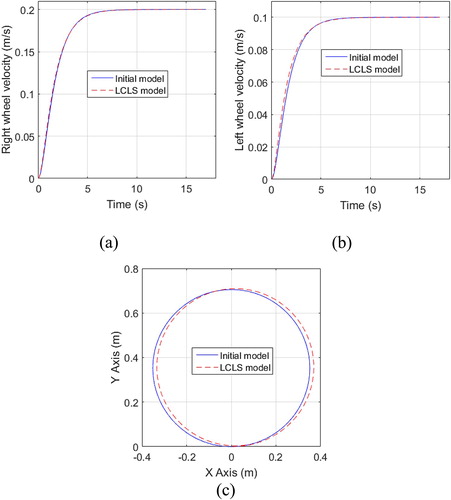
Figure 3. (a) Right wheel velocity profile. (b) Left wheel velocity profile. (c) The circular trajectory.

4. AMM technique based on SMF concept

This section presents the development of the proposed approximation algorithm for MIMO systems based on the concept of SMF. As part of the first stage of the proposed algorithm, an LCLS model TFM is approximated to the OFCLS TFM using SMF. If the degrees of the numerator and denominator polynomials of elements of the LCLS model TFM are same as those of the OFCLS TFM, the G_c(s) parameters may be obtained directly using EMM by taking the LCLS model itself as the OFCLS. In all other cases, the SMF-based approximation plays a role in the determination of OFCLS TFM.

4.1. Formulation of non-homogeneous simultaneous equations

This section describes the procedure for constructing non-homogeneous simultaneous equations, which are solved with the objective of finding parameters of SMF of OFCLS. Let G_d(s), obtained in the form of TFM via Equation (6), be expressed as (8) $G_d(s)=\left[G_d^{(i,k)}(s)\right]$(8) where $G_d^{(i,k)}(s)$, $i=1,2,\dots ,p;k=1,2,\dots ,q$ represents the elements of the G_d(s) TFM relating the kth input to the ith output. Elements of the TFM of G_d(s) can be represented as (9) $G_d^{(i,k)}(s)=\frac{a_0^{(i,k)}+a_1^{(i,k)}s+a_2^{(i,k)}{s}^2+\cdots +a_{m_1^{(i,k)}}^{(i,k)}{s}^{m_1^{(i,k)}}}{b_0+b_{1}s+b_2{s}^2+\cdots +b_{n_1}{s}^{n_1}}$(9) where $a_{\alpha }^{(i,k)}$, $\alpha =0,1,\dots ,m_1^{(i,k)}$ and $b_{\beta }$, $\beta =0,1,\dots ,n_1$ are the numerator and denominator polynomial coefficients of the (i,k)th element of the LCLS model TFM respectively, having $m_1^{(i,k)}\le n_1$. G_d(s) is to be approximated to a higher-order OFCLS TFM G_CL(s). Let G_CL(s) be represented in TF domain as (10) $G_{CL}(s)=\left[G_{CL}^{(i,k)}(s)\right]=\frac{1}{d_{CL}(s)}\left[n_{CL}^{(i,k)}(s)\right]$(10) where $G_{CL}^{(i,k)}(s)$, $i=1,2,\dots ,p;k=1,2,\dots ,q$, represents the elements of OFCLS TFM relating the kth input to the ith output. The numerator and denominator polynomials of each element of the OFCLS TFM are represented by $n_{CL}^{(i,k)}(s)$ and d_CL(s), respectively. Each element of the OFCLS TFM can be represented as (11) $G_{CL}^{(i,k)}(s)=\frac{d_0^{(i,k)}+d_1^{(i,k)}s+d_2^{(i,k)}{s}^2+\dots +d_{m^{(i,k)}}^{(i,k)}{s}^{m^{(i,k)}}}{c_0+c_{1}s+c_2{s}^2+\dots +c_{n-1}{s}^{n-1}+s^n}$(11) where $d_{\eta }^{(i,k)}$, $\eta =0,1,\dots ,m^{(i,k)}$ and $c_{\mu }$, $\mu =0,1,\dots ,n-1$ are the numerator and denominator polynomial coefficients of the (i,k)th element of the OFCLS TFM respectively, having $m^{(i,k)}\le n$. Each element in the SMF of the OFCLS TFM, $P_{CL}^{(i,k)}(s^2)$, can be represented as (12) $P_{CL}^{(i,k)}(s^2)=G_{CL}^{(i,k)}(s)\ast G_{CL}^{(i,k)}(-s)$(12) The right-hand side of Equation (12) can be represented as a ratio of two even polynomials. Hence, (13) $P_{CL}^{(i,k)}(s^2)=\frac{\begin{array}{c}{D}_0^{(i,k)}+D_1^{(i,k)}{s}^2+D_2^{(i,k)}{s}^4\\ +\dots +D_{m^{(i,k)}}^{(i,k)}{s}^{2m^{(i,k)}}\end{array}}{\begin{array}{c}{C}_0+C_1{s}^2+C_2{s}^4+\dots \\ +C_{n-1}{s}^{2(n-1)}+s^{2n}\end{array}}$(13) The numerator and denominator polynomial coefficients of $P_{CL}^{(i,k)}(s^2)$ are represented by $D_{\eta }^{(i,k)}$ and $C_{\mu }$ respectively. The coefficients $D_{\eta }^{(i,k)}$and $C_{\mu }$are functions of $d_{\eta }^{(i,k)}$ and $c_{\mu }$ as given in Equation (11). The OFCLS TFM is designed with the objective that the frequency response of its SMF matches that of the LCLS model at certain frequency points, s = jω_h, within a desired frequency range. i.e., (14) $P_d^{(i,k)}(s^2){|}_{s^2=-{\omega }_h^2}=f_h^{(i,k)}=P_{CL}^{(i,k)}(s^2){|}_{s^2=-{\omega }_h^2}$(14) where $P_d^{(i,k)}(s^2)$ is the SMF of G_d(s) and ω_h, h = 1, 2, … , n_x, are n_x frequency points along the positive imaginary axis in the s-plane. The value of n_x is computed using a ceiling function, as (15) $n_x=\lceil n_{nd}/(pq)\rceil$(15) where n_nd is the number of the unknown numerator and denominator coefficients in the SMF of the OFCLS TFM. The numerator polynomials of the SMF of the OFCLS in Equation (13) can be denoted in matrix form as (16) $\begin{array}{rl}{n}_{CL}^{(i,k)}(s^2)& =S_D^{(i,k)}{X}_D^{(i,k)}\end{array}$(16) (17) $\begin{array}{rl}\text{where}{S}_D^{(i,k)}& =[s^{2m^{(i,k)}}{s}^{2(m^{(i,k)}-1)}\dots s^{2}1],\text{and}{X}_D^{(i,k)}\\ & ={\left[D_{m^{(i,k)}}^{(i,k)}{D}_{(m^{(i,k)}-1)}^{(i,k)}\dots D_1^{(i,k)}{D}_0^{(i,k)}\right]}^T\end{array}$(17) Similarly the denominator polynomial in Equation (13) can be denoted in matrix form as (18) $\begin{array}{rl}{d}_{CL}(s^2)& =s^{2n}+S_c{X}_c\end{array}$(18) (19) $\begin{array}{rl}\text{where}{S}_C& =[s^{2(n-1)}\dots s^{2}1],\text{and}{X}_C\\ & =[C_{n-1}{C}_{n-2}\dots C_0{]}^T\end{array}$(19) Then, combining Equations (14), (16) and (18), the following matrix equation can be formed: (20) $[S_D^{(i,k)}-f_h^{(i,k)}{S}_C]{|}_{s=j{\omega }_h}{\left[X_D^{(i,k)}{X}_C\right]}^T=\left(f_h^{(i,k)}{s}^{2n}\right){|}_{s=j{\omega }_h},$(20) where $h=1,2,\dots ,n_x$. In general, for each frequency point ω_h, Equation (20) leads to the formation of pq equations. The pq set of matrix equations can be cascaded in the form (21) $A_{h}X=B_h$(21) where (22) $\begin{array}{rl}X& =[X_D^{(1,1)}{X}_D^{(1,2)}\cdots X_D^{(1,q)}{X}_D^{(2,1)}{X}_D^{(2,2)}\\ & \cdots {X_D^{(2,q)}\cdots X_D^{(p,1)}{X}_D^{(p,2)}\cdots X_D^{(p,q)}{X}_C]}^T\end{array}$(22) For a 2 × 2 MIMO system, the matrices A_h and B_h can be shown as in Equations (23) and (24) respectively. (23) $\begin{array}{rl}{A}_h& =[\begin{array}{ccc}{S}_d^{(1,1)}& O_{1\times (m^{(1,1)}+1)}& O_{1\times (m^{(1,1)}+1)}\\ O_{1\times (m^{(1,2)}+1)}& S_d^{(1,2)}& O_{1\times (m^{(1,2)}+1)}\\ O_{1\times (m^{(2,1)}+1)}& O_{1\times (m^{(2,1)}+1)}& S_d^{(2,1)}\\ O_{1\times (m^{(2,2)}+1)}& O_{1\times (m^{(2,2)}+1)}& O_{1\times (m^{(2,2)}+1)}\end{array}\\ & {\begin{array}{cc}{O}_{1\times (m^{(1,1)}+1)}& -f_h^{(1,1)}{S}_c\\ O_{1\times (m^{(1,2)}+1)}& -f_h^{(1,2)}{S}_c\\ O_{1\times (m^{(2,1)}+1)}& -f_h^{(2,1)}{S}_c\\ S_d^{(2,2)}& -f_h^{(2,2)}{S}_c\end{array}]|}_{{}_{s=j{\omega }_h}}\end{array}$(23) where $O_{1\times (m^{(i,k)}+1)}$ represents the null matrix of dimension $1\times (m^{(i,k)}+1)$, $i=1,2,k=1,2$ and (24) $B_h={\left[f_h^{(1,1)}{f}_h^{(1,2)}{f}_h^{(2,1)}{f}_h^{(2,2)}\right]}^T\times ({s^{2n}|}_{s=j{\omega }_h})$(24) The matrices A_h and B_h obtained at each frequency point are cascaded to form the resultant A and B matrices respectively. The resulting set of non-homogeneous simultaneous linear equations are obtained in the form (25) $AX=B$(25) The least squares solution of Equation (25) yields the values for the unknown parameters in vector X as given in Equations (17), (19) and (22), thereby obtaining the SMF of OFCLS.

4.2. Closed-Loop system steady-state matching

The present work considers the steady-state matching of G_d(s) with G_CL(s), while the input signal is a unit step using the relation (26) $\underset{s\to 0}{lim}{G}_d(s)=\underset{s\to 0}{lim}{G}_{CL}(s)$(26) Let $f_{hz}^{(i,k)}$ be the value of $f_h^{(i,k)}$ given in Equation (14) at the origin of the s-plane. Then, equating the value of SMF of the OFCLS at the origin of the s-plane to that of the LCLS using Equations (13) and (14) respectively, yields (27) $D_0^{(i,k)}=f_{hz}^{(i,k)}{C}_0=G_d^{(i,k)}(s^2){|}_{s=0}{C}_0$(27) As a result of Equation (27), the number of unknown coefficients n_nd to be determined is reduced by the product pq for a p × q MIMO system. Hence the total number of frequency points to be optimized during the approximation procedure is also reduced. In the present work, Equation (27) is incorporated into Equation (25) to ensure steady-state matching between G_d(s) and G_CL(s), while the input signal is a unit step signal.

4.3. Factorization and selection of roots of the numerator and denominator polynomials of SMF

The numerator and denominator polynomials of the SMF of OFCLS $P_{CL}^{(i,k)}(s^2)$ will be distributed symmetrically with respect to the real and imaginary axes of the s-plane. The poles and zeros of the SMF of the OFCLS are determined via the factorization of polynomials $n_{CL}^{(i,k)}(s^2)$ and $d_{CL}(s^2)$.

The present work incorporates the possibility of complex poles and complex zeros of P_CL(s²). The real and complex conjugate pair roots of P_CL(s²) present in the LHP are retained in the OFCLS using Equation (28), to form the real coefficients in the numerator and/or denominator polynomials of $G_{CL}^{(i,k)}(s)$. (28) $G_{CL}^{(i,k)}(s)=\sqrt{D_{m^{(i,k)}}^{(i,k)}}\frac{\begin{array}{c}\prod _{\phi =1}^{m_{lr}^{(i,k)}}(s+{\sigma }_{z_{\phi }}^{(i,k)})\prod _{\phi =m_{lr}^{(i,k)}+1}^{m_{lr}^{(i,k)}+\frac{m_{lc}^{(i,k)}}{2}}\\ (s+{\sigma }_{z_{\phi }}^{(i,k)}\pm j{\omega }_{z_{\phi }}^{(i,k)})\end{array}}{\begin{array}{c}\prod _{\psi =1}^{n_{lr}}(s+{\sigma }_{p_{\psi }})\prod _{\psi =n_{lr}+1}^{n_{lr}+\frac{n_{lc}}{2}}\\ (s+{\sigma }_{p_{\psi }}\pm j{\omega }_{p_{\psi }})\end{array}}$(28) where $m_{lr}^{(i,k)}$ and $m_{lc}^{(i,k)}$ denote the number of real and complex zeros present in the LHP respectively. The number of real and complex poles present in the LHP is represented by $n_{lr}^{(i,k)}$ and $n_{lc}^{(i,k)}$ respectively.

The retention of LHP poles and zeros of P_CL(s²) as presented in Equation (28) fails if the roots of the numerator and/or denominator polynomials of P_CL(s²) are on the imaginary axis of the s-plane. The present work tackles the problem of having purely complex roots of the numerator and/or denominator polynomials of P_CL(s²) with the help of an optimization framework. The objective of optimization is to minimize an objective function subject to the constraint that the set of chosen frequency points avoids the case in which any poles/zeros of P_CL(s²) become purely imaginary.

4.4. Selection of optimal frequency points

The problem of choosing optimal frequency points is formulated in an optimization framework where the fitness function is constructed by calculating the sum of squared differences in the corresponding real and imaginary parts of the frequency responses between the LCLS model and the OFCLS, within the desired bandwidth. Hence, the aim of the optimization process is defined as follows.

Find the frequency points, ${\omega }_h,h=1,2,3,\dots n_x$ to

minimize

(29) $\begin{array}{rl}{J}_2& =\sum _{i=1}^p\left\{\sum _{k=1}^q\left(\sum _{r=1}^M\left(\begin{array}{c}[{[Re\{G_d^{(i,k)}(j{\omega }_r)\}-Re\{G_{CL}^{(i,k)}(j{\omega }_r)\}]}^T\\ [Re\{G_d^{(i,k)}(j{\omega }_r)\}-Re\{G_{CL}^{(i,k)}(j{\omega }_r)\}]]+\\ [{[\mathrm{Im}\{G_d^{(i,k)}(j{\omega }_r)\}-\mathrm{Im}\{G_{CL}^{(i,k)}(j{\omega }_r)\}]}^T\\ [\mathrm{Im}\{G_d^{(i,k)}(j{\omega }_r)\}-\mathrm{Im}\{G_{CL}^{(i,k)}(j{\omega }_r)\}]]\end{array}\right)\right)\right\}\end{array}$(29) where ω_r, r = 1, 2, … , M are equally spaced frequency points within the desired frequency range of interest. $Re\{\cdot \}$ and $\mathrm{Im}\{\cdot \}$ denote the real part and imaginary part respectively,

subject to the constraints that the roots of the numerator and/or denominator polynomials of the SMF of the OFCLS should not lie on the imaginary axis of the s-plane. The optimization problem presented in Equations (7) and (29) was solved using GA.

5. Determination of controller parameters based on EMM technique

This section presents the procedure for determining controller parameters based on the EMM method with knowledge of the OFCLS and plant TFMs.

Let G_c(s) be represented in TF domain as (30) $G_c(s)=[G_c^{(i,k)}(s)]=\frac{1}{d_c(s)}[n_c^{(i,k)}(s)]$(30) where $G_c^{(i,k)}(s)$, $i=1,2,\dots ,p;k=1,2,\dots ,q$ represents elements of G_c(s) relating the kth controller input to the ith controller output. The numerator and denominator polynomials of each element of G_c(s) are represented by $n_c^{(i,k)}(s)$ and d_c(s) respectively. The OFCLS TFM shown in Figure 1 can be expressed as a function of G_p(s) and G_c(s) as (31) $\begin{array}{rl}{G}_{CL}(s)& =[I+G_P(s)G_c(s){]}^{-1}{G}_P(s)G_c(s)\end{array}$(31) (32) $\begin{array}{rl}\text{i}\text{.e}\text{.,}{G}_{CL}(s)& =G_P(s)G_c(s)[I-G_{CL}(s)]\end{array}$(32)

6. Simulation results

6.1. Example 1

The proposed suboptimal controller design method is illustrated for the design of a model-matching controller with the objective of tracking the desired circular trajectory of a wheeled mobile robot (WMR), namely, QBot 2. Details of the modelling of the WMR dynamics are as presented in [34].

Let $Coe[\cdot ]$ stand for “coefficients of the polynomial in descending power of s”. The parameters of the plant are then obtained as shown below:

$Coe[n_P^{(1,1)}(s)]$ = [1.399e04, 1.437e07, 1.891e08], $Coe[n_P^{(1,2)}(s)]$ = [2588, 2.658e06, 0], $Coe[n_P^{(2,1)}(s)]$ = [2588, 2.658e06, 0], $Coe[n_P^{(2,2)}(s)]$ = [1.399e04, 1.437e07, 1.891e08], and $Coe[d_P(s)]$ = [1, 2054, 1.082e06, 2.874e07, 1.891e08].

6.1.1. Determination of parameters of the initial model and LCLS model for WMR

This section presents the development of optimal parameters of the initial and LCLS models for the WMR. The settling time and ζ of the wheel velocity profiles of the WMR are taken as 3 s and 1.1 respectively. In the present work, S₁ and the desired radius of the circular trajectory are set at 0.2 m/s and 0.3525 m respectively. The value of S₂ is then calculated as 0.1 m/s [34]. Directions for implementing the optimization technique in the determination of the LCLS model using the global optimization toolbox of MATLAB are presented in Appendix B.

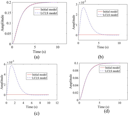
The comparisons of the right and left wheel velocity profiles due to the step of 0.2 m/s and the step of 0.1 m/s respectively of an initial model to those of the tuned LCLS model, are presented in Figure 3(a,b). The comparison of the resultant trajectories of the WMR is presented in Figure 3(c). Figure 4 shows the comparison of the step responses of the optimal LCLS model with those of the initial model. From the Figure 4 it can be seen that the desired time-domain specification has been embodied in the LCLS model with weighting matrices Q and R chosen optimally. The response of the off-diagonal elements of the LCLS model TFM is close to that of the corresponding elements of initial model TFM with a maximum error of the order of 10⁻³ m/s.

Figure 4. (a)–(d) Comparison of step responses of optimal LCLS model TFM to that of initial model TFM.

The present work evaluates the objective function in Equation (7) during a time interval T₂, which is the time taken by the WMR to complete two revolutions along the desired circular trajectory. The parameter τ can be calculated as τ = T₂/(Δt). In the present work, Δt is taken as 10⁻² s. The time taken for two revolutions of the WMR along the desired trajectory is calculated as 29.531 s [36].

The tuning of the weighting matrices presented in [25,26] is performed with the objective of mapping the desired time-domain specifications as a certain combination of weights of states and inputs. In the present work, the tuning of the weighting matrices considers the mapping of the interaction present in the initial model onto the LCLS model, in addition to the desired time-domain specifications.

6.1.2. Determination of OFCLS TFM

The present work illustrates the proposed algorithm for different G_c(s) structures as given in Table 1. The design of a practical PID using the proposed method is carried out by incorporating a low-pass filter along with the differentiator [37–39].

Table 1. The minimum value of the objective function obtained in the optimization procedure for the chosen controller structure.

	Degrees of numerator and denominator polynomials of elements of OFCLS TFM
Chosen controller structure	m^(1,1)	m^(1,2)	m^(2,1)	m^(2,2)	n	J2min
PI	8	8	8	8	10	1.0483e−06
Classical PID	9	9	9	9	10	2.3065e−06
PID having low-pass filter	10	10	10	10	12	6.5690e−07
PID^2 having low-pass filter	12	12	12	12	14	6.1883e−11
Lag	8	8	8	8	10	6.0703e−11
Type-I	7	7	7	7	10	5.9688e−11
Type-II	9	9	9	9	12	5.9691e−11
Type-III	11	11	11	11	14	5.9832e−11

The LCLS model is approximated to a TFM having the degrees of the numerator and the denominator polynomials as decided by the chosen controller structure, as shown in Table 1. In the present work, the desired frequency band of approximation and the value of M are taken as (10⁻³−10²) rad/s and 700 respectively. Optimal frequency points obtained in the case of each chosen controller structure are given in Appendix C. Equation (32(32) $\begin{array}{rl}\text{i}\text{.e}\text{.,}{G}_{CL}(s)& =G_P(s)G_c(s)[I-G_{CL}(s)]\end{array}$(32) ) is utilized in the EMM technique to obtain the unknown controller parameters (see Appendix D).

6.1.3. Comparison of frequency responses

The performance index J₂ in the first stage was minimized with the objective of matching the frequency response of the OFCLS to that of the LCLS model. The set of figures given in the first column of Figure 5 shows the comparison of the frequency response of the OFCLS with that of the desired LCLS model for PID-based controller structures, whereas the set of figures in the second column shows the comparison with lag-based controller structures.

Figure 5. (a)–(h) Comparison of the frequency response of LCLS to that of OFCLS.

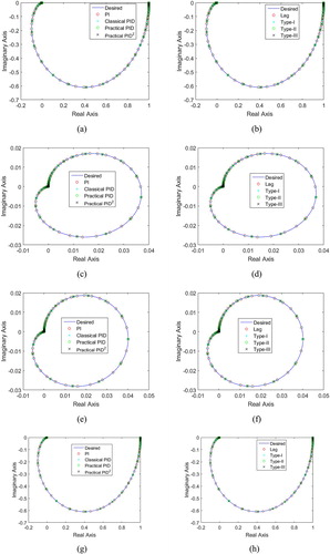
From Figure 5, it can be concluded that the frequency responses of G_d(s) and G_CL(s) match well.

6.1.4. Trajectory tracking

Figure 6(a,b) show the comparison of the trajectory of the WMR obtained by OFCLS TFM with that obtained with the desired LCLS model TFM, for PID-based G_c(s) structures and lag-based G_c(s) structures respectively.

Figure 6. (a), (b) Comparison of desired and actual trajectories. (c), (d) Desired and actual temporal variations in X-position. (e), (f) Desired and actual temporal variations in Y-position.

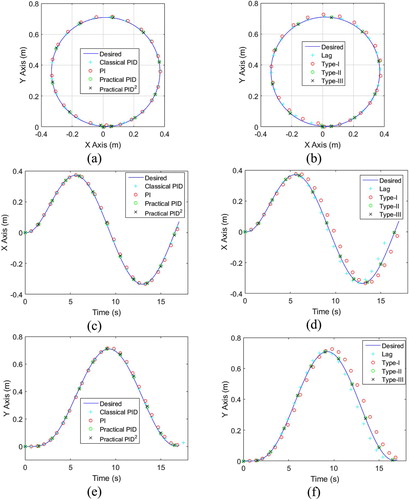
Figure 6(c,d) show the variation of the x-coordinates of the WMR for PID and lag-based G_c(s) structures respectively. Figure 6(e,f) show the variation of the y-coordinates of the WMR for PID and lag-based G_c(s) structures respectively. Figure 6 shows that the actual trajectory of the WMR using the designed controllers satisfactorily matches the desired trajectory. The computational time taken for each stage of the algorithm is shown in Table 2. The computational times shown are for MATLAB R2015b software running on a 3.3 GHz Intel(R) Core(TM) i5-4590 processor with 8 GB RAM.

Table 2. Computational time of the proposed algorithm.

Stage	Computational time (s)
I	270.573443
II	0.140385

6.2. Example 2

The proposed method has been utilized to design a decentralized G_c(s) for a 10th order MIMO plant taken from the literature [2]. The G_d(s) in the first stage of the algorithm for this example has been selected based on pole-zero excess as described in [2]. With this G_d(s), the algorithm is started using the AMM presented in Section 4. The step response of the G_d(s) is compared with that of G_CL(s), obtained using the proposed method and the method presented in the literature [2], as shown in Figure 7. Comparisons of the minimum value of the objective function (Equation (29)) and maximum absolute deviation obtained using the method presented in the literature [2] with the values obtained using the proposed method, are presented in Table 3. Table 3 shows that the proposed method of controller design is better in comparison to the method reported in [2] on integral squared error index. The G_c(s) parameters obtained using the proposed method are presented in Appendix 5.

Figure 7. (a)–(d). Comparison of step responses of the user-defined reference model to that of the OFCLS.

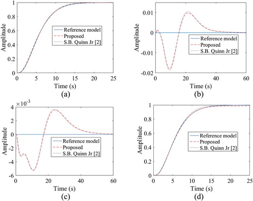
Figure 8. (a), (b) Desired and actual circular trajectories. (c), (d) Desired and actual temporal variations in X position. (e), (f) Desired and actual temporal variations in Y position.

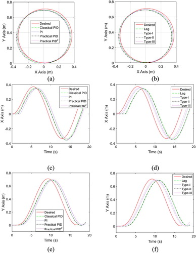
Table 3. The deviations in response of OFCLS ($\underset{ad}{\overset{(i,k)}{max}}$: the maximum absolute deviation in unit step response of (i, k)th element of OFCLS).

Method	J2	$\underset{ad}{\overset{(1,1)}{max}}$	$\underset{ad}{\overset{(1,2)}{max}}$	$\underset{ad}{\overset{(2,1)}{max}}$	$\underset{ad}{\overset{(2,2)}{max}}$
S.B. Quinn Jr [2]	0.2055	0.0114	0.0187	0.0052	0.0188
Proposed method	0.1556	0.0144	0.0180	0.0053	0.0114

7. Experimental results: Example 1

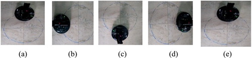
The operation of the WMR is based on the communication between the host computer and the target, QBot 2 [40]. The G_c(s) having the chosen structure and designed using the proposed algorithm is implemented on the host computer using the MATLAB-based Simulink software. The real-time control software, QUARC downloads real-time code generated from the host computer to the embedded computer mounted on the QBot 2 platform [40]. Figure 8(a,b) show the comparisons of the trajectory of the WMR obtained by OFCLS TFM with that obtained using the desired LCLS model TFM for PID-based G_c(s) structures and lag-based G_c(s) structures respectively, obtained in an experimental set-up. Figure 8(c,d) show the variation of x-coordinates of WMR for PID-based G_c(s) structures and lag-based G_c(s) structures respectively, obtained in an experimental set-up. Figure 8(e,f) show the variation of the y-coordinates of WMR for PID-based G_c(s) structures and lag-based G_c(s) structures respectively. Snapshots of the experimental output are presented in Figure 9(a–e). The blue circular trajectory is the desired trajectory, and the centre of the axle of the WMR tracks this trajectory. The deviations present in the experimental results are greater than those of the simulation results; this may be due to modelling errors incorporated during formulation of the mathematical representation of the plant dynamics.

Figure 9. (a)–(e). Real-time performance of WMR during circular trajectory tracking.

8. Conclusion

In this paper, a novel methodology for the design of suboptimal model-matching controllers for MIMO systems based on the SMF concept is presented. The conventional formulation of the reference model depends on the experience and prior knowledge of the designer about the requirement and performance of the plant. The advantage of the proposed reference model selection is that it involves the dynamics of the plant. The design procedure during the selection of the reference model encounters two problems. Firstly, interactions to be present in the designed closed-loop system are difficult to quantify as a specification. Secondly, in the LQRI design procedure, it is difficult to associate the desired time- or frequency-domain specifications with the elements of weighting matrices Q and R. The proposed reference model selection procedure addresses these two problems by formulating the problem as an optimization problem. The developed controller design algorithm is also compatible with user-defined reference models as illustrated in the second example.

As a part of the procedure in the first stage, a higher-order approximation method for MIMO lower-order systems based on the SMF concept is proposed. The LCLS model requires information regarding all the states for the purposes of implementation. The performance of the designed higher-order OFCLS mimics that of the lower-order LCLS model. Thus, the designed OFCLS can be termed suboptimal. The OFCLS is designed to have same denominator polynomial in all the elements of its TFM which results in its minimum realization. The developed algorithm also incorporates the complex poles and/or zeros in the SMF of an approximant. The SMF-based approximation ensures the steady-state matching of the reference model and OFCLS. The approximation procedure also ensures the stability of the OFCLS. Analysis of the closed-loop system can be performed at the end of the first stage itself.

In the second stage, the controller parameters are obtained using the EMM method with the information of the OFCLS and plant TFMs. In the EMM method, some of the unknown controller parameters can be assumed, taking into consideration the availability of hardware components during implementation. The rest of the controller parameters can be obtained by the solution of the resulting simultaneous equations. In this work, the filter coefficient present in the practical PID is kept constant at a value of 100, and the rest of the parameters are obtained as described. The proposed method for the controller design is illustrated by taking two examples from the literature. Work has also been carried out on utilizing the proposed algorithm for the design of fractional-order controllers for MIMO systems. This work will be reported elsewhere.

Disclosure statement

No potential conflict of interest was reported by the author(s).

Appendices

Appendix A. Determination of the Degree of the Numerator and Denominator Polynomials of the Elements of OFCLS TFM

Let $De{g}_n^{(i,k)}[\cdot ]$ stand for “degree of the numerator polynomial of (i,k)th element of the TFM” and $De{g}_d^{(i,k)}[\cdot ]$ stand for “degree of the denominator polynomial of (i,k)th element of the TFM”.

Let $De{g}_n^{(i,k)}[G_P(s)]=m_P^{(i,k)}$, $De{g}_d^{(i,k)}[G_P(s)]=n_P$, $De{g}_n^{(i,k)}[G_c(s)]=m_c^{(i,k)}$, $De{g}_d^{(i,k)}[G_c(s)]=n_c$, $De{g}_n^{(i,k)}[G_{CL}(s)]=m_{CL}^{(i,k)}$ and $De{g}_d^{(i,k)}[G_{CL}(s)]=n_{CL}$. Then, $De{g}_n^{(1,1)}[G_P(s)G_c(s)]=m_{Pc}^{(1,1)}=max(m_P^{(1,1)}+m_c^{(1,1)},m_P^{(1,2)}+m_c^{(2,1)})$, $De{g}_n^{(1,2)}[G_P(s)G_c(s)]=m_{Pc}^{(1,2)}=max(m_P^{(1,1)}+m_c^{(1,2)},m_P^{(1,2)}+m_c^{(2,2)})$, $De{g}_n^{(2,1)}[G_P(s)G_c(s)]=m_{Pc}^{(2,1)}=max(m_P^{(2,1)}+m_c^{(1,1)},m_P^{(2,2)}+m_c^{(2,1)})$, $De{g}_n^{(2,2)}[G_P(s)G_c(s)]=m_{Pc}^{(2,2)}=max(m_P^{(2,1)}+m_c^{(1,2)},m_P^{(2,2)}+m_c^{(2,2)})$, and $De{g}_d^{(i,k)}[G_P(s)G_c(s)]=n_{Pc}=n_P+n_c$.

The degrees of the numerator and denominator polynomials of the elements of OFCLS TFM are formulated as

$De{g}_n^{(1,1)}[G_{CL}(s)]=m_{CL}^{(1,1)}=max(n_{Pc}+m_{Pc}^{(1,1)},m_{Pc}^{(1,2)}+m_{Pc}^{(2,1)})$, $De{g}_n^{(1,2)}[G_{CL}(s)]=m_{CL}^{(1,2)}=max(n_{Pc}+m_{Pc}^{(1,2)},m_{Pc}^{(1,2)}+m_{Pc}^{(2,2)})$,

$De{g}_n^{(2,1)}[G_{CL}(s)]=m_{CL}^{(2,1)}=max(m_{Pc}^{(1,1)}+m_{Pc}^{(2,1)},n_{Pc}+m_{Pc}^{(2,1)})$, $De{g}_n^{(2,2)}[G_{CL}(s)]=m_{CL}^{(2,2)}=max(m_{Pc}^{(1,2)}+m_{Pc}^{(2,1)},n_{Pc}+m_{Pc}^{(2,2)})$, and $De{g}_d^{(i,k)}[G_{CL}(s)]=n_{CL}=max(2n_{Pc},m_{Pc}^{(1,2)}+m_{Pc}^{(2,1)})$.

Appendix B. Direction for Obtaining LCLS Model: Example 1

AB.1. Settings of GA

The weighting matrices $Q\in {\mathbb{R}}^{(n+p)\times (n+p)}$ and $R\in {\mathbb{R}}^{q\times q}$ of LQRI were taken as the diagonal matrices. The dynamic model of the plant [34] had n ( = 4) states and together with the p ( = 2) additional states of LQRI, the total states present in the LQRI becomes n + p ( = 6). Hence the number of parameters to be optimized for the weighting matrices Q and R were obtained as 8. Together with the pole location of off-diagonal elements of the initial model, the total number of parameters to be optimized nvars becomes nine. The set of optimal parameters ${\nu }_{op}^{(1)}$ has been chosen by utilizing MATLAB function “ga”. The optimal parameters obtained in this paper were obtained by selecting the lower and upper bound for the weighting matrices Q and R as zero and infinity respectively. The lower and upper bounds for the degree of interaction λ were set as 100 and 4500 respectively.

AB.2. Determination of the initial model and the LCLS model from ${\nu }_{op}^{(1)}$

The optimized values of the initial model and the LCLS model parameters obtained by using GA are λ = 3167.6, Q = diag(0.1454, 0.0086, 36.6894, 36.7116, 57.8158, 59.0674) and R = diag(0.0285, 114.1767).

The optimal gain matrix $K_{op}=\left[\begin{array}{cccccc}\text{2}\text{.8358}& \text{ - 0}\text{.1306}& \text{35}\text{.7622}& \text{0}\text{.0004}& \text{ - 45}\text{.0098}& \text{0}\text{.4337}\\ \text{ - 0}\text{.0012}& \text{0}\text{.0109}& \text{8}\text{.8187e - 08}& \text{0}\text{.4798}& \text{ - 0}\text{.0068}& \text{ - 0}\text{.7192}\end{array}\right]$

The parameters of the initial model are obtained as shown below:

$Coe[n_m^{(1,1)}(s)]$ = [−0.5, 0.1359, 4653], $Coe[d_m^{(1,1)}(s)]$= [1, 3170, 8448, 4654], $Coe[n_m^{(1,2)}(s)]$= $Coe[n_m^{(2,1)}(s)]$= [1], $Coe[d_m^{(1,2)}(s)]$= $Coe[d_m^{(2,1)}(s)]$ = [1, 3167.6], $Coe[n_m^{(2,2)}(s)]$= [−2, −3.864, 4651], $Coe[d_m^{(2,2)}(s)]$= [1, 3170, 8448, 4654],

where the numerator and denominator polynomials of $G_m^{(i,k)}(s)$ are denoted by $n_m^{(i,k)}(s)$ and $d_m^{(i,k)}(s)$ respectively.

The parameters of the LCLS model are obtained as shown below:

$Coe[n_d^{(1,1)}(s)]$ = [6.297e05, 3.912e09, 1.116e10, 6.119e09], $Coe[n_d^{(1,2)}(s)]$ = [−4205, 6.822e08, 3.998e08, −7.103e-07], $Coe[n_d^{(2,1)}(s)]$ = [1.166e05, 7.591e08, 3.914e08,0], $Coe[n_d^{(2,2)}(s)]$ = [8939, 3.884e09, 1.115e10, 6.119e09], $Coe[D_d(s)]$ = [1, 3.929e05, 2.4e09, 1.412e10, 2.81e10, 2.231e10, 6.119e09], where the numerator and denominator polynomials of $G_d^{(i,k)}(s)$ are denoted by $n_d^{(i,k)}(s)$ and $D_d(s)$ respectively.

Appendix C. Direction for Obtaining OFCLS: Example 1

The lower and upper bounds for the frequency points were determined as presented in [31]. The optimal frequency points ${\nu }_{op}^{(2)}$ obtained during the approximation procedure for different chosen controller structures are presented in Table A1.

Table A1. Optimal frequency points obtained during the first stage of the proposed algorithm.

Chosen controller	Optimal frequency points
PI	[ 0.3125,0.3250,0.4, 1.1625,1.1326,1.9249,1.2003,1.4,1.6001,1.9250,2.0007]
Classical PID	[0.0021,0.1704,0.4105,0.3593,0.8459,0.8764,0.9941,1.2726,1.684,2.0588,1.2392,1.2943]
Practical PID	[0.0003,0.1746,0.5515,0.5844,0.6666,0.8343,1,1.1666,1.3355,2,1.6666,1.8335,2]
Practical PID^2	[0.0030,0.1386,0.3337,0.4606,0.5483,0.8707,0.9557,1.2909,1.1451,1.6234,1.9909,1.5935, 197.2722,358.4262,555.6729,779.2029]
Lag	[0.4676,0.7512,75.7339,206.4056,311.3577,143.6814,226.6049,7.71469,625.1723,876.6793,988.1373]
Type-I	[0.1971,1.6911,0.5079,129.5588,158.1566,219.9116,202.0150,181.5280,222.3132,197.1013]
Type-II	[0.0024,0.9436,0.9594,103.0708,124.9799,237.5691,124.8871,79.6406,203.7030,394.4710,311.3046, 118.3724]
Type-III	[0.0043,0.1284,0.4591,0.6258,0.6707,1.080,1.5780,1.9264,1.8489,66.7960,43.2133,259.9185, 275.5172,548.7076,229.9250]

The determination of ${\nu }_{op}^{(2)}$ is followed by finding the solution of Equation (25), to obtain the coefficients of the SMF of OFCLS TFM. Now the stability preserving root selection strategy as mentioned in subsection 5.3 can be utilized to obtain the OFCLS TFM.

Appendix D. EMM technique for controller design

For a 2 × 2 MIMO system, the Equation (32) is represented as a function of the corresponding numerator and denominator polynomials as (A1) $\begin{array}{rl}& [\begin{array}{cc}{n}_P^{(1,1)}{d}_{CL}-n_P^{(1,1)}{n}_{CL}^{(1,1)}& -n_P^{(1,1)}{n}_{CL}^{(2,1)}\\ -n_P^{(1,1)}{n}_{CL}^{(1,2)}& n_P^{(1,1)}{d}_{CL}-n_P^{(1,1)}{n}_{CL}^{(2,2)}\\ n_P^{(2,1)}{d}_{CL}-n_P^{(2,1)}{n}_{CL}^{(1,1)}& -n_P^{(2,1)}{n}_{CL}^{(2,1)}\\ -n_P^{(2,1)}{n}_{CL}^{(1,2)}& n_P^{(2,1)}{d}_{CL}-n_P^{(2,1)}{n}_{CL}^{(2,2)}\end{array}\\ & \begin{array}{cc}{n}_P^{(1,2)}{d}_{CL}-n_P^{(1,2)}{n}_{CL}^{(1,1)}& -n_P^{(1,2)}{n}_{CL}^{(2,1)}\\ -n_P^{(1,2)}{n}_{CL}^{(1,2)}& n_P^{(1,2)}{d}_{CL}-n_P^{(1,2)}{n}_{CL}^{(2,2)}\\ n_P^{(2,2)}{d}_{CL}-n_P^{(2,2)}{n}_{CL}^{(1,1)}& -n_P^{(2,2)}{n}_{CL}^{(2,1)}\\ -n_P^{(2,2)}{n}_{CL}^{(1,2)}& n_P^{(2,2)}{d}_{CL}-n_P^{(2,2)}{n}_{CL}^{(2,2)}\end{array}]\left[\begin{array}{c}{n}_c^{(1,1)}\\ n_c^{(1,2)}\\ n_c^{(2,1)}\\ n_c^{(2,2)}\end{array}\right]\\ & =d_P{d}_c\left[\begin{array}{c}{n}_{CL}^{(1,1)}\\ n_{CL}^{(1,2)}\\ n_{CL}^{(2,1)}\\ n_{CL}^{(2,2)}\end{array}\right]\end{array}$(A1) The degrees of numerators and denominators on both sides of Equation (D.1) will be same. After cross multiplying, the coefficients of like terms are equated to form the non-homogeneous equation, the solution of which yields the unknown G_c(s) parameters.

Appendix E. Controller parameters obtained using the proposed method

AE.1. Example 1

The numerators and denominator of the obtained controller TFM for different chosen structures are as follows:

• PI

$n_c^{(1,1)}(s)=-\text{0}\text{.08569s}+\text{0}\text{.5224}$, $n_c^{(1,2)}(s)=\text{0}\text{.00197s}+\text{0}\text{.0244}$, $n_c^{(2,1)}(s)=\text{0}\text{.003418s}+\text{0}\text{.02505}$, $n_c^{(2,2)}(s)=-\text{0}\text{.08593s}+\text{0}\text{.5215}$, and ${\text{d}}_{\text{c}}\text{(s)}\text{ = }s$.

• Classical PID

$n_c^{(1,1)}(s)=\text{0}\text{.02357}{\text{s}}^{\text{2}}-\text{0}\text{.1256s}+\text{0}\text{.5425}$, $n_c^{(1,2)}(s)=-\text{0}\text{.003118}{\text{s}}^{\text{2}}+\text{0}\text{.007242s}+\text{0}\text{.02176}$, $n_c^{(2,1)}(s)=-\text{0}\text{.003898}{\text{s}}^{\text{2}}+\text{0}\text{.01002s}+\text{0}\text{.02175}$, $n_c^{(2,2)}(s)=\text{0}\text{.02376}{\text{s}}^{\text{2}}-\text{0}\text{.1263s}+\text{0}\text{.5417}$, and ${\text{d}}_{\text{c}}\text{(s)}\text{ = }s$.

• PID having low-pass filter

$n_c^{(1,1)}(s)=\text{2}\text{.237}{\text{s}}^{\text{2}}-\text{12}\text{.03s}+\text{54}\text{.26}$, $n_c^{(1,2)}(s)=-\text{0}.3014{\text{s}}^{\text{2}}+\text{0}\text{.7437s}+\text{2}\text{.171}$, $n_c^{(2,1)}(s)=-\text{0}\text{.3762}{\text{s}}^{\text{2}}+\text{1}\text{.021s}+\text{2}\text{.169}$, $n_c^{(2,2)}(s)=\text{2}\text{.255}{\text{s}}^{\text{2}}-\text{12}\text{.09s}+\text{54}\text{.19}$, and ${\text{d}}_{\text{c}}\text{(s)}\text{ = }{\text{s}}^{\text{2}}+100s$.

• PID² having low-pass filter

$n_c^{(1,1)}(s)=\text{0}\text{.8037}{\text{s}}^{\text{3}}+\text{0}\text{.5335}{\text{s}}^{\text{2}}-\text{10}\text{.22s}+\text{53}\text{.35}$, $n_c^{(1,2)}(s)=-\text{0}\text{.1117}{\text{s}}^{\text{3}}+\text{0}\text{.023}{\text{s}}^{\text{2}}+\text{0}\text{.4043s}+\text{2}\text{.3}$, $n_c^{(2,1)}(s)=-\text{0}\text{.1389}{\text{s}}^{\text{3}}+\text{0}\text{.02329}{\text{s}}^{\text{2}}+\text{0}\text{.6031s}+\text{2}\text{.329}$, $n_c^{(2,2)}(s)=\text{0}\text{.8105}{\text{s}}^{\text{3}}+\text{0}\text{.5326}{\text{s}}^{\text{2}}-\text{10}\text{.26s}+\text{53}\text{.26}$, and ${\text{d}}_{\text{c}}\text{(s)}\text{ = }{\text{s}}^{\text{3}}+100s$.

• Lag

$n_c^{(1,1)}(s)=-0.08609s+0.5088$, $n_c^{(1,2)}(s)=\text{0}\text{.00394s}+\text{0}\text{.02289}$, $n_c^{(2,1)}(s)=\text{0}\text{.005704s}+\text{0}\text{.0234}$, $n_c^{(2,2)}(s)=-\text{0}\text{.08648s}+\text{0}\text{.508}$, and ${\text{d}}_{\text{c}}\text{(s)}\text{ = }\text{s - 0}\text{.03173}$.

• Type-I

$n_c^{(1,1)}(s)=\text{0}\text{.4537}$, $n_c^{(1,2)}(s)=\text{0}\text{.0263}$, $n_c^{(2,1)}(s)=\text{0}\text{.02822}$, $n_c^{(2,2)}(s)=\text{0}\text{.4525}$, and ${\text{d}}_{\text{c}}\text{(s)}\text{ = }\text{s}$.

• Type-II

$n_c^{(1,1)}(s)=\text{0}\text{.1374s}+\text{1}\text{.515}$, $n_c^{(1,2)}(s)=\text{0}\text{.03844s}+\text{0}\text{.06288}$, $n_c^{(2,1)}(s)=\text{0}\text{.0464s}+\text{0}\text{.06298}$, $n_c^{(2,2)}(s)=\text{0}\text{.135s}+\text{1}\text{.513}$, and ${\text{d}}_{\text{c}}\text{(s)}\text{ = }{\text{s}}^{\text{2}}+\text{2}\text{.751s}$.

• Type-III

$n_c^{(1,1)}(s)=\text{0}\text{.1204}{\text{s}}^{\text{2}}+\text{1}\text{.98s}+\text{4}\text{.649}$, $n_c^{(1,2)}(s)=-\text{0}\text{.001187}{\text{s}}^{\text{2}}+\text{0}\text{.2315s}+\text{0}\text{.1666}$, $n_c^{(2,1)}(s)=\text{0}\text{.001138}{\text{s}}^{\text{2}}+\text{0}\text{.2632s}+\text{0}\text{.163}$, $n_c^{(2,2)}(s)=\text{0}\text{.1197}{\text{s}}^{\text{2}}+\text{1}\text{.968s}+\text{4}\text{.643}$, and ${\text{d}}_{\text{c}}\text{(s)}\text{ = }{\text{s}}^{\text{3}}+\text{5}\text{.878}{\text{s}}^{\text{2}}+\text{8}\text{.456s}$.

AE.2. Example 2

$n_c^{(1,1)}(s)=\text{0}\text{.0002189}{\text{s}}^{\text{2}}+\text{3}\text{.184}\text{s}+\text{0}\text{.8242}$, ${\text{d}}_c^{(1,1)}\text{(s)}=\text{0}\text{.2003}{\text{s}}^{\text{2}}+\text{4}\text{.902s}$, $n_c^{(2,2)}(s)=\text{0}\text{.06077}{\text{s}}^{\text{2}}+\text{1}\text{.791s}+\text{0}\text{.4536}$, and ${\text{d}}_c^{(2,2)}\text{(s)}\text{ = }\text{0}\text{.3664}{\text{s}}^{\text{2}}+\text{2}\text{.802s}$.

References

- Szita G, Sanathanan CK. A model matching approach for designing decentralized MIMO controllers. J Franklin Inst. 2000;337(6):641–660.
- Quinn SB, Sanathanan CK. Model matching control for multivariable systems—I. Stable plants. J Franklin Inst. 1990;327(5):699–712.
- Quinn SB, Sanathanan CK. Model matching control for multivariable systems—II. Unstable plants. J Franklin Inst. 1990;327(5):713–729.
- Szita G, Sanathanan CK. Model matching controller design for disturbance rejection. J Franklin Inst. 1996;333(5):747–772.
- Paraskevopoulos PN. Exact model-matching of 2-D systems via state feedback. J Franklin Inst. 1979;308(5): 475–486.
- Das SK, Pota HR, Petersen IR. Multivariable negative-imaginary controller design for damping and cross coupling reduction of nanopositioners: a reference model matching approach. IEEE/ASME Trans Mechatron. 2015;20(6):3123–3134.
- Beevi PF, Kumar TS, Jacob J, et al. Novel two degree of freedom model matching controller for set-point tracking in MIMO systems. Comput Electr Eng. 2017;61:1–14.
- Damodaran S, Kumar TK, Sudheer AP. Model-matching fractional-order controller design using AGTM/AGMP matching technique for SISO/MIMO linear systems. IEEE Access. 2019;7:41715–41728.
- Beevi PF, Kumar TS, Jacob J. Novel two degree of freedom model matching controller for desired tracking and disturbance rejection. Stud Inf Control. 2017;26(1):105–114.
- Luan X, Chen Q, Liu F. Centralized PI control for high dimensional multivariable systems based on equivalent transfer function. ISA Trans. 2014;53(5):1554–1561.
- Sanathanan CK, Quinn SB. Controller design via the synthesis equation. J Franklin Inst. 1987;324(3):431–451.
- Prajapati AK, Prasad R. Model order reduction by using the balanced truncation and factor division methods. IETE J Res. 2019 Nov 2;65(6):827–842.
- Prajapati AK, Prasad R. A new model order reduction method for the design of compensator by using moment matching algorithm. Trans Inst Meas Control. 2020 Feb;42(3):472–484.
- Lin JM, Han KW. Model reduction for control systems with parameter variations. J Franklin Inst. 1984;317(2): 117–133.
- Paraskevopoulos PN, King RE. Multivariable process-controller design by approximate model-matching. IEEE Trans Ind Electron Contr Instrum. 1978;IECI-25:50–54.
- Tzafestas S, Paraskevopoulos P. On the exact model matching controller design. IEEE Trans Autom Control. 1976;21(2):242–246.
- Paraskevopoulos PN. Exact model matching of linear time-varying systems. Proc Inst Electr Eng. 1978;125(1): 66–70.
- Paraskevopoulos PN, Koumboulis FN, Anastasakis DF. Exact model matching of generalized state space systems. J Optim Theor Appl. 1993;76(1):57–85.
- Kimura G, Matsumoto T, Takahashi S. A direct method for exact model matching. Syst Control Lett. 1982;2(1):53–56.
- Ye J. Adaptive control of nonlinear PID-based analog neural networks for a nonholonomic mobile robot. Neurocomputing. 2008;71(7):1561–1565.
- Normey-Rico JE, Alcalá I, Gómez-Ortega J, et al. Mobile robot path tracking using a robust PID controller. Control Eng Pract. 2001;9(11):1209–1214.
- Hu Q, Xu L, Zhang A. Adaptive backstepping trajectory tracking control of robot manipulator. J Franklin Inst. 2012;349(3):1087–1105.
- Peng J, Yu J, Wang J. Robust adaptive tracking control for nonholonomic mobile manipulator with uncertainties. ISA Trans. 2014;53(4):1035–1043.
- Lin F, Lin Z, Qiu X. LQR controller for car-like robot. 35th Chinese Control Conference; Chengdu, China; 2016. p. 2515–2518.
- Liu C, Pan J, Chang Y. PID and LQR trajectory tracking control for an unmanned quadrotor helicopter: experimental studies. 35th Chinese Control Conference; 2016. p. 10845–10850.
- Pourshaghaghi HR, Jaheh-Motlagh MR, Jalali AA. Optimal feedback control design using genetic algorithm applied to inverted pendulum). Industrial Electronics; 2007. p. 263–268.
- Hassani K, Lee WS. Optimal tuning of linear quadratic regulators using quantum particle swarm optimization). Proceedings of the International Conference Control, Dynamic Robotics; 2014. p. 14–15.
- Stefanescu RM, Prioroc CL, Stoica AM. Weighting matrices determination using pole placement for tracking maneuvers. UPB Sci Bull, Series D. 2013;75(2):31–41.
- Chen CP, Tsay YT. A squared magnitude continued fraction expansion for stable reduced models. Int J Syst Sci. 1976;7(6):625–634.
- Mahata S, Banerjee S, Kar R, et al. Revisiting the use of squared magnitude function for the optimal approximation of (1+ α)-order Butterworth filter. AEU-Int J Electron Commun. 2019;110(152826). p. 1–11.
- Khanra M, Pal J, Biswas K. Use of squared magnitude function in approximation and hardware implementation of SISO fractional order system. J Franklin Inst. 2013;350(7):1753–1767.
- Hwang C, Chen MY. Stable linear system reduction via a multipoint squared-magnitude continued-fraction expansion. IEE Proc D-Control Theor Appl. 1988;135(6):441–444.
- Chen TC, Chang CY, Han KW. Model reduction using the stability-equation method and the Padè approximation method. J Franklin Inst. 1980;309(6):473–490.
- Damodaran S, Kumar TK, Sudheer AP. Design and implementation of GA tuned PID controller for desired interaction and trajectory tracking of wheeled mobile robot. Proceedings of the Advances in Robotics, ACM. 2017. p. 34.
- Tymerski R, Rytkonen F. Control System Design. 2012.
- Haddadi A, Martin P, Fulford C. Quanser QBot 2 Complete Workbook (Instructor). Quanser, Canada; 2015.
- Li Y, Ang KH, Chong GC. PID control system analysis and design. IEEE Control Syst. 2006;26(1):32–41.
- Liu J, Lam J, Shen M, et al. Non-fragile multivariable PID controller design via system augmentation. Int J Syst Sci. 2017;48(10):2168–2181.
- Huba M, Vrancic D, Bistak P. PID control with higher order derivative degrees for IPDT plant models. IEEE Access. 2021;9:2478–2495.
- User manual. QBot 2 for QUARC set up and configuration. Quanser, Canada; 2015.