H∞ optimal control of vehicle active suspension systems in two time scales

Abstract

In this paper, a novel H_∞ control method in two time scales is proposed for active suspension systems. Two time scales are considered based on the natural time scale separation existing in the active suspension systems, i.e. the sprung mass part corresponding to the fast dynamics and the unsprung mass part corresponding to the slow dynamics. Singular perturbation theory is used to establish a dual time scale active suspension model and design a H_∞ controller. Compared with the commonly used H_∞ controller, the time-sharing dynamic characteristics make the proposed two time scales H_∞ controller have better dynamic response when encountering dynamic road input, so as to better meet the control performance requirements of active suspension. The effectiveness of the proposed H_∞ control method in two time scales is illustrated through co-simulations.

KEYWORDS:

• H_∞ control
• two time scales
• active suspension
• optimal control

1. Introduction

In order to pursue the comfort and safety of vehicles, more and more researchers have focused on the design and control of active suspension in the past decades [1–3]. As we all know, suspension is the general term of all force transmission connecting devices between the vehicle frame (or load-bearing body) and the axle (or wheel). Its function is to transfer the force and torque between the wheel and the frame, buffer the impact force transmitted from uneven road surface to the frame or body, and reduce the vibration caused by it, so as to ensure the smooth running of the car. Specifically, active suspension systems, also known as active guidance suspension systems and dynamic variable suspension systems, can control the vibration and height of vehicle body by changing the height, shape and damping of suspension system. It can mainly improve the performance of vehicle operation stability and riding comfort. Therefore, active suspension represents the development direction of automobile suspension in the future and a large number of scholars have carried out a lot of research on the key control problems, e.g. LQG control [4], adaptive control [5], sliding mode control [6], robust control [7], backstepping control [8], etc. The control of active suspension systems, however, poses a major challenge due to the unknown road input, high order and strong coupling characteristics. On the other hand, from the perspective of practical application in vehicles, the potential poor transient response (e.g. overshoot, sluggish convergence) of the above control methods may result in performance degradation, hazards and even cause hardware damage.

Singular perturbation analysis of complex nonlinear systems provides a valuable tool that simplifies the burden of designing appropriate control laws and guaranteeing the asymptotic stability of the original nonlinear system. The singular perturbation theory (SPT) was first introduced by Friedrichs and Wasow in the 1940 [9]. In Russia, mainly at Moscow State University, research activity on singular perturbations for ordinary differential equations, originated and developed by Tikhonov in the 1950s [10]. An excellent survey of the historical development of singular perturbations is found in a book by O’Malley [11]. Other historical surveys concerning the research activity in singular perturbation theory at Moscow State University and elsewhere can are found [12,13]. The curse of dimensionality coupled with stiffness poses formidable computational complexities for the analysis and design of multiple time scale systems. This time-scale approach is asymptotic, that is, exact in the limit as the ratio ϵ of the speeds of the slow versus the fast dynamics tends to zero. When ϵ is small, approximations are obtained from reduced-order models in separate time scales [14], and this separation of time scales helps to reduce the order of complexity of the systems being controlled [15].

A car suspension system is a typical two-time-scale nonlinear dynamic system which has fast and slow dynamics. The ride quality and the road holding are relevant to the slow and fast motions respectively. A review of the literature of singular perturbation methods applied to suspension systems can be traced back to the early works of Li and Wang [16], to the work conducted by the authors Ando [17], Kim [18], Carbinatto [19], Aghazadeh [20] and Paarya [21], related to the theoretically addressing of stability issues for modelling and controller design using singular perturbations theory. The studies described above take account of the difference between the time response of suspension dynamics and obtain the suspension model which has two sub-systems. For such a model the singular perturbation method [22] is applied to design the suspension control system. For the slow and fast subsystems, control laws are designed to improve each property. The total control law is obtained as a composite of the two control laws for the two subsystems. This procedure makes the design of the control law very clear, because the two properties can be considered separately.

H_∞ control with strong robustness and good optimization performance has attracted much attention in the control filed [23–25], and is one of prospective control methodologies for active suspension systems [26,27]. Unfortunately, the nonlinear, high order and strong coupling characteristics of the active suspension systems make it very complex for the H_∞ controller design. In view of this situation, the core idea of this paper is to design the controller by combining SPT and H_∞ theory based on the reduced model, which could greatly simplify the analysis process and provides a good possibility to achieve the high-performance control objectives at the same time. Although the original suspension system is hard to design the H_∞ controller due to the complex dynamic characteristics, the singular perturbation method can be linearized easily into two reduced subsystems, which is the most significant advantage of the design method proposed in this paper.

This study proposes a novel H_∞ control method of active suspension systems considering the time scales. In summary, the main contributions of this paper are as follows. Firstly, the two-time scales suspension model considering the dynamic characteristics of different time scales caused by body resonance and wheel resonance is established. Secondly, this separation of time scales helps to reduce the order of complexity of the systems being controlled, which leads to a high performance H_∞ controller design, so that the transient response performance requirements in terms of ride comfort and suspension space limitation for active suspension systems is guaranteed. Finally, co-simulations between Carsim and Simulation verifies the improved performance of the proposed H_∞ control method in two time scales compared with the conventional H_∞ control method.

The paper is organized in six sequential sections. Quarter-car suspension system is given in Section 2. The general H_∞ controller is designed in Section 3. Two time scales H_∞ controller design is demonstrated in Section 4. Co-simulation results illustrating the effectiveness of the proposed scheme are presented and discussed in Section 5. Conclusions are summarized in Section 6.

2. Quarter-car suspension system

Generally speaking, when modelling a real complex vibration system, the more complex the model is, the closer it is to the actual situation, and the more realistic simulation can be carried out, but the analysis is often difficult. On the other hand, the simpler the model is, the easier the analysis is, but the error of the results obtained is too large. Therefore, when establishing the mechanical model of vibration system, there is always a tradeoff between simplified expression and realistic simulation. In the study of suspension ride comfort, the complex vehicle vibration system can be simplified. In this paper, the commonly used quarter suspension model which can accurately express the vehicle ride comfort performance is selected as the research object [28,29]. Half of the active suspension structure can be simplified as a dual mass vibration system, as shown in Figure 1.

Figure 1. Quarter-car active vehicle suspension systems.

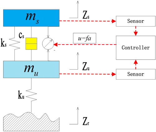
The mathematical model of active suspension systems shown in Figure 1 is given as (1) $\begin{array}{rl}{\ddot{z}}_s& =-\frac{k_s}{m_s}\left(z_s-z_u\right)-\frac{c_s}{m_s}\left({\dot{z}}_s-{\dot{z}}_u\right)+\frac{1}{m_s}{f}_a\\ {\ddot{\mathrm{z}}}_u& =\frac{k_s}{m_u}\left(z_s-z_u\right)+\frac{c_s}{m_u}\left({\dot{z}}_s-{\dot{z}}_u\right)\\ & -\frac{k_u}{m_u}\left(z_u-z_r\right)+\frac{1}{m_u}{f}_a\end{array}$(1) where a spring k_s, a damper c_s and an active force actuator f_a constitute the main three parts of suspension systems. When the actuator output force is zero, it is equivalent to the passive suspension systems. m_s is the sprung mass and m_u is the unsprung mass which represent the quarter equivalent mass of the vehicle body and the equivalent mass of the tire assembly system, respectively; Vertical stiffness coefficient of the tire is denoted by k_u; z_s, z_u and z_r are vertical displacements of the sprung mass, unsprung mass and road, respectively.

In order to derive the state space form of the quarter car active suspension systems with hydro-pneumatic suspension actuators, we define the state variables as $x_1=z_s-z_u,x_2={\dot{z}}_s,x_{\text{3}}=z_u-z_r,x_{\text{4}}={\dot{z}}_u$, where $z_s-z_u$ is the suspension deflection, ${\dot{z}}_s$ is the velocity of sprung mass, $z_u-z_r$ is the tire deflection, ${\dot{z}}_u$ is the velocity of unsprung mass. Then, Equation (1) can be further rewritten in the following state space form (2) $\dot{x}=Ax+B_{\text{1}}u+B_{\text{2}}{\dot{z}}_r$(2) where $\begin{array}{rl}A& =\left[\begin{array}{cccc}0& 1& 0& -1\\ -\frac{k_s}{m_s}& -\frac{c_s}{m_s}& 0& \frac{c_s}{m_s}\\ 0& 0& 0& 1\\ \frac{k_s}{m_u}& \frac{c_s}{m_u}& -\frac{k_u}{m_u}& -\frac{c_s}{m_u}\end{array}\right],\\ B_{\text{1}}& =\left[\begin{array}{c}0\\ \frac{1}{m_s}\\ 0\\ -\frac{1}{m_u}\end{array}\right],B_2=\left[\begin{array}{c}0\\ 0\\ -1\\ \frac{b_t}{m_u}\end{array}\right].\end{array}$

3. H∞ controller design

The objective of the controller design for the active suspension systems should consider the following three tasks [30]:

Firstly, the ride comfort of the car is mainly reflected by ride comfort, so the acceleration of the sprung mass should be controlled to the minimum as far as possible. When the vehicle is running on the road, it is necessary to ensure that the tire does not leave the ground, so the dynamic load between the tire and the ground should be less than the static load, i.e. (3) $k_u(z_u-z_r)<(m_s+m_u)g$(3) In addition, the dynamic travel of the suspension should be controlled within the maximum dynamic travel $S_{max}$, otherwise frequent impact of the limit block will reduce the riding comfort and handling of the vehicle, i.e. (4) $|z_s-z_u|\le S_{max}$(4)

Lastly, the generated force from the actuator which is used to drive the motion of suspension system should also be within the maximum limit, i.e. (5) $|f_a|\le F_{max}$(5) From the above three tasks as shown in (3), (4) and (5), the total performance output and constraint output can be defined as (6) ${\text{z}}_1={\ddot{z}}_s,z_2=\left[\begin{array}{c}\frac{\left(z_s-z_u\right)}{S_{max}}\\ \frac{k_u\left(z_u-z_r\right)}{\left(m_s+m_u\right)g}\\ \frac{f_a}{F_{max}}\end{array}\right]$(6)

Then the dynamics of (2) along (6) can be represented as (7) $\left\{\begin{array}{l}\dot{x}=Ax+B_{1}w+B_{2}u\\ z_1=C_{1}x+D_{1w}w+D_{1u}u\\ z_2=C_{2}x+D_{2w}w+D_{2u}u\end{array}\right.$(7) where $x$ is the state variable, $\omega$ is the road excitation, $u$ is the control input, $z_1$ is the performance output, $z_{\text{2}}$ is the constraint output, $C_1,D_{1w},D_{1u}u,C_2,D_{2w},D_{2u}$ are corresponding matrices.

For the $H_{\mathrm{\infty }}$ controller design, we define the state feedback gain matrix as K, then the feedback form for admissible optimal control u* can be derived as (8) $u^{\ast }=Kx$(8) Substituting (8) into (7), we have the following closed-loop system (9) $\left\{\begin{array}{l}\dot{x}=A_{c1}x+B_{1}w\\ z_1=C_{c1,1}x+D_{1w}w\\ z_2=C_{c1,2}x+D_{2w}w\end{array}\right.$(9) where $A_{c1}=A+B_{2u}K,C_{\text{c}1,1}=C_1+D_{1u}K,C_{\text{c}1,2}=C_2+D_{2u}K.$

For the active suspension closed-loop control system as described in (9), the design of $H_{\mathrm{\infty }}$ controller can be described as

1. The closed-loop system including the controlled target is stable;

2. The minimum $H_{\mathrm{\infty }}$ norm from disturbance $\omega$ to output z₁ is guaranteed;

3. z₂ should be suppressed in time domain to satisfy the output constraint as much as possible.

Theorem 3.1:

[31] Given a positive number $\alpha$, if there exist matrices $Q=Q^T>0$ and $Y$ such that the semi definite programming problem satisfies the following inequality (10) $\begin{array}{rl}& \left(\begin{array}{ccc}\begin{array}{c}AQ+Q{A}^T\\ +B_{\text{u}}Y+Y^T{B}_u\end{array}& B_w& {(C_{1}Q+D_{1u}Y)}^T\\ B_w^T& -{\gamma }^{2}I& D_{1w}^T\\ C_{1}Q+D_{1u}Y& D_{1w}& -I\end{array}\right)<0,Q>0\\ & \left(\begin{array}{cc}\frac{{\text{z}}_{\text{2i,max}}^{\text{2}}}{\alpha }& {\text{C}}_{\text{2,i}}Q+D_{2u,i}Y\\ {({\text{C}}_{\text{2,i}}Q+D_{2u,i}Y)}^T& Q\end{array}\right)>0\end{array}$(10) then there exists an optimal solution $\left({\gamma }_{\ast },Q_{\ast },Y_{\ast }\right).$ A state feedback solution of the $H_{\mathrm{\infty }}$ controller for active suspension can thus be expressed as $K=Y_{\ast }{Q}_{\ast }^{-1}$ and satisfy the following conditions

1. The closed-loop system is stable;

2. For all energy bounded interference inputs, the anti-interference level is ${\gamma }_{\ast }$;

3. If the energy level of the disturbance is less than $\frac{\alpha \text{ - x}{\left(0\right)}^T{Q}_{\ast }^{-1}x\left(0\right)}{{\gamma }_{\ast }^2}$, the constrained output satisfies the required constrained condition as shown in (6).

Remark 3.1:

Given a positive number $\alpha$, the above optimization problem (10) is convex and solvable with LMI. In order to solve the semidefinite programming problem by LMI tool, $\alpha$ needs to be set in advance. Since $x\left(0\right)\in$ ${\mathrm{\Omega }}_1(P,\alpha ,w_{max})$, it’s easy to get the relationship between $\alpha$ and $w_{max}$. i.e. $\alpha \ge {\gamma }^2{w}_{max}.$ By solving the above inequality (10) with LMI toolbox, the feedback control gain can be obtained.

4. Two time scales H_∞ controller design

4.1. Fast and slow decomposition of singularly perturbed systems

Consider the following singularly perturbed system [32] (11) $\begin{array}{rl}{\dot{x}}_1\left(t\right)& =A_{11}{x}_{\text{1}}\left(t\right)+A_{12}{x}_{\text{2}}\left(t\right)+B_{1}u\left(t\right)\end{array}$(11) (12) $\begin{array}{rl}ϵ{\dot{x}}_2\left(t\right)& =A_{21}{x}_{\text{1}}\left(t\right)+A_{22}{x}_{\text{2}}\left(t\right)+B_{2}u\left(t\right)\end{array}$(12) (13) $\begin{array}{rl}y\left(t\right)& =C_1{x}_{\text{1}}\left(t\right)+C_2{x}_{\text{2}}\left(t\right)\\ x_1\left(0\right)& =x_1^0,x_2\left(0\right)=x_2^0\end{array}$(13) where $x_1\left(t\right)\in R^n$ and $x_{\text{2}}\left(t\right)\in R^m$ are slow and fast state variables, respectively, $ϵ$ is the small positive parameter which indicates different time scales. $u\left(t\right)\in R^p$ is the control input vector, $y\left(t\right)\in R^q$ is system output.

Assumption 4.1:

[33] The basic assumption of singular perturbation theory is that the slow variable keeps normal in the process of fast variable, and when the change of slow variable is obvious, the transient process of fast variable has ended and reached its quasi steady state.

It is assumed that matrix $A_{\text{22}}$ is nonsingular and the variable $x_{\text{2}}\left(t\right)$ is asymptotically stable, when $ϵ\to \text{0}$, the system (11–13) degenerates into (14) $\begin{array}{rl}{\dot{x}}_{1s}& =A_{11}{x}_{1s}+A_{12}{x}_{\text{2}s}+B_1{u}_s\end{array}$(14) (15) $\begin{array}{rl}\text{0}& =A_{21}{x}_{\text{1}s}+A_{22}{x}_{\text{2}s}+B_2{u}_s\end{array}$(15) (16) $\begin{array}{rl}{y}_s& =C_1{x}_{\text{1s}}+C_2{x}_{\text{2s}}\end{array}$(16) $\begin{array}{rl}{x}_{1s}\left(0\right)& =x_1^0\end{array}$From (15), we have (17) $x_{\text{2}s}=-A_{22}^{-1}\left(A_{21}{x}_{\text{1}s}+B_2{u}_s\right)$(17) where $x_{\text{2}s}$ is the quasi steady state value of fast state.

Then, substituting (17) into (14) and (16), one obtains (18) $\begin{array}{rl}{\dot{x}}_{1s}& =A_{\text{0}}{x}_{1s}+B_{\text{0}}{u}_s\end{array}$(18) (19) $\begin{array}{rl}{y}_s& =C_{\text{0}}{x}_{1s}+D_{\text{0}}{u}_s\end{array}$(19) where $A_0=A_{11}-A_{12}{A}_{22}^{-1}{A}_{21}$, $B_0=B_1-A_{12}{A}_{22}^{-1}{B}_{21}$, $C_0=C_1-C_2{A}_{22}^{-1}{A}_{21}$, $D_0=-C_2{A}_{22}^{-1}{B}_2.$

One can get approximate solution of $x_{\text{1}s}$ by solving (18) and (19). In order to obtain the correction term, we assume that the slow variable $x_{\text{1}}$ remain unchanged in the time interval of the transient process. i.e. $x_1=x_{1s}=constant,$ ${\dot{x}}_{1s}=0.$ Then from (12) and (15), we have (20) $ϵ({\dot{x}}_{\text{2}}-{\dot{x}}_{\text{2s}})=A_{22}(x_{\text{2}}-x_{\text{2s}})+B_2(u-u_s)$(20) We define ${\dot{x}}_f={\dot{x}}_{\text{2}}-{\dot{x}}_{\text{2s}},u_f=u-u_s,y_f=y-y_s$, then from (20), the equations describing the fast changing states can be obtained as (21) $\begin{array}{rl}ϵ{\dot{x}}_f& =A_{22}{x}_f+B_2{u}_f\end{array}$(21) (22) $\begin{array}{rl}{x}_f\left(0\right)& =x_2^0-x_{2s}\left(0\right)\end{array}$(22) (23) $\begin{array}{rl}{y}_f& =C_2{x}_f\end{array}$(23) In order to solve x, we do scale transformation as (24) $\tau =\frac{t}{ϵ}$(24) Then (21) can be rewritten as (25) $\begin{array}{rl}\frac{d{x}_f}{d\tau }& =A_{22}{x}_f\left(\tau \right)+B_2{u}_f\end{array}$(25) (26) $\begin{array}{rl}{x}_f\left(0\right)& =x_2^0+A_{22}^{-1}{A}_{21}{x}_{\text{1}s}\left(0\right)\end{array}$(26) (27) $\begin{array}{rl}{y}_f& =C_2{x}_f\left(\tau \right)\end{array}$(27) Thus, $x_f\left(\tau \right)$ can be obtained by solving (25)–(27).

Definition 4.1:

[22] Let $x\left(ϵ\right)$ be a matrix function of positive scalar $ϵ$, when $ϵ\le {ϵ}^{\ast }$, if there are positive constant numbers $c$ and ${ϵ}^{\ast }$ satisfy the condition $||x\left(ϵ\right)||\le c{ϵ}^{\ast }$, then we call $x\left(ϵ\right)$ to be $o\left(ϵ\right)$.

The complete solution of the singularly perturbed system (11)–(13) is the sum of approximate solution and correction term. i.e. (28) $\begin{array}{rl}{x}_1& =x_{1s}\left(t\right)+o(ϵ{)}^{\ast }\end{array}$(28) (29) $\begin{array}{rl}{x}_{\text{2}}& =x_{\text{2}s}\left(t\right)+x_f\left(\tau \right)+o\left(ϵ\right)\\ & =-A_{22}^{-1}{A}_{21}{e}^{A_{0}t}{x}_1^0\\ & +e^{A_{22}t/ϵ}(x_2^0+A_{22}^{-1}{A}_{21}{x}_1^0)+o\left(ϵ\right)\end{array}$(29) It can be seen from (29) that if $x_{\text{2}}$ is asymptotically stable, the fast changing component $x_f$ of variable $x_{\text{2}}$ decays rapidly, and $x_f$ only has an important influence in the very short time when the transient process begins.

4.2. Two time scales H_∞ controller

In fact, through frequency domain analysis, the automobile suspension system is decomposed into a slow subsystem and a fast subsystem. These two subsystems are respectively related to road holding force and driving comfort. Hence, we can define the two time scales parameter as (30) $\begin{array}{rl}ϵ& =\frac{Naturalfrequenciesofvehiclebody}{naturalfrequenciesoftires}\\ & =\frac{\sqrt{k_s/m_s}}{\sqrt{k_u/m_u}}\end{array}$(30) Based on the singular perturbation theory, setting

$x_1=z_s-z_u,x_2={\dot{z}}_s$ as the slow variables, $x_{\text{3}}=z_u-z_r,x_{\text{4}}={\dot{z}}_u$ as the fast variables and u as the input, one can get the singularly perturbed suspension model, such that (31) $\begin{array}{l}\dot{x}=A\left(ϵ\right)x+B_1\left(ϵ\right)+B_2\left(ϵ\right)u\\ z=C_1\left(ϵ\right)x+D_{12}\left(ϵ\right)u\\ y=Ku\end{array}$(31) where $A\left(ϵ\right)=\left[\begin{array}{cc}{A}_{11}\left(ϵ\right)& A_{12}\left(ϵ\right)\\ \frac{A_{21}\left(ϵ\right)}{ϵ}& \frac{A_{22}\left(ϵ\right)}{ϵ}\end{array}\right]$, $B_1=\left[\begin{array}{c}{B}_{11}\left(ϵ\right)\\ \frac{B_{21}\left(ϵ\right)}{ϵ}\end{array}\right]$,$C_1\left(ϵ\right)=\left[\begin{array}{cc}{C}_{11}\left(ϵ\right)& C_{12}\left(ϵ\right)\end{array}\right]$.

According to the singularly perturbed boundary layer method as depicted in Section 4.1, the fast and slow decomposition of the suspension system (31) is obtained as (32) $\begin{array}{rl}& Fast:\begin{array}{l}{\dot{x}}_f=A_{22}{x}_f+B_{21}w+B_{22}u\\ z=C_1{x}_f+D_{12}u\\ u=K_{f}x\end{array}\end{array}$(32) (33) $\begin{array}{rl}& Slow:\begin{array}{l}{\dot{x}}_s=A_0{x}_f+B_{10}w+B_{20}u\\ z=C_{10}{x}_f+D_{10}u-C_{12}{A}_{22}^{-1}{B}_{21}w\\ u=K_{s}x\end{array}\end{array}$(33) where $A_0=A_{11}-A_{12}{A}_{22}^{-1}{A}_{21}$, $B_{10}=B_{11}-A_{12}{A}_{22}^{-1}{B}_{21}$, $C_{10}=C_{11}-C_{12}{A}_{22}^{-1}{A}_{21}$, $D_{10}=-C_{12}{A}_{22}^{-1}{B}_{22}.$

Then the corresponding controllers are designed for the fast and slow subsystems, respectively. Thus, the combined feedback control law of the singularly perturbed suspension system (31) is as follows (34) $u_c=\left[K_x{K}_z\right]\left[\begin{array}{l}x\\ z\end{array}\right]$(34) where $K_x=-K_s-K_f{A}_{22}^{-1}{A}_{21}+K_f{A}_{22}^{-1}{B}_{21}{K}_s,K_z=K_f$.

5. Simulation

In this section, we provide simulations to validate the correctness of theoretical studies and show the comparative results between H∞ controller and H∞ controller with two time scales. As can be seen from Figure 2, a combined simulator built in a commercial vehicle simulation software Carsim$R$(Version 8.1) and Matlab$R$Simulink (R2013b) was constructed. It should be noted that the adopted riding road conditions are generated from the Carsim, which is used to approximate the real road driving environment as much as possible. The main parameters set is listed in Table 1.

Figure 2. Schematic diagram of dynamic simulation system.

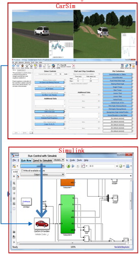
Table 1. Suspension parameters used in Simulation.

Parameter	Value/unite
Quarter car sprung mass (ms)	320 kg
Quarter car unsprung mass (mu)	40 kg
Suspension stiffness (ks)	18,000 N/m
Vertical stiffness of the tire (kt)	200,000 N/m
Suspension damper (cs)	1000 N·s/m
Maximum force output of actuator (Fmax)	1500 N
Maximum suspension deflection (Smax)	0.1 m

According to the theoretical analysis of Sections 4.1 and 4.2, the feedback control gains of H∞ controller and H∞ controller with two time scales can be obtained by solving the LMI in Matlab, such that

For H∞ controller: $K=-\left[1.1525,0.3082,2.6711,4.3032\right]\times {10}^5$For H∞ controller with two time scales: $\begin{array}{rl}{K}_s& =[2.6921\times {10}^4,1.4334\times {10}^3]\end{array}$ $\begin{array}{rl}{K}_f& =[-3.1399\times {10}^3,-1.0698\times {10}^3]\end{array}$In order to verify the effectiveness of the proposed two time scales H∞ controller, we select two highway driving conditions and off-road driving conditions from the special car simulation software Carsim to simulate more realistic road excitation conditions, and combine Simulink to achieve co-simulation.

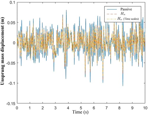
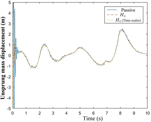
Case 1. Highway driving conditions road excitation: The suspension is excited by highway driving conditions road excitation, which comes from the Carsim data as shown in Figure 3. The comparison results of suspension states (the sprung mass displacement, sprung mass acceleration and unsprung mass displacement) produced by the three control methods (passive, H_∞ controller and H_∞ controller with two time scales) are shown in Figures 3–5, respectively. Compared with the passive suspension system, the active suspension system with the H_∞ controller and H_∞ controller with two time scales have the lower peak and less defection. Meanwhile, it should be pointed out that the proposed H_∞ controller with two time scales demonstrates smaller amplitude and faster transient convergence in terms of the sprung mass displacement, sprung mass acceleration and unsprung mass displacement than the general H∞ controller (Figure 6).

Figure 3. Highway driving conditions road excitation.

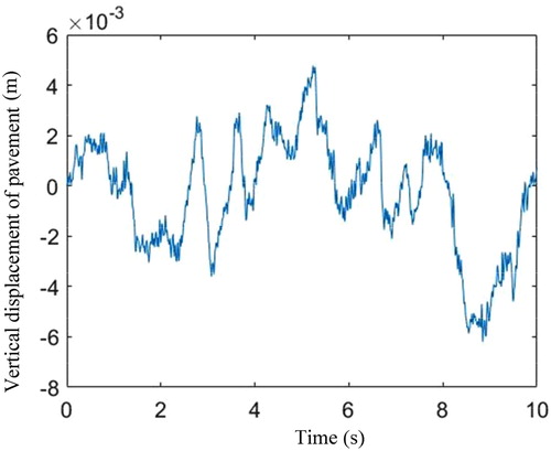
Figure 4. Sprung mass displacement on the highway driving conditions road excitation.

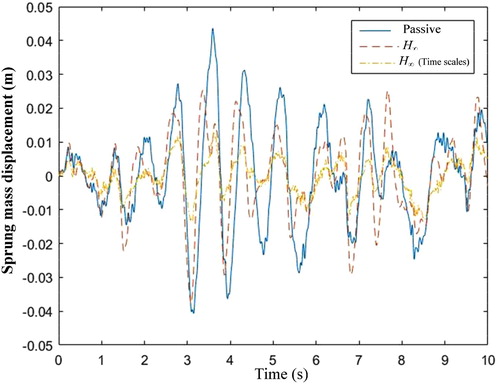
Figure 5. Sprung Mass acceleration on the highway driving conditions road excitation.

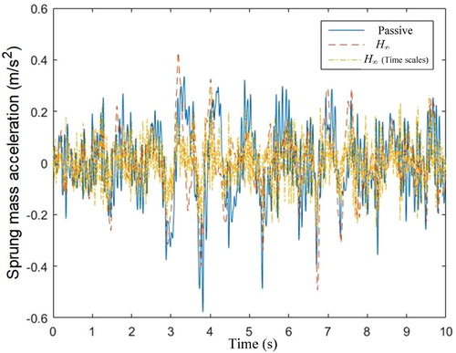
Figure 6. Unsprung mass displacement under the highway driving conditions road excitation.

Case 2. Off road excitation: In this case, we select the off-road driving conditions road excitation which comes from the Carsim data as shown in Figure 7. Other simulation parameters are the same as those used in case 1. As can be seen from Figures 8–10, the proposed two time scales H_∞ control method still shows better dynamic response performance compared with the general H_∞ control method. At the same time, it should be emphasized that different time scales property of the proposed H_∞ controller with two time scales makes the small oscillation of the suspension deflection response and the sprung mass acceleration even under severely bumpy off-road conditions.

Figure 7. Off-road driving conditions.

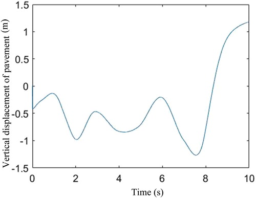
Figure 8. Sprung Mass displacement under the excitation of off-road conditions.

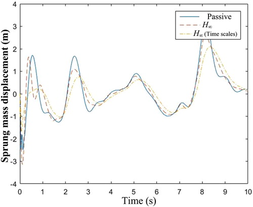
Figure 9. Mass acceleration under the excitation of off-road conditions.

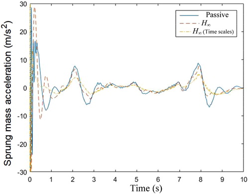
Figure 10. Mass displacement under the excitation of off-road conditions.

These aforementioned simulation results illustrate how the proposed H_∞ controller with two time scales for vehicle active suspension system provides better riding comfort and suspension movement performance. Moreover, it is shown that the decomposition into two sub-systems by the singular perturbation method is a useful means of designing the control law for an active suspension system for the quarter-car model. Since only two lower-order subsystems need to be considered, which is easy to apply various techniques. As a result, many methods for linear systems can be applied to design the control system for the active suspension with nonlinear characteristics, such as the H_∞ control method used in this paper.

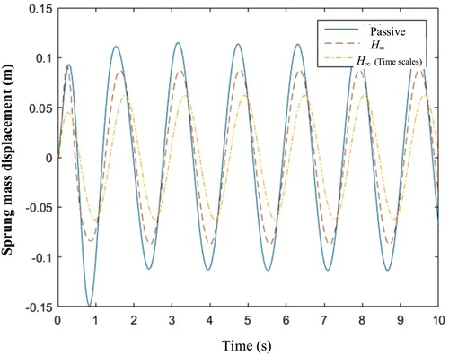
Case 3. Sinusoidal excitation: In this case, we select the sinusoidal excitation as shown in Figure 7. Other simulation parameters are the same as those used in cases 1 and 2.

As can be seen from Figures 11 and 12, the proposed two time scales H_∞ control method still shows better dynamic response performance compared with the general H_∞ control method.

Figure 11. Mass acceleration under sinusoidal excitation.

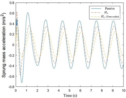
Figure 12. Mass displacement under sinusoidal excitation.

In addition, Root Mean Square (RMS) is used to further quantitatively compare the performance results of passive suspensions, active suspensions with H_∞ controller and two time scales H_∞ controller. Here, RMS is defined as $RMS=\sqrt{\frac{{\sum }_{i=1}^n{x}^2\left(i\right)}{n}}$where n is the number of the simulation steps, $x\left(i\right)$ is the corresponding state response at ith step.

RMS values for all of the states response both in aforementioned Cases 1–3 are listed in Table 2. It can be seen that the RMS values of the proposed two time scales H_∞ controller is the smallest, whether it is compared with passive suspension or with general H_∞ controller. This further shows that decoupling the suspension system and designing corresponding controllers according to the fast and slow subsystems can significantly improve the control effect, thus ensuring the smoothness and comfort of the vehicle.

Table 2. Corresponding RMS values under different excitations.

Parameter/(m/s^2)	Passive	H∞	H∞ (time scales)
Sprung mass acceleration (highway)	0.1124	0.0956	0.0657
Sprung mass acceleration (off road)	2.7895	2.5415	1.7592
Sprung mass acceleration (sinusoidal)	0.3175	0.2402	0.1583
Unsprung mass displacement (highway)	0.0119	0.0094	0.0042
Unsprung mass displacement (off road)	0.7715	0.6929	0.5768
Unsprung mass displacement (sinusoidal)	0.0689	0.0539	0.0384

6. Conclusions

In this paper, a state feedback H_∞ controller for quarter suspension systems is designed with the vertical acceleration as the optimization index and considering the constraints in terms of tire dynamic load, suspension dynamic travel and maximum output force constraints; Furthermore, in order to solve the coupling problem of vehicle handling stability and ride comfort, in view of the dual time scale characteristics of suspension system, the sprung and unsprung masses of the suspension system are decoupled by using the singular perturbation theory, and the joint H_∞ controller is designed for the fast subsystem and the slow subsystem, respectively. Compared with the commonly used H_∞ controller, the suspension systems with H_∞ controller in two time scales can better restrain the influence of road excitation transferring to the vehicle body, greatly improve the comfort of the vehicle, and make the inherent attribute constraints of the suspension system within its constraint range. The validity of the proposed approach is illustrated in terms of comparative simulations, which have been carried out based on a dynamic simulator built in a professional vehicle simulation software Carsim and Simulink. Future work will focus on practical validations of the proposed H_∞ controller with two time scales strategy in terms of a quarter-car active suspension test-rig with real hydro-pneumatic actuators.

Disclosure statement

No potential conflict of interest was reported by the author(s).

Additional information

Funding

This work was supported by National Natural Science Foundation of China: [Grant Number 51405436]; National Natural Science Foundation of China: [Grant Number 62073298]; Special Application for Key Scientific and Technological Project of Henan Province: [Grant Number 202102210290] [Grant Number 212102310454].

References

- Huang Y, Na J, Wu X, et al. Approximation-free control for vehicle active suspensions with hydraulic actuator. IEEE Trans Ind Electron. 2018;65:7258–7267.
- Ning D, Du H, Zhang N, et al. Controllable electrically interconnected suspension system for improving vehicle vibration performance. IEEE/ASME Trans Mechatron. 2020;25(2):859–871.
- Yuan Y, Ma Y, Xu J, et al. Full-period suspension force accurate modelling for a novel bearingless switched reluctance motor. Electron Lett. 2019;55(21):1119–1121.
- Zhu Q, Ding J, Yang M. LQG control based lateral active secondary and primary suspensions of high-speed train for ride quality and hunting stability. IET Control Theory Applic. 2018;12(10):1497–1504.
- Huang Y, Na J, Wu X, et al. Adaptive control of nonlinear uncertain active suspension systems with prescribed performance. ISA Trans. 2015;54:145–155.
- Song J, Niu Y, Zou Y. A parameter-dependent sliding mode approach for finite-time bounded control of uncertain stochastic systems with randomly varying actuator faults and its application to a parallel active suspension system. IEEE Trans Ind Electron. 2018;65(10):8124–8132.
- Huang Y, Na J, Wu X, et al. Robust adaptive control for vehicle active suspension systems with uncertain dynamics. Trans Inst Meas Control. 2016;40(4):1–13.
- Zheng X, Zhang H, Yan H, et al. Active full-vehicle suspension control via cloud-aided adaptive backstepping approach. IEEE Trans Cybern. 2020;50(7):3113–3124.
- Friedrichs K, Wasow W. Singular perturbations of non-linear oscillations. Duke Math J. 1940;13(3):367–381.
- Tikhonov A. Systems of differential equations containing small parameters in the derivatives. Matematicheskii Sbornik. 1952;31(73):575–586.
- O’Malley R. Singular perturbation methods for ordinary differential equations. New York (NY): Springer Verlag; 1991.
- Vasilieva A, Butuzov V, Kalachev L. The boundary function method for singular perturbation problems. Math Comput. 1996;65(215):1366–1368.
- Vasilieva A. On the development of singular perturbation theory at Moscow State University and elsewhere. SIAM Rev. 1994;36(3):440–452.
- Saksena V, O’reilly J, Kokotovic P. Singular perturbations and time-scale methods in control theory: survey 1976-1983. Automatica (Oxf). 1984;20(3):273–293.
- Mudita J, Nagar S, Mohanty R. PSO based reduced order modelling of autonomous AC microgrid considering state perturbation. Automatika. 2020;61(1):66–78.
- Li T, Wang S. Robust dynamic output feedback sliding mode control of singular perturbation systems. Jpn Soc Mech Eng. 1995;38(4):719–726.
- Ando Y, Suzuki M. Control of active suspension systems using the singular perturbation method. Control Eng Pract. 1996;4(3):287–293.
- Kim C, Ro P. Reduced-order modelling and parameter estimation for a quarter-car suspension system. Proc Inst Mech Eng Part D: J Automobile Eng. 2000;214:851–864.
- Carbinatto C. On the suspension isomorphism for index braids in a singular perturbation problem. Math Notebooks. 2007;8:173–198.
- Aghazadeh M, Zarabadipour H. Observer and controller design for half-car active suspension system using singular perturbation theory. Adv Mat Res. 2011;403-408:4786–4793.
- Paarya A, Zarabadipour H. Digital controller design for half-car active suspension system with singular perturbation theory. Adv Mat Res. 2011;403-408:4800–4805.
- Kokotovic P, O’Reilly J, Khalil H. Singular prturbation mthods in control: analysis and design. Orlando (FL): Academic Press, Inc.; 1986.
- Ahamd I, Abdurraqeeb A. H∞ control design with feed-forward compensator for hysteresis compensation in piezoelectric actuator. Automatika. 2016;57(3):691–702.
- Lien C, Vaidyanathan S, Yu K, et al. H∞ performance of continuous switched time-delay systems with sector and norm bounded nonlinearities. Int J Modell Ident Control. 2019;31(3):229–244.
- Shahad A, Safanah R, Ayman A. Improving the performance of medical robotic system using H∞ loop shaping robust controller. Int J Modell Ident Control. 2020;34(1):3–12.
- Wu J, Liu Z, Chen W. Design of a piecewise affine H∞ controller for MR semi-active suspensions with nonlinear constraints. IEEE Trans Control Syst Technol. 2019;27(4):1762–1771.
- Zhang J, Ding F, Zhang N, et al. A new SSUKF observer for sliding mode force tracking H∞ control of electrohydraulic active suspension. Asian J Control. 2020;22(2):761–778.
- Na J, Huang Y, Wu X, et al. Active adaptive estimation and control for vehicle suspensions with prescribed performance. IEEE Trans Control Syst Technol. 2018;26(6):2063–2077.
- Dhananjay K, Kumar S. Modeling and simulation of quarter car semi active suspension system using LQR controller. Adv Intell Syst Comput. 2014;1:441–448.
- BalaMurugan L, Jancirani J. An investigation on semi-active suspension damper and control strategies for vehicle ride comfort and road holding. Proc IMechE Part I: J Syst Control Eng. 2012;226(8):1119–1129.
- Yury V, Luis A. Advanced H∞ control towards nonsmooth theory and applications. New York (NY): Birkhäuser; 2014.
- Kokotovic P, O’Malley J, Sannuti P. Singular perturbations and order reduction in control theory–an overview. Automatica (Oxf). 1976;12(2):123–132.
- Kokotovic P. Subsystem, time scales and multimodeling. Automatica (Oxf). 1981;17(16):789–795.