A comparative study of DC servo motor parameter estimation using various techniques

Abstract

A lot of research is being carried out on the Direct Current (DC) servo motor systems due to their excessive applications in various industrial sectors owing to their superior control performance. Parameters of the DC servo motor systems to be used in the simulation software are usually unknown or change with time and have to be determined accurately for obtaining the precise simulation response. In this paper, three different estimation techniques for multi-domain DC servo motor model parameters are discussed namely the Compare Coefficient Method, MATLAB Parameter Estimation Toolbox, and System Identification Toolbox. The paper performs a comparison of these methods to identify the one that gives the most accurate results. Experimental data has been used for the comparison of the estimated response from the techniques. The results show that the parameters obtained from the parameter estimation method give the most accurate simulation results with the least error against the experimental results. The study is significant for guiding researchers to prefer this method for estimation purposes of DC servo motor simulation model parameters. The presented technique, i.e. parameter estimation technique,  is relatively less complex and requires less computational cost as compared to other techniques found in the literature.

KEYWORDS:

• DC servo motor
• Parameter estimation
• Design optimization toolbox
• Parameter estimation toolbox
• DC motor first-principle model
• Comparing coefficient method

1. Introduction

Direct Current (DC) motors are used in different fields of consumer electronics, industries, and robotics. Parameters of DC motor play an important role in achieving high performance in simulation models. Parameters vary with time due to the depreciation and aging effect which reduces performance, therefore, to overcome this problem, motor parameters should be updated and different techniques have been used for this purpose [1]. Motion Control Techniques (MCT) have been tremendously developed in the last decade. In 1990, Advanced Motion Control based first IEEE International workshop was held, which highlighted the physical examination of Motion Control (MC). MC systems became dominant in velocity, position, force, and acceleration control. Industrial robotic systems’ performance is measured by control of force and position. DC servomotors are frequently used to attain accurate torque and position control. Furthermore, due to the low cost, outstanding control performance, and simple structure, their usage is spreading in the robotics field [2,3].

DC Servo motors have  been proved useful for industrial MC systems due to their good features of less noise, energy efficiency, low manufacturing cost, fast response, torque to inertia ration, little volume, and high accuracy [4–6]. In industries, servo motor systems are extensively utilized as actuators [7], which include permanent-magnet synchronous motor [8], direct current brushless motor [8], and direct current brushed motor [9]. Two types of actuators are used for vehicle systems, first one is used in electro-pneumatic systems or electro-hydraulic systems called solenoid valve [10,11] while the second one is used in the electromechanical system which is termed as direct current servo motor systems or DC motor [12,13].

Different advanced techniques self-tuning controller, model reference adaptive controller, sliding mode controller (SMC), adaptive backstepping control, fuzzy control, and genetic algorithm have been implemented for the improvement of the system's performance [14–16]. The schematic diagram of the DC servo motor is shown in Figure 1. Controller parameter tuning depends upon system physical parameters. Hence, recognition of system physical parameters accuracy is essential. Some fixed parameters (resistance of armature Ra, the inductance of armature La, and Ke back-emf constant) are considered for DC motor. Because of magnetic effects, the torque constant may change, when the direct current motor is in operation mode. Also with the removal of loads or additional loads to the rotary shaft, inertia J of motor changes [17].

Figure 1. Schematic diagram of the DC servo motor [16].

This literature review shows that all the previously developed methods are built upon parameter knowledge of the accurate model. Still, because of manufacturing discrepancy and different application schemes disturbances, unknown parameters and backlashes surely occur in the DC motor servo systems. Consequently, with previously mentioned uncertainties it seems still tough to control DC motor servo systems. It is noted that adaptive control can handle different types of system uncertainties [18,19], which includes parametric uncertainties [20–22], non-smooth nonlinear uncertainty [23–25], time-delay [26–28], and disturbances that are not known [29,30]. A PID-type feedback controller with adaptive gain parameters was introduced for backlash nonlinearity, for position control [31]. In actuality, with the advancement and betterment of manufacture highly precise actuators are needed in vehicle applications when the backlashes and gaps are very small. As a result of the above discussion, we can say that the main uncertainties are disturbances and unknown parameters, not backlashes. In the future an indirect method of comparing coefficients can be used also online parameter estimation of DC motor can be done without the need to have information about parameters in advance. Further, controller parameters can be estimated from artificial intelligent techniques. Whenever load changes occur, this method will improve the system response in real-time. Scientists and Engineers of different fields and industries have good knowledge about the advantages of modelling dynamic systems. They can use test-data-based methods or methods of first-principles mathematics. First-principles models give understanding about the behaviour of the system, but at the same time reduce accuracy. Data-driven models give good accuracy, but they provide a limited understanding of system physics. In this paper five parameters (Ra, La, Km, J, and B) are used for the model of the motor.

There has been a lot of studies done on parameter estimation techniques in general. In [32], the authors propose a new parameter estimation approach based on the Dynamic Regressor Extension and Mixing (DREM) method. When compared to gradient-based and least-squares estimators, this method has been shown to perform better. The DREM strategy's performance has been improved further in [33,34]. [35] describes how signal injection techniques may be used to reduce the complexity of parameter estimation-based observers. This approach is used to create a sensorless controller for magnetic levitation devices, and the findings are confirmed using numerical simulations. [36] describes a new technique for partial state identification of nonlinear systems based on parameter identification. In [37], an adaptive parameter estimation approach for nonlinear systems with unknown time-varying parameters was introduced. The adaptive method estimates parameters using input and output data and is validated using gradient-based and least-squares techniques. Furthermore, the method's resilience is demonstrated experimentally on a roto-magnet plant with limited disturbance.

The techniques presented in the literature are much complex and require huge computational cost making these unattractive for common DC servo motor parameter estimation purposes. The contributions of the paper are summarized as: (1) the first-principle model of DC servo motor is developed and comparing coefficients method has been used to determine the system parameters. (2) The parameter estimation toolbox has been used to estimate the parameters and validate the response of the system. (3) System identification toolbox has been used to estimate parameters. (4) comparison of the three methods has been carried out to select the best option for such applications. Experimental data has been used for the comparison of the estimated response from the techniques. The results show that the parameters obtained from the parameter estimation method give the most accurate simulation results with the least error against the experimental results. The study is significant for guiding researchers to prefer this method for estimation purposes of DC servo motor simulation model parameters. The study is novel with respect to literature that no such comparative study was found justifying the superior performance of parameter estimation toolbox method for estimating the parameters of a DC servomotor.

The next sections are organized in the following way, Section II discusses the research methodology, Section III presents results with discussion and the comparison of two methods. Section IV concludes the document.

2. Research methodology

A list of parameters with symbols used in the study for estimation is shown in Table 1.

Table 1. List of parameters and symbols for DC servo motor.

Parameter	Abbreviation	Units
Moment of Inertia	$J_m$	$\mathrm{Kg}.{\mathrm{m}}^2$
Back EMF constant	$K_b$	$\text{Volts}/\text{rad}/\text{sec}$
Torque Constant	$K_t$	$\text{N}\text{.m}/\text{A}$
Frictional Constant	$B_m$	$\text{N}\text{.m}/\text{rad}/\text{sec}$
Electric Resistance	$R_a$	Ω
Electric Inductance	$L_a$	$\text{H}$
Armature Current	$I_a$	$\text{A}$
Angle of motor shaft	$\theta$	$\text{rad}$
Developed Torque	$T_m$	$\text{N}\text{.m}$
Load Torque	$T_l$	$\text{N}\text{.m}$
Back EMF	$E_b$	$\text{Volts}$
Armature Voltage	$E_a$	$\text{Volts}$

2.1. Modelling using comparing coefficient method

In this method, we estimate the parameters of a DC servo motor using the DC servo motor subsystem. The model of DC motor is formulated with its mechanical and electrical subsystems using Simscape Driveline and Electrical line. Input voltage ($V$) is applied to the motor and output measured is the motor shaft’s angular position, $\theta$ as shown in Figure 2.

Figure 2. DC servo motor subsystem [38].

Dynamic parameters of Servo motor can be estimated using the following equations given below: (1) $\begin{array}{rl}{E}_a(s)& =R_a{I}_a(s)+L_{a}s{I}_a(s)+E_b(s)\end{array}$(1) (2) $\begin{array}{rl}{T}_m& =K_t{I}_a(s)\end{array}$(2) (3) $\begin{array}{rl}{T}_m& =(J_m{s}^2+D_{m}s)\theta (s)\end{array}$(3) (4) $\begin{array}{rl}{E}_b(s)& =K_{b}s\theta (s)\end{array}$(4)

2.2. Modelling using parameter estimation technique

In this method, practical measurements from a real DC servo motor are first taken. We then need to identify and specify parameters to estimate, starting with some initial guess. After feeding this data into the model, parameter values are approximated using a suitable approximation algorithm from Parameter Estimation Toolbox in Simulink. 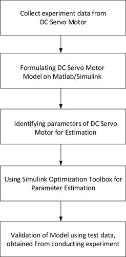Five parameters: Frictional constant $B_m$, Moment of Inertia $J_m$, Torque Constant $K_t$, Inductance $L_a$ and Resistance $R_a$ of servo motor are chosen and are loaded in the Parameter Estimation tool. Practically, measured data is also loaded for validation of the model. The next step is to plot both measured and simulated data to see how much it matches current DC Servo Motor’s data. If the simulation does not match the measured data, model parameters need to be estimated again. The parameter estimation tool will continue to iterate parameter values until estimation converges or terminates. Plots of measured and simulated data can be overlaid to show how successful is the estimation process. After completion of parameter approximation, we need to validate our results using other test data sets that can be measured from the real DC servo motor. The steps involved in the evaluation of the parameter estimation of DC Servo Motor using the parameter estimation toolbox are shown in Figure 3.

Figure 3. Shows steps involved in parameter estimation of DC servo motor.

2.3. Modelling using system identification technique

Another technique to estimate parameters for DC Servo Motor is using System Identification Toolbox if we have measured input and output data. In this study, the estimation and validation input and output data were obtained from MATLAB DC Servo Motor Example [38].

3. Results and discussion

DC Servo Motor system is developed in Simulink using the Simscape Driveline and Simscape Electrical as shown in Figure 4 which shows Simulink model of DC Servo motor used for estimation of motor parameters.

Figure 4. Shows the Simulink model of DC servo motor [38].

3.1. Parameter estimation using comparing coefficient method

Before starting the estimation process, we need to know system equations that physically represent DC Servo Motor. The dynamic parameters of the Servo motor can be estimated using the Equations (1) to (4). By taking Laplace Transform of all the above equations and after simplifying, the following transfer function is obtained: (5) $G(s)=\frac{\theta (s)}{E_a(s)}=\frac{{K_t}^{-1}}{s[(R_a+s{L}_a)((J_m+D_m)+{K_t}^2]}$(5) Expanding denominator we get, (6) $\begin{array}{rl}G(s)& =\frac{\theta (s)}{E_a(s)}=\frac{K_t}{\begin{array}{c}(J_m{L}_a)s^3+(R_a{J}_m+Dm{L}_a)s^2\\ +(D_m{R}_a+{K_t}^2)s\end{array}}\end{array}$(6) After finding Values of $K,T_{p1}$ and $T_{p2}$, we can find numerical values of motor parameters by evaluating Equation (6) and process model transfer function Equation (8). (7) $\begin{array}{rl}G(s)& =\frac{\theta (s)}{E_a(s)}=\frac{{K_t}^{-1}}{\begin{array}{c}(J_m{L}_a)s^3+(R_a{J}_m+Dm{L}_a)s^2\\ +(D_m{R}_a+{K_t}^2)s\end{array}}\end{array}$(7) (8) $\begin{array}{rl}P(s)& =\frac{K}{s(1+T_{p1}s)(1+T_{p2}s)}\end{array}$(8) (9) $\begin{array}{rl}P(s)& =\frac{K}{T_{p1}{T}_{p2}{s}^3+(T_{p1}+T_{p2})s^2+s}\end{array}$(9)

Evaluating coefficients of (6) and (8), we get (10) $\begin{array}{rl}{T}_{p1}{T}_{p2}& =J_m{L}_a\end{array}$(10) (11) $\begin{array}{rl}{R}_a{J}_m+Dm{L}_a& =T_{p1}+T_{p2}\end{array}$(11) (12) $\begin{array}{rl}1& =D_m{R}_a+{K_t}^2\end{array}$(12) The value of $R_a$ is assumed to find other parameters by solving and putting values in other equations. We get the following values: $\begin{array}{rl}{J}_m& =9.027\text{e}-3\mathrm{\Omega }\end{array}$ $\begin{array}{rl}{K}_t& =4.943\text{e}-3(\text{N}\text{.m}/\text{A})\end{array}$ $\begin{array}{rl}{D}_m& =0.518(\text{N}\text{.m}/\text{rad}/\text{sec})\end{array}$ $\begin{array}{rl}{R}_a& =1.93\mathrm{\Omega }\end{array}$ $\begin{array}{rl}{L}_a& =2.348\text{e}-3\text{H}\end{array}$The estimated values are about 90% closer to the actual measurements.

3.2. Parameter estimation using parameter estimation toolbox

Estimation of the Motor parameter is done using the Parameter Estimation toolbox. Pre-loaded data from the practical experiment is already available in this project. Experimental data can also be loaded from MATLAB variables, MAT files, Excel, or comma-separated-value files. The next task is to select parameters that are planned to be estimated for the DC Servo motor. Five Parameters are chosen Frictional constant $B_m$, Moment of Inertia $J_m$, Torque Constant $K_t$, Inductance $L_a$ and Resistance $R_a$. We set the initial values of these parameters, as mentioned in the datasheet of DC Servo Motor. The range of these parameters from zero to infinity is also defined. The initial values of these parameters are shown in Table 2.

Table 2. Shows the initial values of these parameters.

Parameter	Initial parameter values	Units
$J_m$	5.7e-7	$\mathrm{Kg}.{\mathrm{m}}^2$
$K_t$	0.0134	$\text{N}\text{.m}/\text{A}$
$D_m$	0.008	$\text{N}\text{.m}/\text{rad}/\text{sec}$
$R_a$	1.9	Ω
$L_a$	6.5e-5	$\text{H}$

We plot the model response of the experimental data along with the simulated data. It is found that the simulation data does not match with practically measured data, showing that model parameters need to be tuned as shown in Figure 5.

Figure 5. Shows the difference between model plot response of measured and simulated data.

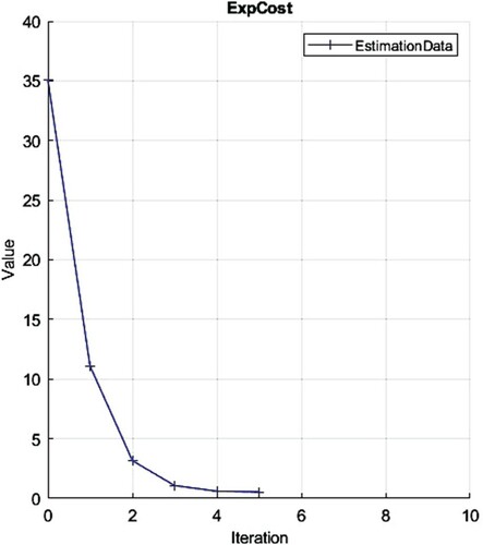
Next, we add a plot of Parameter Trajectory, which shows how parameter values change during the estimation process. Estimation is done based on a cost function. For this experiment, the cost function of Sum Squared Error is selected. Next, the Estimation process is started, it keeps iterating parameter values until estimation converges and stops. Once the process terminates, we obtain the estimation progress report featuring the iteration number and values from the cost function. The convergence steps of the algorithm are shown in Table 3.

Table 3. Estimation progress report.

Iteration	F- Count	Estimation data
0	11	35.0694
1	22	11.0708
2	33	3.1677
3	44	1.0813
4	55	0.6050
5	66	0.5462

The cost function minimization plot is shown in Figure 6 to show the progress of the algorithm after each iteration till convergence.

Figure 6. Cost function used for estimation process.

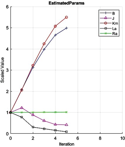
The parameter trajectory plot for various parameters to be estimated is shown in Figure 7 to show the progress to approach their final values.

Figure 7. Parameter trajectory plot of DC servo motor.

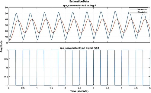
The model fit plot of the estimated data with measured data is shown in Figure 8 which shows the accuracy of the technique after few iterations.

Figure 8. Model plot response of simulated data.

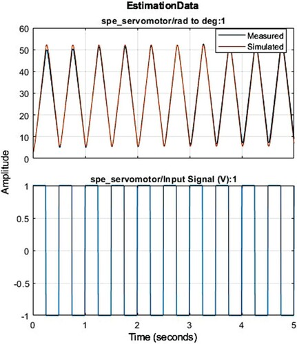
A successful estimation should not match only the experimental data set but also other test data, which is collected from a practical experiment. The Validation data set is pre-loaded for this experiment. It is observed from simulation results that the model plot response of the test dataset accurately matches with the simulated data. The results obtained from this method are about 99% closer to the actual measurements proving its greater accuracy.

3.3. Parameter estimation using system identification toolbox

We obtain two measured data sets for estimation and validation. min and mout are measured input and output that will be used for estimation and vin and vout  are measured input and output that will be used for validation of the model. The next step is to convert input and output data in MATLAB workspace to iddata variable. This can be done by using the following command: $\text{data}=\text{iddata}(\text{output},\text{input},\text{Ts})$where Ts is a sampling time that is 0.005 s.

Two iddata objects; mdata and vdata are set. These two variables are added to the system identification toolbox for the estimation of the model. We modify mdata object and select input and output values from 0 to 2 s with Ts = 0.005 s.

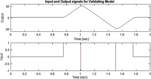
The following steps are repeated for vdata and vdatae is obtained with validation input and outputs ranging from 0 to 2 s. The plots of input and output signals for the estimation and validation are shown in Figures 9 and 10.

Figure 9. Measured input and output data plot, used for estimation.

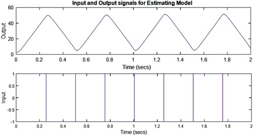
Figure 10. Measured input and output data plot, used for validation.

Next, we select a process model that will depict the dynamics of our DC Servo Motor which is two real poles-based system with an integrator in series to estimate gain and poles values. The values of $K,T_{p1}$ and $T_{p2}$ are estimated. The plots of the process model with estimation and validation data are shown in Figures 11 and 12. It is seen from the results that both validation and estimation data map each other accurately up to  96%.

Figure 11. Process model P2 fits estimation data up to 96%.

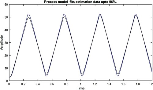
Figure 12. Process model P2 fits validation data up to 94%.

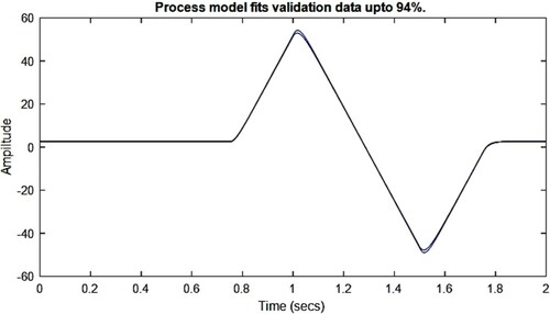
3.4. Comparison of presented techniques

The paper presented a comparison of the three popular methods for estimating the parameters of the DC servo motor system. The conventional method using the comparing coefficient method is an easy one but lacks accuracy in terms of achieving experimental results. The second method using the parameter estimation toolbox provided the highest accuracy. The third method was the system identification technique that provided an accurate response less than the parameter estimation toolbox. Therefore, the recommended method from this study is the parameter estimation toolbox (Table 4).The parameter estimation technique is also relatively less complex and requires less computational cost as compared to other techniques found in the literature mentioned earlier.

Table 4. Comparison of the parameter estimation techniques.

Technique	Accuracy
Comparing Coefficient Method	90%
Parameter Estimation Toolbox	99%
System Identification Toolbox	94-96%

4. Conclusion

This paper presented three estimation techniques for multi-domain DC servo motor model parameters namely the Compare Coefficient Method, MATLAB Parameter Estimation Toolbox, and System Identification Toolbox. The paper also performed a comparison of these methods to identify the one that gives the most accurate results. The results showed that the parameters obtained from the parameter estimation method give the most accurate simulation results with the least error against the experimental results. The study is significant for guiding researchers to prefer this method for estimation purposes of DC servo motor simulation model parameters.

Future directions may include the inclusion of different parameters other than these for better results. Advanced neural network or fuzzy-based or combination of these estimation methods may also be tested for performance comparison in future studies with experimental verification like Hardware-in-the Loop technique.

Acknowledgements

The authors would like to thank to colleagues for suggestions to improve the paper quality.

Disclosure statement

No potential conflict of interest was reported by the author(s).

References

- Usman HM, Mukhopadhyay S, Rehman H. Permanent magnet DC motor parameters estimation via universal adaptive stabilization. Control Eng Pract. Sep. 2019;90:50–62. doi:https://doi.org/10.1016/j.conengprac.2019.06.006.
- Kommuri SK, Defoort M, Karimi HR, et al. A robust observer-based sensor fault-tolerant control for PMSM in electric vehicles. IEEE Trans Ind Electron. Dec. 2016;63(12):7671–7681. doi:https://doi.org/10.1109/TIE.2016.2590993.
- Das D, Kumaresan N, Nayanar V, et al. Development of BLDC motor-based elevator system suitable for DC microgrid. IEEE/ASME Trans Mechatron. Jun. 2016;21(3):1552–1560. doi:https://doi.org/10.1109/TMECH.2015.2506818.
- Chaoui H, Khayamy M, Aljarboua AA. Adaptive interval type-2 fuzzy logic control for PMSM drives with a modified reference frame. IEEE Trans Ind Electron. May 2017;64(5):3786–3797. doi:https://doi.org/10.1109/TIE.2017.2650858.
- Li P, Zhu G. Robust internal model control of servo motor based on sliding mode control approach. ISA Trans. Oct. 2019;93:199–208. doi:https://doi.org/10.1016/j.isatra.2019.03.021.
- Xie Y, Tang X, Song B, et al. Data-driven adaptive fractional order PI control for PMSM servo system with measurement noise and data dropouts. ISA Trans. Apr. 2018;75:172–188. doi:https://doi.org/10.1016/j.isatra.2018.02.018.
- Shi D, Xue J, Zhao L, et al. Event-triggered active disturbance rejection control of DC torque motors. IEEE/ASME Trans Mechatron. Oct. 2017;22(5):2277–2287. doi:https://doi.org/10.1109/TMECH.2017.2748887.
- Mwasilu F, Nguyen HT, Choi HH, et al. Finite set model predictive control of interior PM synchronous motor drives with an external disturbance rejection technique. IEEE/ASME Trans Mechatron. Apr. 2017;22(2):762–773. doi:https://doi.org/10.1109/TMECH.2016.2632859.
- Ghosh M, Panda GK, Saha PK. Analysis of chaos and bifurcation due to slotting effect and commutation in a current discontinuous permanent magnet brushed DC motor drive. IEEE Trans Ind Electron. Mar. 2018;65(3):2001–2008. doi:https://doi.org/10.1109/TIE.2017.2745446.
- Meng F, Chen H, Zhang T, et al. Clutch fill control of an automatic transmission for heavy-duty vehicle applications. Mech Syst Signal Process. Dec. 2015;64–65:16–28. doi:https://doi.org/10.1016/j.ymssp.2015.02.026.
- Song X, Sun Z. Pressure-based clutch control for automotive transmissions using a sliding-mode controller. IEEE/ASME Trans Mechatron. Jun. 2012;17(3):534–546. doi:https://doi.org/10.1109/TMECH.2011.2106507.
- Gao B, Chen H, Liu Q, et al. Position control of electric clutch actuator using a triple-step nonlinear method. IEEE Trans Ind Electron. Dec. 2014;61(12):6995–7003. doi:https://doi.org/10.1109/TIE.2014.2317131.
- Li G, Tsang KM. Concurrent relay-PID control for motor position servo systems. 2007.
- Bindu R, Namboothiripad MK. Tuning of PID controller for DC servo motor using genetic algorithm. 2012.
- Wang X, Wang W, Li L, et al. Adaptive control of DC motor servo system with application to vehicle active steering. IEEE/ASME Trans Mechatron. Jun. 2019;24(3):1054–1063. doi:https://doi.org/10.1109/TMECH.2019.2906250.
- Ohnishi K, Katsura S, Shimono T. Motion control for real-world haptics. IEEE Ind Electron Mag. Jun. 2010;4(2):16–19. doi:https://doi.org/10.1109/MIE.2010.936761.
- Ma H, Zhou Q, Bai L, et al. Observer-based adaptive fuzzy fault-tolerant control for stochastic nonstrict-feedback nonlinear systems with input quantization. IEEE Trans Syst Man Cybern Syst. Feb. 2019;49(2):287–298. doi:https://doi.org/10.1109/TSMC.2018.2833872.
- Liu Z, Chen C, Zhang Y. Decentralized robust fuzzy adaptive control of humanoid robot manipulation with unknown actuator backlash. IEEE Trans Fuzzy Syst. Jun. 2015;23(3):605–616. doi:https://doi.org/10.1109/TFUZZ.2014.2321591.
- Fesharaki SJ, Kamali M, Sheikholeslam F. Adaptive tube-based model predictive control for linear systems with parametric uncertainty. IET Control Theory Appl. Aug. 2017;11(17):2947–2953. doi:https://doi.org/10.1049/iet-cta.2017.0228.
- Long J, Wang W, Huang J, et al. Distributed adaptive control for asymptotically consensus tracking of uncertain nonlinear systems with intermittent actuator faults and directed communication topology. IEEE Trans Cybern. 2019: 1–12. doi:https://doi.org/10.1109/TCYB.2019.2940284.
- Guo Q, Yin J, Yu T, et al. Saturated adaptive control of an electrohydraulic actuator with parametric uncertainty and load disturbance. IEEE Trans Ind Electron. Oct. 2017;64(10):7930–7941. doi:https://doi.org/10.1109/TIE.2017.2694352.
- Lai G, Liu Z, Zhang Y, et al. Asymmetric actuator backlash compensation in quantized adaptive control of uncertain networked nonlinear systems. IEEE Trans Neural Netw Learn Syst. Feb. 2017;28(2):294–307. doi:https://doi.org/10.1109/TNNLS.2015.2506267.
- Zhu Y, Su H, Krstic M. Adaptive backstepping control of uncertain linear systems under unknown actuator delay. Automatica. Apr. 2015;54:256–265. doi:https://doi.org/10.1016/j.automatica.2015.02.013.
- Arefi MM, Zarei J, Karimi HR. Adaptive output feedback neural network control of uncertain non-affine systems with unknown control direction. J Franklin Inst. Aug. 2014;351(8):4302–4316. doi:https://doi.org/10.1016/j.jfranklin.2014.05.006.
- Zhou J, Wen C, Zhang Y. Adaptive backstepping control of a class of uncertain nonlinear systems with unknown backlash-like hysteresis. IEEE Trans Autom Control. Oct. 2004;49(10):1751–1759. doi:https://doi.org/10.1109/TAC.2004.835398.
- Lu Z, Huang P, Liu Z. Predictive approach for sensorless bimanual teleoperation under random time delays with adaptive fuzzy control. IEEE Trans Ind Electron. Mar. 2018;65(3):2439–2448. doi:https://doi.org/10.1109/TIE.2017.2745445.
- Zhao X, Yang H, Karimi HR, et al. Adaptive neural control of MIMO nonstrict-feedback nonlinear systems with time delay. IEEE Trans Cybern. Jun. 2016;46(6):1337–1349. doi:https://doi.org/10.1109/TCYB.2015.2441292.
- Zhou J, Wang W. Adaptive control of quantized uncertain nonlinear systems. IFAC-PapersOnLine. Jul. 2017;50(1):10425–10430. doi:https://doi.org/10.1016/j.ifacol.2017.08.1970.
- Manikandan S, Kokil P. Stability analysis of network-controlled DC position servo system with time-delay. Automatika. Apr. 2021;62(2):163–171. doi:https://doi.org/10.1080/00051144.2020.1800265.
- Salas-Peña O, Castañeda H, de León-Morales J. Robust adaptive control for a DC servomotor with wide backlash nonlinearity. Automatika. Jan. 2015;56(4):436–442. doi:https://doi.org/10.1080/00051144.2015.11828657.
- Xudong Y. Nonlinear adaptive learning control with disturbance of unknown periods. IEEE Trans Autom Control. May 2012;57(5):1269–1273. doi:https://doi.org/10.1109/TAC.2011.2173414.
- Ortega R, Praly L, Aranovskiy S, et al. On dynamic regressor extension and mixing parameter estimators: two Luenberger observers interpretations. Automatica. Sep. 2018;95:548–551. doi:https://doi.org/10.1016/j.automatica.2018.06.011.
- Aranovskiy S, Bobtsov A, Ortega R, et al. Performance enhancement of parameter estimators via dynamic regressor extension and mixing*. IEEE Trans Autom Control. Jul. 2017;62(7):3546–3550. doi:https://doi.org/10.1109/TAC.2016.2614889.
- Belov A, Aranovskiy S, Ortega R, et al. Enhanced parameter convergence for linear systems identification: The DREM approach*. 2018 European Control Conference (ECC); 2018 Jun. p. 2794–2799. doi:https://doi.org/10.23919/ECC.2018.8550338.
- Yi B, Ortega R, Zhang W. Relaxing the conditions for parameter estimation-based observers of nonlinear systems via signal injection. Syst Control Lett. Jan. 2018;111:18–26. doi:https://doi.org/10.1016/j.sysconle.2017.10.011.
- Ortega R, Bobtsov A, Pyrkin A, et al. A parameter estimation approach to state observation of nonlinear systems. Syst Control Lett. Nov. 2015;85:84–94. doi:https://doi.org/10.1016/j.sysconle.2015.09.008.
- Na J, Xing Y, Costa-Castelló R. Adaptive estimation of time-varying parameters with application to roto-magnet plant. IEEE Trans Syst Man Cybern Syst. Feb. 2021;51(2):731–741. doi:https://doi.org/10.1109/TSMC.2018.2882844.
- DC Servo Motor Parameter Estimation – MATLAB & Simulink – MathWorks India. [cited 2020 Jan 16]. https://in.mathworks.com/help/sldo/examples/dc-servo-motor-parameter-estimation.html?s_tid=mwa_osa_a.