Stabilization of the cart-inverted-pendulum system using trivial state-feedback to output-feedback control conversion

Abstract

A new linear observer-free output-feedback controller with five adjustable parameters is proposed to stabilize the cart-inverted-pendulum system (CIP) at the unstable equilibrium point. The controller architecture is deduced from a trivial conversion of the linear state-feedback controller that is obtained using a two-step method. First, based on a set of cart change variables, a slightly modified state-feedback controller is developed. Then, the output-feedback controller is obtained through the judicious combination of the cart step reference input internal model and a convenient open-loop state estimator with the above modified state-feedback controller. The local stability of the output-based control system is conducted using the signature formulas method to get simplified conditions. A partial single parameter tuning method and optimal global single parameter tuning method are proposed for adjusting the controller gains to maximize a new efficiency-based objective function. Numerical simulations are first conducted to reveal the simplicity of output-feedback controller design using the partial tuning method, where the state-feedback gains are assumed to be known. Then, an optimal output-feedback controller is designed using the global tuning method. The proposed output-feedback controller is equivalent in terms of performance efficiency to the best five-parameter output-feedback two PID controller.

KEYWORDS:

• Cart-inverted-pendulum (CIP) system
• static state-feedback control
• dynamic output-feedback control
• signature formulas stability analysis
• output-feedback two PID controller

1. Introduction

Being an under-actuated mechanical system and inherently open-loop unstable with non-minimum phase and fourth-order highly nonlinear dynamics, the cart-inverted-pendulum (CIP) system provides many challenging control problems to standard and modern control techniques [1], especially in the absence of velocity measurements and in the presence of system uncertainties, measurement noises, and external disturbances. In the context of the CIP system stabilization, driving the cart from an initial position to a final destination while keeping the pendulum erected in the upright position during such movement is a well-studied problem, and many linear [2–6] and nonlinear [10–14,20,21] controllers, including state-feedback controllers (SFC), observer-based output-feedback controllers (OBC) and observer-free output-feedback controllers (OFC), have been proposed to solve it. However, achieving this task efficiently with reduced smooth control effort and simple parameter-tuning output-feedback control schemes is a subject that still needs more investigation.

Based on the linearized system dynamics using the standard pendulum small-angle approximations: $\sin x_1\approx x_1$ and $\cos x_1\approx 1$, the fact that the obtained linear model is controllable, and the assumption of accessibility of the state vector, many linear SFC, including Two Proportional and Derivative (TPD) [2–4] and Two Proportional–Integral–Derivative (TPID) [4–6] controllers, have been proposed to stabilize the equilibrium. The under-actuating property of the CIP system and the interaction that exists between the pendulum and cart dynamics make it useful, if not necessary, to combine at least two structures in the same controller to solve the stabilization problem [5,6]. Such a combination leads to an increase in the control parameters and consequently complicates the tuning parameter problem. The exigent control system requirements have led to the application of different controller tuning methods, such as the pole placement design [4], the Linear Quadratic Regulator (LQR) [4], and the optimization methods [7,8]. The comparison of the full-state-feedback controllers has been conducted in [9] and the main issues when using the above tuning methods are respectively: how to choose the optimal pole locations in the s-plane, the LQR criterion matrix gains, and the form of the objective function to be optimized?

Considering that the CIP system velocities are not (accurately) measured and the system, which is also subject to uncertainties, disturbances, and measurement noises, is observable with the set of position outputs, several (nonlinear) OBC and OFC have been proposed to stabilize the CIP system while addressing these difficulties to some extent. In [10], an extended high-gain OBC with dynamic inversion and multi-time-scale structure was proposed to deal with uncertainties and parameter tuning difficulties. The stability analysis for the multi-time-scale structure was carried out using singular perturbation methods. The conducted numerical simulations showed that the above proposed nonlinear OBC recovers the performance of its associated nonlinear SFC when using some small enough time-scale control parameters and demonstrated a large region of attraction of the equilibrium. Practical experiments have also been conducted but with initial pendulum angles in the neighbourhood of the upright configuration to prevent the exceeding of the cart bounded tracks and the physical limitations of the motor torque. In [11], a nonlinear OBC was proposed to deal with the pendulum input disturbance rejection and the CIP state velocity variable estimations. To achieve the nonlinear controller design, a simplified CIP model was considered, in which the pendulum and cart second-order dynamics are only coupled with the input control. The velocity estimation was done by the extended Kalman filter. Local asymptotic stability of the closed-loop CIP system was verified through the application of the eigenvalue analysis on the linearized CIP system. In [12], the author introduced a nonlinear state observer in a static linear SFC loop to design an OBC. As such introduction may adversely affect the stability robustness of the system, i.e. the gain and phase margins, LTR (Loop Transfer Recovery) technique has been used to redesign the observer in such a way as to shape the loop gain properties to approximate, to some extent, those of LQR. The feasibility of the observer-based method was demonstrated in [11] through practical experimentation and in [12] through numerical simulations. Other OBC applied to the CIP system can be found in [13,14].

With the introduction of observers that have their tuning parameters, the (multi-structure) controller design problem becomes again harder. Of course, a reduced-order observer can be used to estimate the unavailable velocities and the set of tuning parameters will be reduced; but if the CIP system position measurements are contaminated by noise, sensitivity to measurement noise becomes an issue that cannot be ignored. To stabilize the CIP system, OFC that processes directly the accessible CIP system positions, i.e. the pendulum angle and the cart position, without the (explicit) estimation of the state variable, is a promising approach. The progress in solving (linear and nonlinear) output-feedback regulation problems, has made it possible to design such an OFC for a wide class of systems to ensure, in addition to closed-loop stability, asymptotic tracking, and disturbance rejection for a class of reference inputs and disturbances. Some of the seminal works on the subject are given in [15] and [16]. The book [17] that addresses this general topic gives a rigorous formulation of the problem with its solvability conditions in terms of the existence of a solution to a set of algebraic equations when the system dynamics are linear and to a mixed algebraic partial differential equation when the system dynamics are nonlinear. These equations, known as the regulator equations, are in practice simple to solve for the linear dynamic situation but very difficult (if not impossible) to solve for the nonlinear dynamical situation. Methods for finding an approximate solution to the last case, such as the Taylor series expansion, were also investigated and applied to the linear and rotary CIP systems in [18] and [19,20], respectively. Notice that the above theory can help in specifying the architecture of either the SFC or OFC. Notice also that the controller tuning parameter issue is common to all design methods; but with an OFC, a reduced set of control parameters renders this approach more attractive from the implementation point of view.

Regarding the facts that (i) there exists a linear SFC with an appropriate fourth gain vector (i.e. a TPD) that can successfully stabilize the system to its unstable equilibrium position for the considered set-point stabilization problem (due to linearized CIP system controllability, see Assumption 2.4 in section 2), and that (ii) an appropriate OFC (with fewer parameters in comparison to an OBC) can handle efficiently the classical SFC drawbacks, we propose in this paper the conversion of the above linear static SFC into a new linear dynamic OFC, having only five tuning parameters. The controller is derived using a two-step method. First, a slightly modified SFC is derived with the introduction of a set of cart change variables [3]. Then, the proposed OFC is obtained through the introduction of a convenient parameter tuning-free open-loop state estimator and the cart step reference input internal model in the modified SFC loop. The classical drawbacks of the linear SFC, namely its initial-time high control effort demand, sensitivity to sensor noises, output transient response peaking phenomenon, and implementation difficulties due to the absence of (accurate) velocity measurements, can now be handled efficiently with the proposed control scheme conversion if an appropriate parameter tuning method is used. On the other hand, concerning the motivations for using the output-feedback linear controller instead of commonly used nonlinear OBC [10–14] and sliding mode controllers [21,22], they come from: i) the stabilization task itself that can be also well conducted using robust linear controllers (see Theorem 4.4 in [24] and the simulation results of section 4) when the conditions on the size of the uncertainties and the size of the required domain of attraction are not critical; ii) from the desirable smooth input control (i.e. absence of chattering effect) that helps in extending the life of the CIP system; iii) from the possibility to convert easily an already defined SFC to an OFC with the proposed method; and finally, iv) from the simplicity to conduct efficient OFC parameter tuning with the proposed partial or global single parameter tuning methods (see sections 3.3 and 4). In contrast to the existing linear control methods to stabilize the CIP system, this work has the following main distinguishing features:

• From the theoretical point of view, i) our method proposes a simple new linear OFC derived from a comprehensive conversion of linear SFC in the hope to stabilize the CIP system; ii) The existence of the proposed OFC is confirmed by the explicit conditions of Theorem 3.2; Thus, there is no need to solve a set of (algebraic) equations as in the linear output-feedback regulation approach to check the solvability of the problem and/or to derive the controller architecture; Finally, iii) concerning the controlled CIP system stability, and assuming that linearized CIP system around the considered upper unstable equilibrium controllable (see Assumption 2.4 in section 2), we have only conducted a local stability analysis based on the Lyapunov indirect method by applying a new emergence method, i.e. the signature formulas method [23], on the obtained closed-loop linearized CIP system. The above-adopted method is intentionally used to get easily exploitable conditions, as it is stated in Theorem 3.2.

• From the practical point of view, i) the proposed OFC has only five parameters (i.e. the conversion task increases by only one parameter the four SFC gains) that can be reduced to a single independent parameter when the SFC gains are assumed to be known or when the closed-loop coincident real pole configuration is adopted; ii) The proposed global (single parameter) tuning method, which is associated with the closed-loop coincident real pole configuration, is adopted as an alternative to the proposed partial (single parameter) tuning method, which is associated with the situation of known SFC gains, if the above tuning method shows limited performance (low speed efficiency, for example); The adopted single parameter tuning method renders our design, from the difficulty point of view, no more demanding than the design of a proportional controller; In addition to that, the optimality of the obtained solution for a given criterion can easily be checked; Finally, iii) the proposed definitions for the speed and peak efficiencies allow performing not only concrete control method comparison but also help in building simple and valuable efficiency-based objective function for controller parameter tuning.

The paper is organized as follows. The problem under consideration is stated in section 2. The design of the OFC is presented in section 3. Section 4 provides simulation results, and finally, section 5 summarizes the paper's conclusions.

2. Problem formulation

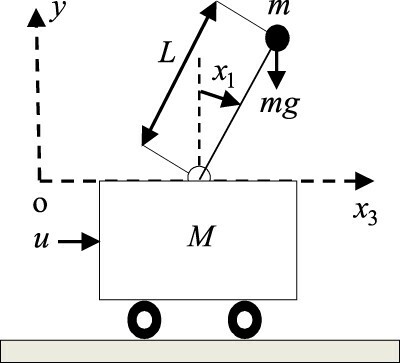
Consider the underactuated CIP system depicted in Figure 1. This system is described by the model [5]: (1) $\underset{\dot{x}}{\underbrace{\left[\begin{array}{c}{\dot{x}}_1\\ {\dot{x}}_2\\ {\dot{x}}_3\\ {\dot{x}}_4\end{array}\right]}}=\underset{f}{\underbrace{\left[\begin{array}{c}{x}_2\\ +f_1{x}_1\\ x_4\\ -f_2{x}_1\end{array}\right]}}+\underset{h}{\underbrace{\left[\begin{array}{c}0\\ -h_1\\ 0\\ +h_2\end{array}\right]}}u$(1) with the cart control input force $u(t)$ and the nonlinear functions $f_1$, $f_2$, $h_1$, and $h_2$ defined hereafter (2) $\begin{array}{l}{f}_1={\displaystyle \frac{(M+m)g{L}^{-1}-m{x}_2^2\cos x_1}{M+m-m{\cos }^2{x}_1}}{\displaystyle \frac{\sin x_1}{x_1}};\\ h_1={\displaystyle \frac{L^{-1}\cos x_1}{M+m-m{\cos }^2{x}_1}}\\ f_2={\displaystyle \frac{mg\cos x_1-mL{x}_2^2}{M+m-m{\cos }^2{x}_1}}{\displaystyle \frac{\sin x_1}{x_1}};\\ h_2={\displaystyle \frac{1}{M+m-m{\cos }^2{x}_1}}\end{array}$(2) where $g$ is the gravity acceleration, $x_1$ is the angular position of the pendulum with the origin at the upright position, $x_2$ is the pendulum angular velocity, $x_3$ and $x_4$ are the cart position and velocity. The inverted pendulum is characterized by a mass-less pole of length $L$ and a ball of mass $m$. The cart has a mass $M$ and moves under the action of $u(t)$ left or right on a one-dimensional horizontal bounded track.

Figure 1. The inverted pendulum system.

The following assumptions are considered:

Assumption 2.1:

The nonlinear functions $f_1$, $f_2$, $h_1$, and $h_2$ satisfy the bounded conditions: (3) $\begin{array}{rl}& \begin{array}{l}0<f_1<a_1;0<f_2<a_2\\ 0<h_1<b_1;0<h_2<b_2\end{array}\end{array}$(3) (4) $\begin{array}{rl}& \begin{array}{l}{x}_2^2+x_4^2+(a_1-f_1{)}^2+(a_2-f_2{)}^2<{\gamma }_f^2\\ (b_1-h_1{)}^2+(b_2-h_2{)}^2<{\gamma }_h^2\end{array}\end{array}$(4) where $a_1$, $a_2$, $b_1$, $b_2$, ${\gamma }_f$, and ${\gamma }_h$ are known positive numbers.

In system equations (1), we consider a space domain $D\subset R^4$ in which the $x_1$, $x_2$ and $x_4$ variable’ domains are implicitly defined using the bounded conditions (3) and (4) while the $x_3$variable’ domain is explicitly defined using $|x_3|<w_3$, where $2w_3$ is the track length. From (3), it is observed that $h_1>0$ implies that $|x_1|<\pi /2$ while $f_2>0$implies $f_1>0$ and $|x_2|<\sqrt{g{L}^{-1}\cos x_1}$. With an appropriate choice of $a_1$, $a_2$, $b_1$, $b_2$, ${\gamma }_f$, and ${\gamma }_h$, the bounded conditions in (3) and (4) consider the pendulum in the neighbourhood of its top unstable equilibrium position and specify the considered range of nonlinear model uncertainties.

Assumption 2.2:

The CIP physical parameters $M$, $m$ and $L$ are known from direct measurements.

In Assumption 2, we have considered that the CIP physical parameters are known to allow the problem of conversion to be solved easily without considering parameter uncertainties. Even if this assumption appears unreasonable to some extent, it is used in some recent papers, including [2] and [6] that are used in section 4. In addition to that experimental results conducted in [2] shows to support such a hypothesis to some extent for an SFC. On the other hand, Theorem 2.1 stated below shows some potential to take the CIP parameter uncertainties into account through the bounded conditions (4) but till now it is not clear to us how to conduct the trivial conversion in such a situation, so this issue is not yet undertaken in the present paper.

Assumption 2.3:

Small-angle approximations, i.e. $\sin x_1\approx x_1$ and $\cos x_1\approx 1$, and the small-angle velocity approximation, i.e. $x_2^2<<g{L}^{-1}$ are considered.

Assumptions 2 and 3 are used to derive the following approximate CIP linear model: (5) $\begin{array}{rl}\underset{\dot{x}}{\underbrace{\left[\begin{array}{c}{\dot{x}}_1\\ {\dot{x}}_2\\ {\dot{x}}_3\\ {\dot{x}}_4\end{array}\right]}}& =\underset{A}{\underbrace{\left[\begin{array}{cccc}0& 1& 0& 0\\ +a_1& 0& 0& 0\\ 0& 0& 0& 1\\ -a_2& 0& 0& 0\end{array}\right]}}\\ & \times \underset{x}{\underbrace{\left[\begin{array}{c}{x}_1\\ x_2\\ x_3\\ x_4\end{array}\right]}}+\underset{B}{\underbrace{\left[\begin{array}{c}0\\ -b_1\\ 0\\ +b_2\end{array}\right]}}u\end{array}$(5) with the upper bounds of the nonlinear functions in (3), i.e. $a_1$, $a_2$, $b_1$, and $b_2$, defined hereafter: (6) $\begin{array}{rl}{a}_1& =\left(1+\frac{m}{M}\right)g{L}^{-1};a_2=\frac{m}{M}g;\\ b_1& =\frac{1}{LM};b_2=\frac{1}{M}\end{array}$(6)

Assumption 2.4:

Suppose that $A-B{K}_0$ is asymptotically stable for a gain vector $K_0$.

Assumption 2.5:

Suppose that ${\gamma }_h<1$ and ${\alpha }_f<{\lambda }_{min}(Q)/{\lambda }_{max}(P)$ where $P=P^T>0$ is the solution of the Lyapunov matrix equation $(A-B{K}_0{)}^{T}P+P(A-B{K}_0)=-2Q$ for some $Q=Q^T>0$.

The existence of a class of linear state-feedback controllers that can stabilize the nonlinear model (1) in a portion of the domain $D$ is crucial. Otherwise, there is no meaning that can be attributed to the conversion process from a state-feedback to an output-feedback controller. Assumption 2.4 considers the linearized model (5) controllable and it is effectively the case since $det\left(\left[\begin{array}{cccc}B& AB& A^{2}B& A^{3}B\end{array}\right]\right)\ne 0$. Therefore, there exist linear state-feedback control laws with appropriate gain vectors that can successfully stabilize the system (1) to its unstable equilibrium position. Assumption 2.5 states supplementary conditions concerning the approximate region of attraction where the considered controller can effectively achieve the stabilization task. The justification for using linear state-feedback controllers to stabilize the nonlinear system (1) is stated in the following theorem, which is a simple adaptation of Theorem 4.4 in [24].

Theorem 2.1:

Under Assumptions 2.4 and 2.5, and the constraint $\gamma >0$, the linear state-feedback $u=-(K_0+\gamma B^{T}P)x$ stabilizes the nonlinear system (1) for arbitrary nonlinear functions $f_1$, $f_2$, $h_1$, and $h_2$ that satisfy the norm bounds (4).

Proof:

The proof of theorem 2.1 is quite similar to that presented for Theorem 4.4 in [24], and it is based on the Lyapunov method.

Assumption 2.6:

Absence of (accurate) velocity measurements.

Assumption 2.7:

The pendulum angle is contaminated by an additive high-frequency band noise $e_1$ while the cart position is measured without any errors (or at least the errors are so small so that they can be neglected).

The nonlinear model (1) is completed by the measured outputs: (7) $\begin{array}{l}{x}_{1m}=x_1+e_1\\ x_{3m}=x_3\end{array}$(7) For the CIP system stabilization, the goal is to drive the cart as quickly as possible from an initial position $x_3(0)$ to a constant final destination $x_{3d}$ without significant overshoot, undershoot, and control input effort while keeping the pendulum erected in the upright position, during such movement. To achieve this task, Theorem 2.1 states that under full-state availability, one possible solution is to use a linear SFC with an appropriate gain vector $N=(N_1,N_2,N_3,N_4)$. In this case, the control law of the SFC, which is mathematically equivalent to a TPD, takes the form: (8) $\begin{array}{rl}lu(t)& =-Nx(t)+N_3{x}_{3d}\\ & =-N_1{x}_1(t)-N_2{x}_2(t)-N_3[x_3(t)-x_{3d}]\\ & -N_4{x}_4(t)\end{array}$(8) where $x=(x_1,x_2,x_3,x_4{)}^T$ is the state variable vector.

The SFC gains of (8) can be adjusted to ensure several interesting steady and transient response behaviour for the CIP control system around the unstable equilibrium point [2–6]. However, there are several practical issues to deal with to make it more efficient. The first one is the high control input demand that appears at the beginning of the stabilization, i.e. $u(0)=-N_3[x_3(0)-x_{3d}]$, which is proportional to the distance between the cart's initial position and its destination. The second one emerges with the absence of (accurate) velocity measurements (Assumption 2.6). The third one results from the high sensitivity of the state-feedback control input to the pendulum angle sensor noise (see Equations (7) and (8) and Assumption 2.7). The last one is related to the tuning parameter problem that must be solved to meet the stabilization requirements. Given the importance of SFC in the CIP stabilization (see Theorem 2.1) and the importance of the observer-free OFC in overcoming their drawbacks, it appears interesting to investigate the feedback design as an output regulation problem with a class of controllers that has some relation with the SFC. To apply such an idea, we may thus formulate the feedback controller design in two successive steps as follows.

In the first step, we consider the following class of (error) output-feedback controllers: (9) $\begin{array}{l}u=\left[\begin{array}{cc}1& 0\end{array}\right]z\\ \dot{z}=H_{1}z+H_2{\left[\begin{array}{cc}0-x_{1m}& x_{3d}-x_{3m}\end{array}\right]}^T\\ z(0)={\left[\begin{array}{cc}0& 0\end{array}\right]}^T\end{array}$(9) where $z$is a state vector and $H_1$ with $H_2$ are two constant matrices. Under the above-mentioned assumptions, design a control law of the form (9), or equivalently find $z$, $H_1$ and $H_2$, such that the following properties are satisfied:

Property 2.1:

The control law (9) must be interpreted as a conversion of the state-feedback control law (8).

Property 2.2:

The equilibrium point of the closed-loop nonlinear CIP system must be asymptotically stable, or equivalently, the closed-loop linearized CIP system is stable.

Remark 2.1:

Property 1 allows converting any SFC to an OFC of the form (9). With such a conversion, the first three above-mentioned SFC drawbacks can be efficiently addressed. Indeed, the controller in (9) receives only the errors in the pendulum angle and cart positions that are filtered from the noise before reaching its output. In addition, the force applied at the beginning of stabilization is now null due to the zero initial conditions used in the controller state variables.

In the second step, the goal is to set the parameters $\phi$ of the proposed OFC to ensure a set of possible transient response requirements like fast cart response (reduced cart settling time), good stability (reduced cart overshoot, cart undershoot, and pendulum overshoot), and minimum control effort (reduced maximum control input effort). To solve such a problem, two issues must be addressed. The first one concerns the criterion choice while the second one concerns the adopted method to optimize it. Although there are several commonly used objective functions, we have found it useful from the comparison and the optimization point of view to build our own objective function $J(\phi )$ as the minimum between two new sound performance indices. These indices are the speed efficiency $S_E(\phi )$ and the average peak efficiency $S_E(\phi )$, and are defined for a given standard (reference) state-feedback method (SSF) and a given control method (CM), as follows: (10) $\begin{array}{rl}{S}_E(\phi )& =100\frac{P_{4,SSF}}{P_{4,CM}+P_{4,SSF}}\\ G_E(\phi )& =\frac{100}{3}\sum _{i=1}^3\frac{P_{i,SSF}}{P_{i,CM}+P_{i,SSF}}\end{array}$(10) where $P_{1,CM}$ is the maximum absolute value $P_{x1}$ of the pendulum angle response, $P_{2,CM}$ is the maximum absolute value between the overshoot $V_{x3}$ and undershoot $D_{x3}$ of the cart position response, $P_{3,CM}$ is the maximum absolute value $P_u$ of the control input signal, and $P_{4,CM}$ is the cart settling time $t_{cs}$ at 5%. The index $P_{i,SSF}$ has the same interpretation as the index $P_{i,CM}$, with the control method CM replaced by SSF.

The adopted definitions of speed and peak efficiencies allow not only concrete control method comparison but also help in building simple and efficient criteria for parameter tuning. Indeed, using such definitions, one can directly interpret the control method performance and indicate clearly if a method outperforms another one or not. For example, method CM outperforms completely the reference method SSF if both efficiencies are greater than 50%. The method CM is bad compared to SSF if both efficiencies are lower than 50%. In the remaining two cases, it is possible to identify the advantage the drawback of the CM over the SSF in terms of speed and peak efficiencies. With such an interpretation, we may formulate the CM setting problem as a maximin optimization model as follows: (11) $\begin{array}{rl}{\phi }_{opt}& =\underset{\phi }{\arg }\underset{\phi }{max}J(\phi )\\ J(\phi )& =min(S_E(\phi ),G_E(\phi ))\end{array}$(11) It should be noted that (11) is a continuous nonlinear optimization model with a highly nonlinear (possibly discontinuous) objective function $J(\phi )$ and it is difficult to know a priori whether such a function is unimodal or multimodal before starting the optimization. To avoid erroneous solutions, problem (11) has to be solved to global optimality in the considered parameter space domain. However, the direct search over all the stabilizing controllers is cumbersome, and, given the complexity of the objective function, there is no guarantee to obtain the optimal solution with standard global search techniques, especially when the number of tuning parameters is large. To reduce the challenge of this problem, we look for reducing the space search to develop a simple tuning method that gives suboptimal guarantee solutions but can be successfully applied to parameter tuning of other types of CIP system controllers, especially the TPD, the TPID, and the proposed OFC.

3. Controller design

To solve the above problems, we proceed constructively and simply. In the first step, we propose a modified version of the given SFC based on an appropriate cart change variable, which is initially proposed in [3]. Then, we convert the obtained modified SFC to an OFC and determine the conditions under which the final obtained linearized closed-loop system is stabilized. The conversion needs the development of a standard controller (state-feedback, state estimator, and internal model) as an intermediate step. In the second step, we propose two efficient methods to solve the parameter tuning problem.

3.1. Modified state-feedback controller

To make the analysis and processing of the approximate linear model (5) more general, let us reveal the link that exists between the parameters $a_1$ and $a_2$ as follows: (12) $\begin{array}{rl}{a}_2& ={\alpha }_1{a}_1-{\beta }_1;{\alpha }_1=\frac{b_2}{b_1}=L;\\ {\beta }_1& =\frac{a_1{b}_2-a_2{b}_1}{b_1}=g\end{array}$(12) where ${\alpha }_1$ and ${\beta }_1$ are two well-known positive parameters. Now, let us define the following change of variables [3] (13) $\begin{array}{rl}{y}_3& =x_3+{\alpha }_1{x}_1\\ y_4& =x_4+{\alpha }_1{x}_2\end{array}$(13)

Combining (5), (12), and (13), we obtain the following simplified linear model: (14) $\begin{array}{l}{\dot{x}}_1=x_2\\ {\dot{x}}_2=+a_1{x}_1-b_{1}u\\ {\dot{y}}_3=y_4\\ {\dot{y}}_4={\beta }_1{x}_1\end{array}$(14)

The above model has only three parameters that are summarized for convenience as follows: (15) $\begin{array}{rl}{a}_1& =\left(1+\frac{m}{M}\right)g{L}^{-1};b_1=\frac{1}{LM};{\beta }_1=g\end{array}$(15)

Applying the Laplace transform to (14) yields a modified open-loop CIP system composed of two sub-systems $H_1(s)$ and $H_3(s)$ in cascade. These sub-systems are unstable and are characterized by the transfer functions: (16) $\begin{array}{rl}{H}_1(s)& =\frac{X_1(s)}{U(s)}=\frac{-b_1}{s^2-a_1}\end{array}$(16) (17) $\begin{array}{rl}{H}_3(s)& =\frac{Y_3(s)}{X_1(s)}=\frac{{\beta }_1}{s^2}\end{array}$(17)

At this stage we modify slightly (8) to get the following new state-feedback control law: (18) $\begin{array}{rl}u(t)& =-N_1{x}_1(t)-N_2{x}_2(t)-N_3[y_3(t)-x_{3d}]\\ & -N_4{y}_4(t)\end{array}$(18)

Combining the Laplace transform of (18) with (16) and (17) yields the following closed-loop transfer functions: (19) $\begin{array}{rl}{F}_{1MSF}(s)& =\frac{X_1(s)}{X_{3d}(s)}\\ & =\frac{-b_1{N}_3{s}^2}{\begin{array}{c}{s}^4-b_1{N}_2{s}^3-(b_1{N}_1+a_1)s^2\\ -{\beta }_1{b}_1{N}_{4}s-{\beta }_1{b}_1{N}_3\end{array}}\\ F_{3MSF}(s)& =\frac{Y_3(s)}{X_{3d}(s)}\\ & =\frac{-{\beta }_1{b}_1{N}_3}{\begin{array}{c}{s}^4-b_1{N}_2{s}^3-(b_1{N}_1+a_1)s^2\\ -{\beta }_1{b}_1{N}_{4}s-{\beta }_1{b}_1{N}_3\end{array}}\end{array}$(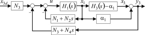19) The obtained closed-loop linearized CIP system is of the fourth order and has the basic configuration shown in Figure 2, where the real cart position $x_3$ is substituted by the modified position $y_3$. Notice that according to the necessary condition of stability of the system (19), the SFC gains $N=(N_1,N_2,N_3,N_4)$ must be real and negative.

Figure 2. Configuration of the modified state-feedback control.

Remark 3.1

Regarding the transformation (13), the modified control law (18) can be viewed as a conventional state-feedback law (8), in which the gain vector $N=(N_1,N_2,N_3,N_4)$ is substituted with $N_{new}=(N_1+{\alpha }_1{N}_3,N_2+{\alpha }_1{N}_4,N_3,N_4)$. This means that the first two gains are increased by the amounts ${\alpha }_1{N}_3$ and ${\alpha }_1{N}_4$, respectively. The well-known zeros of the cart transfer function (see Eq. B.1 in appendix B) associated with the original cart position variable $x_3$ are cancelled when using the new cart position variable $y_3$, as indicated in (19). As shown in the next section, the control law modification contributes to making the conversion from the SFC to an OFC a feasible task.

3.2. Proposed output-feedback controller

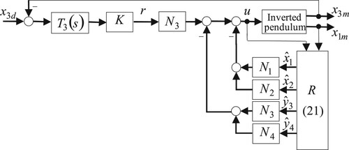
Now, we assume that the pendulum and the cart velocities are not measurable and that the pendulum angle is measured with noise as indicated by (7). An OFC can be obtained by combining the modified SFC (18), with an internal model $T_3(s)$ and a state estimator $R$, as shown in Figure 3. The parts of the proposed servo system are described in the following.

Figure 3. CIP servo system with internal model and state estimator.

To improve tracking for the step reference input $x_{3d}$ an internal model $T_3(s)$, in the form of a simple integrator, is employed in the control system. This integrator is associated with a positive gain $K$. The new reference input $r$ resulting from such internal model incorporation satisfies: (20) $\dot{r}=K(x_{3d}-x_{3m})$(20) In view of the approximate linear model (14), a reasonable proposed structure for the state estimator $R$ is given by the following open-loop state estimator: (21) $\begin{array}{l}{\dot{\hat{x}}}_1={\hat{x}}_2\\ {\dot{\hat{x}}}_2=a_1{x}_{1m}-b_{1}u\\ {\dot{\hat{y}}}_3={\hat{y}}_4\\ {\dot{\hat{y}}}_4={\beta }_1{x}_{1m}\end{array}$(21) where $({\hat{x}}_1,{\hat{x}}_2,{\hat{y}}_3,{\hat{y}}_4{)}^T$ is the state estimate of $(x_1,x_2,y_3,y_4{)}^T$. The state estimator (21) introduces in (14) one modification, which consists in substituting on the right-hand side of (14) the unmeasured state $x_1$ by the noisy measured signal $x_{1m}$.

Now, let us introduce the state vector $z={\left[\begin{array}{cc}{z}_1& z_2\end{array}\right]}^T$ with: (22) $\begin{array}{r}\begin{array}{l}{z}_1=u\\ z_2=N_1{\hat{x}}_2(t)+N_3{\hat{y}}_4\end{array}\end{array}$(22)

According to Figure 3, the control signal is given by: (23) $\begin{array}{rl}u& =z_1=-N_1{\hat{x}}_1(t)-N_2{\hat{x}}_2(t)\\ & -N_3{\hat{y}}_3(t)-N_4{\hat{y}}_4(t)+N_{3}r\end{array}$(23)

Taking the time-derivative of (23) and combining it with (20), (21) and (22) yields the control law (9) with: (24) $H_1=\left[\begin{array}{cc}-K_1& -1\\ +K_2& 0\end{array}\right],H_2=\left[\begin{array}{cc}-K_3& +K_5\\ +K_4& 0\end{array}\right]$(24) where the parameters of the above matrices are defined by the following simple canonical conversion: (25) $\begin{array}{l}{K}_1=-b_1{N}_2;K_2=-b_1{N}_1\\ K_3=a_1{N}_2+{\beta }_1{N}_4;K_4=a_1{N}_1+{\beta }_1{N}_3\\ K_5=K{N}_3\end{array}$(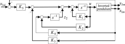25) Notice that $K_1$ and $K_2$ are real and positive while $K_3$, $K_4$ and $K_5$ are real and negative. The obtained CIP closed-loop system has the basic configuration shown in Figure 4, where the proposed OFC is defined by (9), (24), and (25).

Figure 4. Configuration of the proposed output-feedback-based CIP servo system.

With the transformation (25), Property 1 is satisfied and it remains to fulfil the local stability in Property 2. To this end, let us evaluate the closed-loop linearized CIP system transfer functions. In the noiseless situation, combining (16), (17) and (24) with the Laplace transform of (9) gives the following closed-loop transfer functions: (26) $\begin{array}{r}\begin{array}{rl}{F}_{1OF}(s)& =\frac{X_1(s)}{X_{3d}(s)}=\frac{-b_1{K}_5{s}^2}{\begin{array}{c}{s}^5+K_1{s}^4+(K_2-a_1)s^3\\ -(b_1{K}_3+a_1{K}_1-{\alpha }_1{b}_1{K}_5)s^2\\ -(b_1{K}_4+a_1{K}_2)s-{\beta }_1{b}_1{K}_5\end{array}}\\ F_{3OF}(s)& =\frac{Y_3(s)}{X_{3d}(s)}=\frac{-{\beta }_1{b}_1{K}_5}{\begin{array}{c}{s}^5+K_1{s}^4+(K_2-a_1)s^3\\ -(b_1{K}_3+a_1{K}_1-{\alpha }_1{b}_1{K}_5)s^2\\ -(b_1{K}_4+a_1{K}_2)s-{\beta }_1{b}_1{K}_5\end{array}}\end{array}\end{array}$(26) Assuming that the gains $N_i$, $1\le i\le 4$, of the state-feedback controller are known, it is possible to evaluate directly four of the five parameters of the proposed OFC via the transformation (25). In this situation, there is only a single tuning parameter $K$, or equivalently $K_5$, that is adjusted to ensure the stability of the systems $F_{1OF}(s)$ and $F_{3OF}(s)$, i.e Property 2. The stability conditions are given in the following theorem.

Theorem 3.2:

Suppose that the state-feedback controller gains $N_i$, $1\le i\le 4$, are negative. Under the assumption $\mathrm{\Delta }=(K_2-a_1{)}^2+4(b_1{K}_4+a_1{K}_2)>0$, the closed-loop systems defined by (26) are stable if the next condition holds (27) $\begin{array}{l}{K}_{min}<K<K_{max}\\ K_{min}=N_3^{-1}\underset{{\omega }^2\in \{0,{\omega }_2^2\}}{min}R({\omega }^2)\\ K_{max}=N_3^{-1}R({\omega }_1^2)\end{array}$(27) with (28) $\begin{array}{rl}R({\omega }^2)& =\frac{K_1{\omega }^2+a_1{K}_1+b_1{K}_3}{{\alpha }_1{b}_1{\omega }^2+{\beta }_1{b}_1}{\omega }^2\\ {\omega }_1^2& =0.5(K_2-a_1)\\ & -0.5\sqrt{{(K_2-a_1)}^2+4(b_1{K}_4+a_1{K}_2)}\\ {\omega }_2^2& =0.5(K_2-a_1)\\ & +0.5\sqrt{{(K_2-a_1)}^2+4(b_1{K}_4+a_1{K}_2)}\end{array}$(28)

Proof:

This theorem results directly from the application of the signature formulas to (26). The complete proof is given in Appendix A.

Remark 3.3:

For the stability analysis of the fifth-order closed-loop systems (26), in contrast to the signature formulas, the classical Routh criterion leads to an intricate set of highly nonlinear conditions that are difficult to exploit.

To perform well, the control system should at least be able to reject the effect of the measurement noise. Such effect on the control input can be described by using the Laplace transform of (9), which yields: (29) $\begin{array}{rl}U(s)& =C_{1OF}(s)(0-X_{1m}(s))\\ & +C_{3OF}(s)(X_{3d}(s)-X_{3m}(s))\end{array}$(29) (30) $\begin{array}{r}\begin{array}{rl}{C}_{1OF}(s)& =\frac{K_{3}s+K_4}{s^2+K_{1}s+K_2}\\ C_{3OF}(s)& =\frac{K_{5}s}{s^2+K_{1}s+K_2}\end{array}\end{array}$(30) The measurement noise $e_1(t)$ is injected into the control input through the filter $C_{1OF}(s)$. This filter exhibits a roll-off of high-frequency measurement noise with a slope of −20 dB per decade. The roll-off begins at the peak frequency: (31) $f_P=\frac{1}{2\pi }\sqrt{\begin{array}{c}-{\left(\frac{K_4}{K_3}\right)}^2\\ +\sqrt{{\left({\left(\frac{K_4}{K_3}\right)}^2+K_2\right)}^2-K_1^2{\left(\frac{K_4}{K_3}\right)}^2}\end{array}}$(31) Usually, the measurement noise $e_1(t)$ is of a high frequency; and if its bandwidth is located well above $f_P$, the filter will be effective in reducing this noise.

Remark 3.4:

In the development of the proposed OFC, we have considered that the CIP physical parameters are known (Assumption 2.2) to allow the problem of conversion to be solved easily without considering parameter uncertainties. When the parameter uncertainties are of major concern, the proposed method is still able to define a control scheme with five parameters (see Figure 4) that can be used to tackle directly the stabilization problem. In such a situation, the major concern may be how to tune the control scheme parameters without using the exact knowledge of the physical CIP parameters. Therefore, robust or adaptive controllers may be envisaged to solve such an issue.

Remark 3.5:

In the development of the proposed OFC, we have considered the open-loop state estimator (21) instead of a closed-loop state estimator. This rise some questions about its usefulness. Indeed, the cart integral controller and this estimator are only a tool to develop the OFC architecture without the addition of excessive tuning parameters. The estimator is not intended to achieve some perfect state estimations like the high-gain observers. However, regarding the fact that all the adjusted parts (internal model and state-feedback controller) and non-adjustable parts (state estimator and CIP system) in Figure 3 contribute together to give the control CIP system a final overall performance, the good parameter tuning of the adjusted parts will try to compensate to some extent the deficiencies of the proposed open-loop state estimator. This is addressed in the next sections.

3.3. Partial and global parameter tuning methods

To specify the gains of the proposed OFC there are two main approaches. The first one relies on the use of the transformation (25) and assumes that the gains $N$ of the SFC are given. In this case, we have a single parameter to tune $\phi =K$ to maximize the objective function $J(\phi )$ that appears in the optimization model (11). This method is referred to as the partial parameter tuning method.

The alternative global parameter tuning method aims in adjusting simultaneously all the five output-feedback controller parameters. In such a situation, we have $\phi =(K_1,K_2,K_3,K_4,K_5)$ or $\phi =(N_1,N_2,N_3,N_4,K)$ according to (25). To reduce the complexity of the above tuning problem while guaranteeing the optimality of the obtained solution, i.e avoid the repeatability problem associated with the use of optimization search methods [7], we shall only consider a coincident real negative pole configuration for all the obtained linearized control CIP systems. The coincident pole is denoted by $p$. With such a constraint, the controller gains can be analytically expressed with one single parameter $\phi =p$, which renders the tuning parameter an easy task. Applying this pole placement design directly on the closed-loop transfer functions (26) yields the following analytical gains for the proposed OFC: (32) $\begin{array}{rl}{K}_1& =-5p\\ K_2& =10p^2+a_1\\ K_3& ={\alpha }_1{{\beta }_1}^{-1}{b}_1^{-1}{p}^5+10b_1^{-1}{p}^3+5b_1^{-1}{a}_{1}p\\ K_4& =-5b_1^{-1}{p}^4-10b_1^{-1}{a}_1{p}^2-b_1^{-1}{a}_1^2\\ K_5& ={{\beta }_1}^{-1}{b}_1^{-1}{p}^5\end{array}$(32) Since the gains (32) of the OFC depend only on the chosen real negative pole $p$, solving the optimization problem (11) that tries to maximize $J(\phi )=J(p)$ with standard optimization technique becomes an easy task. Also, from the optimality point of view, it is clear that the global parameter tuning method (32) outperforms is in most cases the partial parameter tuning method.

4. Numerical simulations

Consider the nonlinear CIP system (1) and (2) with a set of physical parameters $M=2.4\text{kg}$, $m=0.23\text{kg}$, $L=0.36\text{m}$, $g=9.81\text{m/}{\text{s}}^{\text{2}}$, and a cart track length limited between $\pm 0.5\text{m}$ [5]. Numerical simulations are conducted in two separate sections to show the advantage of the proposed OFC with the partial and global tuning methods. In both sections, we adopt the SFC of [2] as a reference control method and symbolize it by SSF. The first main reason for this reference choice is linked to its best performance, as is claimed by its authors, especially in terms of speed efficiency. The second main reason is related to the fact that the gains of such a method are described analytically and there is no free parameter to tune, as is indicated hereafter for the considered CIP model: (33) $\begin{array}{l}{N}_{1SSF}=-3Mg;N_{2SSF}=-3Mg{z}^{-1}\\ N_{3SSF}=-0.2M{z}^2;N_{4SSF}=-1.2Mz\end{array}$(33) where $z=\sqrt{g{L}^{-1}}$.

In the first section, we are interested in using the partial parameter tuning method to design the proposed OFC. To this end, we shall study the impact of the proposed conversion (25) on the performances of the TPD and LQR state-feedback methods, which are presented in [5] for the same CIP system, and on the performances of the SSF method. Notice that the choice of the gains for the TPD and LQR methods are done in [5] using a trial and error method while the analytical gains (33) of the SSF method are derived from the optimization of a convenient criterion [2]. The parameters of the above-cited state-feedback controllers are listed in Table 1. The goal of this section is to highlight the potential applicability of our conversion method (25) with a rudimentary partial parameter tuning method and the need to modify the initial SFC if the controlled CIP system shows limited performance.

Table 1. Gains of the state-feedback controllers.

	$N_1$	$N_2$	$N_3$	$N_4$
SSF	$\phantom{1}-70.63$	$-13.53$	$-13.08$	$-15.03$
TPD	$\phantom{1}-40.00$	$\phantom{1}-8.00$	$\phantom{1}-1.00$	$\phantom{1}-3.00$
LQR	$-137.79$	$-25.98$	$-22.36$	$-27.58$

In the second section, we are interested in comparing the OFC, SFC, and TPID that are designed using the global tuning method within the context of coincident real pole configuration. This approach allows us to obtain rapidly a guaranteed optimality result for the tuned controller and avoid the repeatability problem that may occur when using advanced optimizing tuning methods [7] in conjunction with non constrained pole configuration. The structure of the TPID is chosen to allow output-feedback processing and to have exactly five tuning parameters as in the proposed OFC. The set of obtained TPID controllers that have these properties [6] are the PID-P and PI-PD controllers. Since the PI-PD with the coincident pole configuration shows very limited performance, we thus retain only the PID-P controller and refer to it hereafter as the PID controller. The derivation of the analytical expressions for the gains of the SFC and the considered PID controllers are given in Appendix B.

4.1. Partial tuning method design

To compare the performance of the SSF, LQR, and TPD controllers, the reference cart position $x_{3d}$ is set to$0\text{m}$, and all the initial state values are set to zeros except the initial cart position which is set to$x_3(0)=-0.1\text{m}$. The simulation results for the pendulum angle, cart position, and control input, without considering noise, are shown in Figures 5 and 6, and Table 2. Regarding the fact that we are concerned with a stabilization problem with null references, the cart position, the pendulum angle, and the control effort in Figures 5 and 6 become effectively error signals and the used performance indices ($P_{x1}$,$V_{x3}$,$D_{x3}$,$P_u$) can therefore naturally be interpreted as error indices. Now, it is observed that the TPD method exhibits the best $G_E$ of about $88\mathrm{\%}$, due to its relatively low peak values, at the price of a bad $S_E$ of $24\mathrm{\%}$. The LQR method exhibits a slightly better $G_E$ than the SSF method and has a nice and smooth cart response at the price of an increase in the control input effort and a slight degradation in $S_E$.

Figure 5. Pendulum angle and cart position responses using SSF, LQR, and TPD methods.

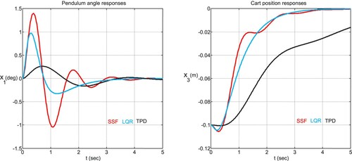
Figure 6. Control input responses using SSF, LQR, and TPD methods.

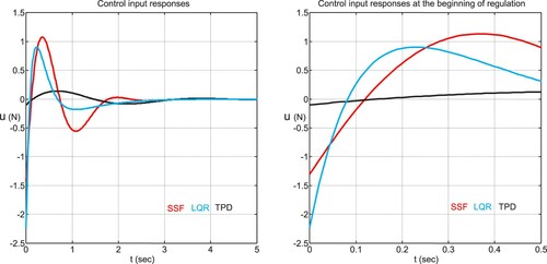
Table 2. Performance comparison of the control methods.

	$P_{x1}$ (deg)	$V_{x3}$ (%)	$D_{x3}$ (%)	$P_u(\text{N})$	$t_{cs}$ (sec)	$S_E$ (%)	$G_E$ (%)
SSF	$1.40$	$0.00$	$5.51$	$1.31$	$2.55$	$50.00$	$50.00$
SOF	$0.22$	$2.51$	$0.40$	$0.12$	$4.81$	$34.65$	$82.26$
TPD	$0.26$	$0.00$	$0.63$	$0.14$	$8.01$	$24.15$	$88.10$
MPD	$0.09$	$25.75\phantom{1}$	$0.07$	$0.04$	$19.37\phantom{1}$	$11.63$	$69.46$
LQR	$0.97$	$0.00$	$4.47$	$2.24$	$2.63$	$49.23$	$50.34$
MLQ	$0.17$	$3.85$	$0.31$	$0.09$	$4.57$	$35.81$	$80.59$

From the above-obtained results, it is clear that the state-feedback controllers are prone to high control effort demand that appears at the beginning of the pendulum regulation (Figure 6) and to cart transient response (undershoot) peaking phenomenon (Figure 5); and in the absence of velocity measurements, they cannot be applied directly to stabilize the CIP system. To overcome these difficulties the proposed OFC, defined by (9) and (25), is applied to all considered state-feedback controllers to get the output-feedback controllers SOF (standard output-feedback), MPD (modified TPD), and MLQ (modified LQR) associated to the state-feedback controllers SSF, TPD, and LQR, respectively. To apply our conversion technique, we need to tune the single parameter $K$ in such a way as to ensure closed-loop system stability and acceptable performance. To this end, a numerical investigation of stability conditions (27–28) for the above methods is performed and the obtained results are summarized in Table 3. A common zeros lower bounds $K_{min}=0$ and distinct uppers bounds are noticed.

Table 3. Lower and upper bounds of $K$ for SOF, MPD, and MLQ methods.

	$\text{SOF}$	$\text{MPD}$	$\text{MLQ}$
$K_{min}$	$0.00$	$0.00$	$0.00$
$K_{max}$	$2.27$	$1.70$	$1.85$

The effect of varying the parameter $K$ between $0.01$ and $1$ on $S_E$ and $G_E$ is shown in Figure 7. A clear decreasing trend for the average efficiency index $G_E$ with the increase of $K$ is observed for all considered CMs. The SOF and MLQ methods exhibit a similar $G_E$ trend. They perform better than the MPD method in the range $0.12<K<0.6$. Concerning the efficiency index $S_E$, an interesting increasing trend is observed for the low-value side of $K$. The value of $K$ at which this increasing trend stop is a CM dependent. The MPD method presents the shortest interval and the SOF present the largest one. The SOF and MLQ methods exhibit similar $S_E$ trend in the interval $0.01\le K\le 0.4$.

Figure 7. Effect of $K$ on the speed and average peak efficiencies for SOF, MLQ, and MPD methods.

As a general remark, it is noted that the introduction of our partial tuning-based conversion technique to the SSF and LQR methods leads to a substantial improvement of $G_E$ at the price of an eventual degradation of $S_E$. Among the studied CMs, the MPD method appears to be the worst one in term of $S_E$ and cannot achieve more than $18\mathrm{\%}$ (Figure 7). The SOF and MLQ methods show interesting $S_E$ performances; and if the parameter $K$ is appropriately adjusted, these methods can achieve the highest $S_E$ with a value of $37\mathrm{\%}$ at the price of a relatively slightly low value of $G_E$ of $76\mathrm{\%}$ (Figure 7). Compared with the state-feedback controllers, the proposed output-feedback controllers have always better $G_E$ performance and relatively low $S_E$ performance. This means that the state-feedback $S_E$ performance can only be recovered to some extent with the proposed partial tuning-based output-feedback conversion technique when it is applied to the considered state-feedback controllers. The improvement of the speed of response of the CIP can be obtained using the global parameter tuning as discussed below in the next section.

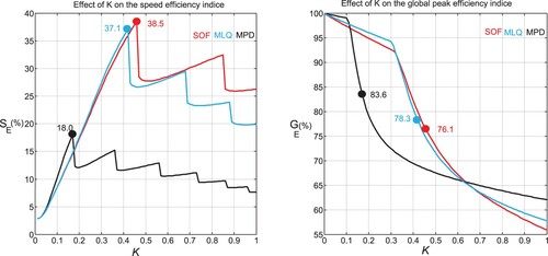
The simulation results with $K=0.4$ for the pendulum angle, cart position, and control input, without considering noise, for the studied partial tuning-based output-feedback controllers are shown in Figures 8 and 9 and Table 2. It is observed that the SOF and MLQ methods exhibit similar $S_E$ in the vicinity of $34.5\mathrm{\%}$, which is relatively large in comparison to $11.63\mathrm{\%}$ of the MPD method. The introduction of the proposed OFC on the original SFC leads on the first hand to the decrease of the pendulum angle overshoot, the cart undershoot, and the control input overshoot, and on the other hand to the increase of the cart position overshoot and the cart settling time.

Figure 8. Pendulum angle and cart position responses using SOF, MLQ, and MPD methods.

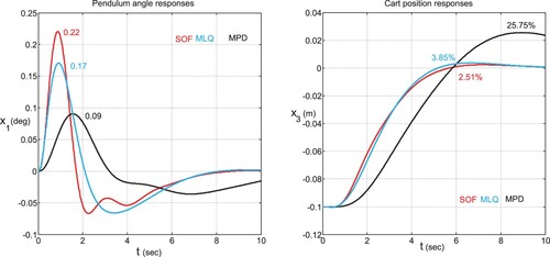
Figure 9. Control input responses using SOF, MLQ, and MPD methods.

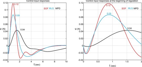
4.2. Global tuning method design

Table 4 shows the effect of the pole $p$ on the performance of the SFC, OFC, and PID controllers. It is observed that the increase of $p$ leads for the above controllers to a decrease in the pendulum angle overshoot, the cart position overshoot, the cart position undershoot, and in the control input effort in addition to an increase in the cart settling time. The OFC and PID controller show quite similar performance. The SFC outperforms the other controllers in the cart position overshoot and the cart settling time but shows less interesting behaviours in the remaining transient control CIP system response characteristics. The obtained optimal gains for the above three controllers are listed in Table 5, where it is observed that the gains associated with the proposed OFC controllers appear to be somewhat higher than the other controller gains. Figure 10 presents the effect of varying $p$ on the peak frequency $f_P$ of the filter $C_{1OF}(s)$ and on the efficiency performance index $J(p)=min(S_E,G_E)$ of the SFC and OFC controllers. The results associated with the PID method are not shown in Figure 10 since there are very close to those of the OFC method. For a given pole $p>-3.73$, the OCF can recover at least 92% of the SFC efficiency while for a given pole $p<-3.73$, the OCF becomes more efficient than the OSC method. The best efficiency record for the SFC is about 55% at $p=-3.55$ and the best efficiency record for the OFC is about 57.4% at $p=-4.59$. The OFC needs a somewhat higher bandwidth to recover the performance of the SFC as is indicated by the OFC peak frequency curve, which tends to increase with the decrease of the real negative pole $p$. The OFC peak frequency is $1.8\text{Hz}$ at $p=-3.55$ and $2.3\text{Hz}$ at $p=-4.59$.

Figure 10. Effect of $p$ on the peak frequency and on efficiency indices for SFC and OFC methods.

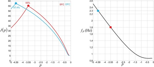
Table 4. Performance comparison of the SFC, OFC, and PID methods.

	$P_{x1}$ (deg)			$V_{x3}(\mathrm{\%})-D_{x3}(\mathrm{\%})$			$P_u$ (N)			$t_{CS}$ (sec)
$p$	$\text{SFC}$	$\text{OFC}$	$\text{PID}$	$\text{SFC}$	$\text{OFC}$	$\text{PID}$	$\text{SFC}$	$\text{OFC}$	$\text{PID}$	$\text{SFC}$	$\text{OFC}$	$\text{PID}$
$-1$	$0.08$	$0.05$	$0.05$	$0-0.09$	$0-0.02$	$0-0.03$	$0.04$	$0.02$	$0.03$	$7.71$	$9.12$	$8.90$
$-2$	$0.31$	$0.21$	$0.21$	$0-0.82$	$0-0.33$	$0-0.37$	$0.17$	$0.11$	$0.11$	$3.82$	$4.53$	$4.42$
$-3$	$0.69$	$0.47$	$0.48$	$0-2.57$	$0.02-1.24$	$0-1.35$	$0.71$	$0.28$	$0.29$	$2.51$	$2.98$	$2.91$
$-4$	$1.22$	$0.84$	$0.86$	$0-5.42$	$0.03-2.90$	$0.01-3.09$	$2.25$	$0.59$	$0.61$	$1.83$	$2.20$	$2.14$
$-5$	$1.91$	$1.32$	$1.34$	$0-9.35$	$0.07-5.34$	$0.02-5.62$	$5.50$	$1.11$	$1.15$	$1.42$	$1.71$	$1.67$

Table 5. Optimal gains for the SFC, OFC, and PID methods.

$\text{SFC}$	$N_1=-96.17$	$N_2=-17.94$	$N_3=-13.99$	$N_4=-15.76$
$\text{OFC}$	$K_1=22.95$	$K_2=240.54$	$K_3=-1492.2$	$K_4=-8123.6$	$K_5=-179.43$
$\text{PID}$	$K_{11}=-65.02$	$K_{12}=-80.21$	$K_{13}=-9.18$	$K_{31}=-7.82$	$T_1=0.0436$

To check the ability of the SSF controller and the optimal SFC, OFC, and PID controllers to reject noise, a uniform random noise $e_1(t)$ with the values restricted to the interval $|e_1(t)|<A$, with $A={10}^{-3}$, and sampling time $0.01\text{ sec}$ is added to the pendulum angle state over a time interval of $120\sec$. Table 6 summarizes the obtained maximum absolute value for the CIP input and outputs over the last $100\sec$ for each considered CM. It is observed that the SSF and optimal SFC methods tend to perform similarly. It is also observed that the optimal OFC outperforms the optimal PID in the performance of the control input while the optimal PID outperforms to some extent the optimal OFC in the performance of the CIP outputs. All the considered controllers give acceptable stabilization performance in the considered noisy situation. Figures 11–13 illustrate graphically the impact of noise on the performance of the control system input and outputs for the above-considered controllers. The carried simulation results show the effectiveness of the proposed OFC in comparison to the SSF and its competitiveness with the best five-parameter PID controllers.

Figure 11. Pendulum angle responses in a noisy situation.

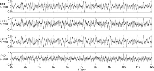
Figure 12. Cart position responses in a noisy situation.

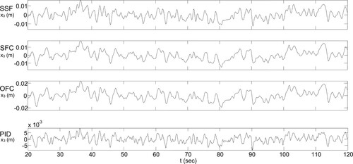
Figure 13. Control input responses in a noisy situation.

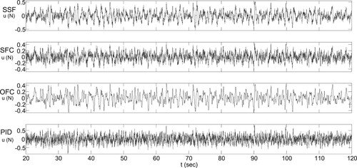
Table 6. Performance comparison in noisy situation.

	SSF	SFC	OFC	PID
$max(|x_1|)$ (deg)	$0.624$	$0.459$	$0.622$	$0.546$
$max(|x_3|)$ (m)	$0.016$	$0.018$	$0.023$	$0.008$
$max(|u|)$ (N)	$0.541$	$0.480$	$0.472$	$0.863$

5. Conclusion

Conventional CIP state-feedback controllers are prone to several difficulties. To deal with the high control effort demand that appears at the beginning of the pendulum regulation, the cart transient response peaking phenomenon, and implementation difficulties due to the absence of (accurate) velocity measurements, the given static state-feedback controller was converted to a second-order output-feedback controller by introducing a comprehensive transformation. Local system stability analysis is conducted using the signature formulas method to get simple conditions. The control scheme parameters were tuned using partial and global parameter tuning methods and compared with several well-known state and output-feedback controllers. Future work will be devoted to conducting a more rigorous stability analysis for the controlled nonlinear system; improving the performance of the developed output-feedback controller by optimizing its gains in the context of more efficient pole configurations; and relaxing certain assumptions used in the development of the proposed method. For taking the physical CIP parameter uncertainties into account, it may be interesting to exploit directly the obtained controller structure to build robust and/or adaptive controllers. It may be also useful to examine if the above-cited structure allows defining a more convenient sliding surface to reduce the impact of chattering when using a standard sliding mode controller to stabilize the CIP system. Finally, how to adapt the proposed method directly to the nonlinear CIP or other robotic systems without using a linearization step is also an interesting axis of research.

Disclosure statement

No potential conflict of interest was reported by the author(s).

Additional information

Funding

This work was supported by the Ministry of Higher Education and Scientific Research of Algeria (PRFU A01L08UN210120220001), by PHC Tassili project (project code: 43790QB) and by Slovenian Research Agency (ARRS) with the Research Program P2-0219.

Appendices

Appendix A: Proof of Theorem 3.2

The proof of Theorem 3.2 is conducted using the signature formulas method that is described in [23, p.40-53]. To this end, let us consider the characteristic polynomial of (26), which is without zeros on the imaginary axis and has a single tuning parameter. Then, write it in the following form: (A1) $\begin{array}{rl}\delta (s,K_5)& ={\delta }_{even}(s^2)+s{\delta }_{odd}(s^2)\\ {\delta }_{even}(s^2)& =K_1{s}^4-(b_1{K}_3+a_1{K}_1-{\alpha }_1{b}_1{K}_5)s^2-{\beta }_1{b}_1{K}_5\\ {\delta }_{odd}(s^2)& =s^4+(K_2-a_1)s^2-(b_1{K}_4+a_1{K}_2)\end{array}$(A1) so that (A2) $\begin{array}{rl}\delta (j\omega )& ={\delta }_r(\omega )+j{\delta }_i(\omega )\\ {\delta }_r(\omega )& ={\delta }_{even}(-{\omega }^2)=K_1{\omega }^4+(b_1{K}_3+a_1{K}_1\\ & -{\alpha }_1{b}_1{K}_5){\omega }^2-{\beta }_1{b}_1{K}_5\\ {\delta }_i(\omega )& =\omega {\delta }_{odd}(-{\omega }^2)=\omega [{\omega }^4-(K_2-a_1){\omega }^2\\ & -(b_1{K}_4+a_1{K}_2)]\end{array}$(A2)

It is clear from (A1) that only the even part of $\delta (s,K_5)$ depends on $K_5$. Under the following condition: (A3) $\mathrm{\Delta }=(K_2-a_1{)}^2+4(b_1{K}_4+a_1{K}_2)>0$(A3)

The real nonnegative zeros of ${\delta }_i(\omega )$ with odd multiplicities, i.e. ${\omega }_1$and ${\omega }_2$, with ${\omega }_0=0$ are given by: (A4) $\begin{array}{rl}{\omega }_0& =0\\ {\omega }_1^2& =\frac{K_2-a_1-\sqrt{{(K_2-a_1)}^2+4(b_1{K}_4+a_1{K}_2)}}{2}\\ {\omega }_2^2& =\frac{K_2-a_1+\sqrt{{(K_2-a_1)}^2+4(b_1{K}_4+a_1{K}_2)}}{2}\end{array}$(A4)

According to Lemma 2.1 and Theorem 2.1 of [23], the Hurwitz signature of the five-order polynomial $\delta (s,K_5)$ is given by: (A5) $\begin{array}{rl}\sigma (\delta )& =l-r=\mathrm{sgn}[{\delta }_i(0^{+}){]}^{}(\mathrm{sgn}[{\delta }_r(0)]-2\mathrm{sgn}[{\delta }_r({\omega }_1)]\\ & +2\mathrm{sgn}[{\delta }_r({\omega }_2)])\\ {\delta }_i(0^{+})& =0^{+}\\ {\delta }_r(0)& =-{\beta }_1{b}_1{K}_5\\ {\delta }_r({\omega }_1)& =K_1{\omega }_1^4+(b_1{K}_3+a_1{K}_1-{\alpha }_1{b}_1{K}_5){\omega }_1^2-{\beta }_1{b}_1{K}_5\\ {\delta }_r({\omega }_2)& =K_1{\omega }_2^4+(b_1{K}_3+a_1{K}_1-{\alpha }_1{b}_1{K}_5){\omega }_2^2-{\beta }_1{b}_1{K}_5\end{array}$(A5) where $l$ is the number of stable poles, $r$ is the number of unstable poles, and $\mathrm{sgn}[\cdot ]$ is the signum function that is defined as follows: (A6) $\mathrm{sgn}[x]=\{\begin{array}{ll}-1& \text{if }x<0\\ 0& \text{if }x=0\\ +1& \text{if }x>0\end{array}$(A6)

From (A5) it is obvious that for the five-order polynomial $\delta (s,K_5)$ to be Hurwitz, it is necessary and sufficient to have: (A7) $\begin{array}{rl}{\delta }_r(0)& =-{\beta }_1{b}_1{K}_5>0\\ {\delta }_r({\omega }_1)& =K_1{\omega }_1^4+(b_1{K}_3+a_1{K}_1-{\alpha }_1{b}_1{K}_5){\omega }_1^2\\ & -{\beta }_1{b}_1{K}_5<0\\ {\delta }_r({\omega }_2)& =K_1{\omega }_2^4+(b_1{K}_3+a_1{K}_1-{\alpha }_1{b}_1{K}_5){\omega }_2^2\\ & -{\beta }_1{b}_1{K}_5>0\end{array}$(A7)

After some obvious independent algebraic manipulations, the inequalities of (A7) can be further reduced to: (A8) $\begin{array}{l}{K}_5<0\\ K_5>{\displaystyle \frac{K_1{\omega }_1^4+(b_1{K}_3+a_1{K}_1){\omega }_1^2}{{\alpha }_1{b}_1{\omega }_1^2+{\beta }_1{b}_1}}\\ K_5<{\displaystyle \frac{K_1{\omega }_2^4+(b_1{K}_3+a_1{K}_1){\omega }_2^2}{{\alpha }_1{b}_1{\omega }_2^2+{\beta }_1{b}_1}}\end{array}$(A8)

From (A8) and $K_5=K{N}_3$ in eq (25), we get finally: (A9) $\begin{array}{l}{K}_{min}<K<K_{max}\\ K_{min}=N_3^{-1}\underset{{\omega }^2\in {\{0,{\omega }_2^2\}}^{}}{min}R({\omega }^2)\\ K_{max}=N_3^{-1}R({\omega }_1^2)\end{array}$(A9) with (A10) $R({\omega }^2)=\frac{K_1{\omega }^2+a_1{K}_1+b_1{K}_3}{{\alpha }_1{b}_1{\omega }^2+{\beta }_1{b}_1}{\omega }^2$(A10)

Appendix B: SFC and PID pole coincident-based gains

Let us first begin with the tuning of the SFC controller (8). Applying the Laplace transform to (5) and (8) yields the following closed-loop transfer functions: (B1) $\begin{array}{r}\begin{array}{rl}{F}_{1SF}(s)& =\frac{X_1(s)}{X_{3d}(s)}=\frac{-b_1{N}_3{s}^2}{\begin{array}{c}{s}^4-(b_1{N}_2-b_2{N}_4)s^3\\ -(b_1{N}_1-b_2{N}_3+a_1)s^2-b_1{N}_4{\beta }_{1}s\\ -b_1{N}_3{\beta }_1\end{array}}\\ F_{3SF}(s)& =\frac{X_3(s)}{X_{3d}(s)}=\frac{b_1{N}_3{\alpha }_1(s^2-{\alpha }_1^{-1}{\beta }_1)}{\begin{array}{c}{s}^4-(b_1{N}_2-b_2{N}_4)s^3\\ -(b_1{N}_1-b_2{N}_3+a_1)s^2-b_1{N}_4{\beta }_{1}s\\ -b_1{N}_3{\beta }_1\end{array}}\end{array}\end{array}$(B1)

For these sub-systems, the transfer function $F_{1SF}(s)$ has a fixed double zero at the origin and the transfer function $F_{3SF}(s)$ has two fixed zeros at $\pm \sqrt{{\alpha }_1^{-1}{\beta }_1}$. Thus, whatever the method used to specify the state-feedback controller gains, it is always interpreted as a kind of pole placement. In addition, the presence of a positive zero makes the CIP system a nonminimum phase. Now, taking into account the usefulness of driving the cart system with little or no oscillation (under and overshoot) to $x_{3d}$, we propose to specify the gains $(N_1,N_2,N_3,N_4)$ to obtain a coincident real negative pole $p$ structure for the targeted closed-loop system $F_{3SF}(s)$. In this situation, we get: (B2) $\begin{array}{r}\begin{array}{rl}{N}_1& =-{\alpha }_1{\beta }_1^{-1}{b}_1^{-1}{p}^4-6b_1^{-1}{p}^2-b_1^{-1}{a}_1\\ N_2& =+4{\alpha }_1{\beta }_1^{-1}{b}_1^{-1}{p}^3+4b_1^{-1}p\\ N_3& =-{\beta }^{-1}{b}_1^{-1}{p}^4\\ N_4& =+4{\beta }^{-1}{b}_1^{-1}{p}^3\end{array}\end{array}$(B2)

The structure of the output-feedback TPID controller can be defined by [6]: (B3) $\begin{array}{rl}U(s)& =C_{1PID}(s)(0-X_{1m}(s))+C_{3PID}(s)\\ & \times (X_{3d}(s)-X_{3m}(s))\end{array}$(B3) (B4) $\begin{array}{r}\begin{array}{rl}{C}_{1PID}(s)& =\frac{K_{13}{s}^2+K_{11}s+K_{12}}{s(1+T_{1}s)}\\ C_{3PID}(s)& =\frac{K_{33}{s}^2+K_{31}s+K_{32}}{s(1+T_{3}s)}\end{array}\end{array}$(B4) where $K_{1PID}=(K_{11},K_{12},K_{13},T_1)$ are the gains associated with the pendulum sub-system and $K_{3PID}=(K_{31},K_{32},K_{33},T_3)$ are the gains associated with the cart sub-system. There are 16 possible combinations of the TPID controllers that can be classified into unstable, redundant, underdetermined, and feasible setups [6]. The only feasible TPID controllers that have five parameters (The same number of parameters of the proposed OFC) are the PID-P and the PI-PD [6]. The filters associated with the considered PID-P (called PID in section 4) controllers are given by: (B5) $\begin{array}{r}\begin{array}{rl}{C}_{1PID}(s)& =\frac{K_{13}{s}^2+K_{11}s+K_{12}}{s(1+T_{1}s)}\\ C_{3P}(s)& =K_{31}\end{array}\end{array}$(B5)

Combining (B5), (40), and the Laplace transform of (11) gives the following five-order transfer functions: (B6) $\begin{array}{r}\begin{array}{rl}{F}_{1PID-P}(s)& =\frac{X_1(s)}{X_{3d}(s)}=\frac{A_{1PID-P}(s)}{D_{PID-P}(s)}\\ F_{3PID-P}(s)& =\frac{X_3(s)}{X_{3d}(s)}==\frac{A_{3PID-P}(s)}{D_{PID-P}(s)}\end{array}\end{array}$(B6) with (B7) $\begin{array}{r}\begin{array}{rl}{A}_{1PID-P}(s)& =-K_{31}{b}_1(s+T_1^{-1})s^2\\ A_{3PID-P}(s)& =K_{31}(b_2{s}^3+T_1^{-1}{b}_2{s}^2-b_1{\beta }_{1}s-T_1^{-1}{b}_1{\beta }_1)\\ D_{PID-P}(s)& =s^5+T_1^{-1}{s}^4-(a_1-b_2{K}_{31}+T_3^{-1}{b}_1{K}_{13})s^3\\ & -T_1^{-1}(a_1+b_1{K}_{11}-b_2{K}_{31})s^2\\ & -(T_1^{-1}{b}_1{K}_{12}+b_1{K}_{31}{\beta }_1)s-T_1^{-1}{b}_1{K}_{31}{\beta }_1\end{array}\end{array}$(B7)

The gains associated with the controllers (B5) taking the coincident real pole configuration into account for the closed-loop linearized CIP system is deduced from the denominator in (B6) as follows: (B8) $\begin{array}{r}\begin{array}{rl}{K}_{11}& =-(1/5){\alpha }_1{{\beta }_1}^{-1}{b}_1^{-1}{p}^4-2b_1^{-1}{p}^2-a_1{b}_1^{-1}\\ K_{12}& =(24/25)b_1^{-1}{p}^3\\ K_{13}& =\frac{b_2{p}^4+50b_1{\beta }_1{p}^2+5a_1{b}_1{\beta }_1}{25b_1^2{\beta }_{1}p}\\ K_{31}& =-(1/5){{\beta }_1}^{-1}{b}_1^{-1}{p}^4\\ T_1& =-(1/5)p^{-1}\end{array}\end{array}$(B8)

References

- Boubaker O. The inverted pendulum benchmark in nonlinear control theory: a survey. Int J Adv Rob Syst. 2013;10:1–9.
- Chatterjee S, Das SK. An analytical formula for optimal tuning of the state feedback controller gains for the cart-inverted pendulum system. IFAC-PapersOnLine. 2018;51(1):668–672.
- Messikh L, Guechi EH, Benloucif ML. Critically damped stabilization of inverted-pendulum systems using continuous-time cascade linear model predictive control. J Franklin Inst. 2017;354(16):7241–7265.
- Shehu M, Ahmad MR, Shehu A, et al. LQR, double-PID, and pole placement stabilization and tracking control of single link inverted pendulum. In 2015 IEEE International Conference on Control System, Computing and Engineering (ICCSCE) (pp. 218-223). IEEE; 2015, November.
- Prasad LB, Tyagi B, Gupta HO. Optimal control of nonlinear inverted pendulum system using PID controller and LQR: performance analysis without and with disturbance input. Int J Autom Comput. 2014;11(6):661–670.
- Kuczmann M. Comprehensive survey of PID controller design for the inverted pendulum. Acta Technica Jaurinensis. 2019;12:55–81.
- Önen Ü, Cakan A, Ilhan I. Performance comparison of optimization algorithms in LQR controller design for a nonlinear system. Turkish J Electr Eng Comput Sci. 2019;27(3):1938–1953.
- Saleem O, Rizwan M, Mahmood-ul-Hasan K. Self-tuning state-feedback control of a rotary pendulum system using adjustable degree-of-stability design. Automatika. 2021;62(1):84–97.
- Krishnan TR. On stabilization of cart-inverted pendulum system: An experimental study. Master thesis, Department of electrical engineering, National Institute of technology, India; 2012.
- Lee J, Mukherjee R, Khalil HK. Output feedback stabilization of inverted pendulum on a cart in the presence of uncertainties. Automatica (Oxf). 2015;54:146–157.
- Poloni T, Kolmanovsky I, Rohal’-Ilkiv B. Simple input disturbance observer-based control: case studies. J Dyn Syst Meas Contr. 2018;140:146–157.
- Katariya AS. (2010). Optimal state-feedback and output-feedback controllers for the wheeled inverted pendulum system. Thesis, School of electrical and computer engineering, Georgia institute of technology.
- Ovalle L, Ríos H, Llama M. Robust output-feedback control for the cart-pole system: a coupled super-twisting sliding-mode approach. IET Control Theory Applic. 2019;13(2):269–278.
- Aguilar-Ibáñez C, Suarez-Castanon MS, Cruz-Cortés N. Output feedback stabilization of the inverted pendulum system: a Lyapunov approach. Nonlinear Dyn. 2012;70:767–777.
- Isidori A, Byrnes CI. Output regulation of nonlinear systems. IEEE Trans Autom Control. 1990;35:131–140.
- Huang J, Chen Z. A general framework for tackling the output regulation problem. IEEE Trans Autom Control. 2004;49:2203–2218.
- Huang J. Nonlinear Output Regulation: Theory and Applications. Philadelphia: SIAM; 2004.
- Huang J. Asymptotic tracking of a nonminimum phase nonlinear system with nonhyperbolic zero dynamics. IEEE Trans Autom Control. 2000;45:542–546.
- Tzyh-Jong T, Sanposh P, Daizhan C, et al. Output regulation for nonlinear systems: some recent theoretical and experimental results. control systems technology. IEEE Trans. 2005;13:605–610.
- Postelnik L, Liu G, Stol K, et al. Approximate Output Regulation for a Spherical Inverted Pendulum, 2011 American Control Conference on O'Farrell Street, San Francisco, CA, USA June 29 - July 01; 2011.
- Adhikary N, Mahanta C. Integral backstepping sliding mode control for underactuated system: swing-up and stabilization of the cart-pendulum system. ISA Trans 213. 2013;52(6):870–880.
- Coban R. Backstepping integral sliding mode control of an electromechanical system. Automatika. 2017;58(3):266–272.
- Díaz-Rodríguez ID, Han S, Bhattacharyya SP. Analytical design of PID controllers. Cham, Switzerland: Springer International Publishing; 2019.
- Zak SH. System and control. Oxford: Oxford university press; 2003.