Scalar speed control of induction motor with curve-fitting method

Abstract

Induction Motors (IM) are known to lag behind the rated speed when operating at different loads. In this context, controllers gain importance. This problem has attracted the attention of many scientists from past to present. In this study, it was carried out to increase the speed control performance of IM. Scalar Control (SC) method is used in the speed control of IM. Variable Frequency Control (VFC) technique was preferred in SC. Thus, frequency change will be performed for the IM, which must operate at different loads, to reach the rated speed. In the study, some Curve Fitting (CF) methods included in numerical solution methods are used to provide frequency variation. These are the Polynomial, Fourier and Gaussian methods. These methods calculate the frequency required for the IM operating at different loads to operate at rated speed and transmit it to the drive. The study has been tested in Matlab/Simulink program. The results obtained from the tests showed that the proposed techniques respond quickly to different speed and load changes, provide a more precise and stable speed control and produce successful results. Among the methods producing similar results, Polynomial curve fitting (PC_IM) performed the best performance. The obtained results show that curve fitting methods can be used as direct controller.

KEYWORDS:

• Scalar speed control
• numerical solution
• curve fitting
• driver control
• IM

1. Introduction

IMs are preferred in most industrial applications. The fact that they are easy to maintain and their cost is low can be shown among the main reasons for this situation [1,2]. On the other hand, the variability of load speed and/or mains frequency adversely affects motor performance [3]. This situation is among the issues that have been researched from the past to the present, suggestions have been made, solution methods have been produced, and are still up-to-date [4].

Classical (scalar and vector) methods are used for speed control of IMs [2,5]. It is expected from control systems to respond quickly and accurately to variable speed and load situations, and to provide sensitive and stable control [6]. While SC is sufficient in low performance applications, vector control is preferred in high performance, variable load and speed applications [7,8]. Looking at the literature, it is seen that it is used together with Proportional–Integral–Derivative (P-PI-PID) control methods to increase the performance of classical control methods [9]. It is understood that the performance of these control methods decreases in case the motor parameters change, and the P, PI or PID control parameters should be changed [10].

In the literature, there are studies suggesting controls such as torque, flux, etc. to increase speed control performance [11]. In addition to the classical control methods; There are methods such as Kalman Filter [12], field orientation [13], position [14], adaptive [15], finite elements [16], finite differences [17], logic [18]. Also, such as state feedback [19], stator voltage [20], observer-based [21], matrix theory [22], sliding mode [23], digital signal processor [24], sensor-less [25] robust control [26] many methods are suggested [2,27]. When the studies in recent years are examined, we come across studies in which intelligent control methods (Artificial Neural Networks (ANN), Fuzzy Logic (FL), Genetic Algorithms (GA), Artificial Intelligence (AI) etc.) are developed and these methods are used together with classical methods. While there are studies that are used together with classical methods, we also see studies that use only intelligent control methods [28–30].

Numerical analysis methods is used to solve many problems that cannot be solved analytically in engineering [31]. These problems are solved depending on a certain error range or by finding unknown values with the help of known values. These problems, which are difficult to solve, are made with the help of computers [32]. The reason why it is not often used in the field of speed control may be the low processor speed of the computers to date. However, nowadays, computers with very high processor speed take place in our lives. Looking at the literature; We see that numerical analysis methods are used in many engineering fields such as Electrical-Electronics, Machinery, Construction, Chemistry etc. [33–35]. Some of the numerical analysis methods are used directly in speed control: Newton–Raphson (NR) [35], Interpolation techniques [34], Least squares [36] etc. In [37], the least squares method is proposed, which minimizes the estimation error in the Luenberger observer’s equation, considering the rotor flux uncertainty, and experimental results show that this algorithm produces positive results in terms of performance at very low speed and zero speed. In [38,39], the study with the finite element method was tested, and it was stated that the results found matched with the results of the study. In [40], they calculated and compared the current in high performance drives with wide speed range designed for permanent magnet synchronous motor with conventional methods and numerical analysis methods. It has been seen that the proposed calculation method can be used. When the literature is examined, it is understood that curve fitting methods are used in many fields of electric motors for comparison and verification purposes [41]. These studies are torque and flux control [42], curve fitting and calculation [43], parameter definition and control [41], position control [44], speed estimation [45]. Similarly, there are studies such as motor parameter estimation [46], voltage monitoring based motor control [47], tuning of PID control [48].

There is no control method in the literature in which curve fitting methods are used as direct controllers. In the study, curve fitting methods were used in motor control. This situation reveals the original side of the study. Moreover, the aim of this study is not to reveal the positive and negative aspects of the known methods, but to use the methods known in the literature in a different area and to reveal different solution methods. In this study, Polynomial, Fourier and Gaussian methods, which are known as curve fitting methods in the literature, were used directly in the velocity control of IM. These methods were evaluated as finding unknown values from known value ranges [49]. In this sense, the frequency control of the VFC will be performed with the proposed curve fitting methods. With the help of the changed frequency, it will be ensured that the IM is at the nominal speed or at the desired speed. Matlab software was used to show the results and numerical simulations were performed.

2. Material and method

The mathematical expressions and parameters of the motor, driver and suggested methods used in the study are presented below.

2.1. Variable frequency drive model

It is known that the synchronous speed of an IM is frequency dependent. In this sense, IM speed will be controlled by changing Pulse Width Modulation (PWM) frequency with VFC. Speed equations [50]; (1) $\begin{array}{l}{w}_e=120f/p\\ w_e=2\pi f_e\end{array}$(1)

The mathematical model of the three-phase voltage source used in the simulation is given in Equation (2) [4]. The value of w_e in the equation is taken from Equation (1). The f value calculated by curve fitting methods changes the value of Equation (1). Thus, the desired speed value is obtained. (2) $\begin{array}{l}{V}_a=V_m\cos (w_{e}t)\\ V_b=V_m\cos (w_{e}t+\theta )\\ V_c=V_m\cos (w_{e}t-\theta )\end{array}$(2)

2.2. Dynamic model of IM

Axis transformation equations known in the literature were used in simulation and test studies. With the help of these equations, the dynamic model of IM is created [4]. The block diagram of the study is given in Figure 1. IM parameters are given in Table 1.

Figure 1. The block diagram of study.

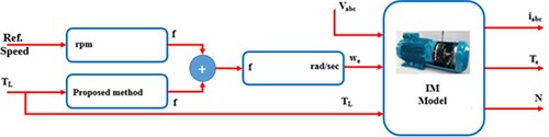
Table 1. Parameters of IM.

Parameters	Value	Unit
Rs	4.85	Ω
Rr	3.81	Ω
Ls	0.274	H
Lr	0.274	H
Lm	0.258	H
j	0.031	kgm^2
P	1.5	kW
p	4	–
we	1500	rpm

Here; R_s: Stator resistance, R_r: Rotor resistance, L_s: Stator inductance, L_r: Rotor inductance, L_m: Mutual inductance, j: Inertia, P: Power of the motor, p: number of poles.

2.3. Suggested curve fitting techniques

Generally, the data obtained as a result of experimental studies are point values. There is no continuous function definition between the data. In this sense, the data (x₁, y₁), … , (x_i, y_i) are given or obtained as pairs of points. Here, it is desired to find the f(x) function such that f(x_i) ≈ y_i for every i = 1, … , n. The process of determining another function closest to the function at given point values or searching for new functions that can facilitate real calculations is called “curve fitting”. Although it is seen that many methods are used in the literature, Polynomial, Fourier and Gaussian curve fitting methods are emphasized in this study. The methods proposed in this study are described below [49,51].

2.3.1. Polynomial curve fitting

In general, the expression for a polynomial of degree i is as follows. (3) $\begin{array}{l}f(x)=a_0+a_{1}x+a_2{x}^2+a_3{x}^3+\dots +a_i{x}^i\\ =a_0+\sum _{k=1}^i{a}_k{x}^k\end{array}$(3) Here, it is necessary to determine the most suitable coefficients for the curve depending on the data. The curve that gives the f(x) values with the minimum error in the equation is described as the “best” curve. The following equation is used for the error. (4) $\begin{array}{l}e=\sum _{}^{}{d}_i^2\\ =(y_1-f(x_1){)}^2+(y_2-f(x_2){)}^2+(y_3-f(x_3){)}^2\\ =\sum _{i=1}^n{(y_i-f(x_i))}^2\end{array}$(4)

Where n is the number of data points (each data point is an x, y pair). f(x) is the function that defines our optimal polynomial curve. The error equation can be written as: (5) $e=\sum _{i=1}^n(y_i-(a_0+\sum _{j=0}^k{a}_j{x}^j){)}^2$(5)

To find the minimum of this error function, its derivative is taken. Once the error is determined, an equation for the slope is obtained. The minimum error here indicates that the slope is “zero”. The unknown arises according to the degree of the polynomial. Assuming there are k unknowns, there will be unknowns such as a₀, a₁, … , a_k. Here, the derivative of each equation is taken separately. Unknowns are obtained by transforming the obtained equations into matrix form. (6) $\begin{array}{l}\left[\begin{array}{ccccc}n& \sum _{}^{}{x}_i& \sum _{}^{}{x}_i^2& \cdots & \sum _{}^{}{x}_i^j\\ \sum _{}^{}{x}_i& \sum _{}^{}{x}_i^2& \sum _{}^{}{x}_i^3& \cdots & \sum _{}^{}{x}_i^{j+1}\\ \sum _{}^{}{x}_i^2& \sum _{}^{}{x}_i^3& \sum _{}^{}{x}_i^4& \cdots & \sum _{}^{}{x}_i^{j+2}\\ ⋮& ⋮& ⋮& & ⋮\\ \sum _{}^{}{x}_i^j& \sum _{}^{}{x}_i^{j+1}& \sum _{}^{}{x}_i^{j+2}& \cdots & \sum _{}^{}{x}_i^{j+j}\end{array}\right]=A\\ \left[\begin{array}{c}{a}_0\\ a_1\\ a_2\\ ⋮\\ a_j\end{array}\right]=x,\left[\begin{array}{c}\sum y_i\\ \sum x_i{y}_i\\ \sum x_i^2{y}_i\\ ⋮\\ \sum x_i^j{y}_i\end{array}\right]=B\end{array}$(6) (7) $\begin{array}{l}A\ast x=B\\ x=A^{-1}\ast B\end{array}$(7)

2.3.2. Fourier curve fitting

The Fourier Series is the trigonometric expression of functions in terms of sine and cosine functions. Most of the single-valued functions that occur in practice can be expressed as a Fourier series in terms of sines and cosines.

Fourier series; It is a function f(x) in the range k ≤ x ≤ k + 2π. In this case, the general expression is; (8) $f(x)=\frac{a_0}{2}+\sum _{n=1}^{\mathrm{\infty }}(a_n\cos nx+b_n\sin nx)$(8) Here, (9) $\begin{array}{l}{a}_0={\displaystyle \frac{1}{\pi }}{\int }_k^{k+2\pi }f(x)dx\\ a_n={\displaystyle \frac{1}{\pi }}{\int }_k^{k+2\pi }f(x)\cos nxdx\\ b_n={\displaystyle \frac{1}{\pi }}{\int }_k^{k+2\pi }f(x)\sin nxdx\end{array}$(9)

The given expressions a₀, a_n, b_n are known as Euler equation. Here, the unknown occurs according to the number of terms. The unknowns are obtained by solving the Euler equations.

2.3.3. Gaussian curve fitting

The Gaussian model is adapted to the peaks and expressed as follows. (10) $y=\sum _{i=1}^n{a}_i{exp}^{[-{(x-b_i/c_i)}^2]}$(10) Here a is the amplitude, b is centre of gravity or position, c is the peak width. n is the appropriate number of peaks depending on 1 ≤ n ≤ 8. The solution is obtained according to the number of terms. For example, the following equation is used to solve a 2-term Gaussian equation. (11) $\begin{array}{rl}y& =f(x)=a_1{\exp }^{[-{(x-b_1/c_1)}^2]}+a_2{\exp }^{[-{(x-b_2/c_2)}^2]}\\ & +a_3{\exp }^{[-{(x-b_3/c_3)}^2]}\end{array}$(11)

The unknowns are obtained by transforming the given equation into matrix form. Thus, the curve equation closest to the solution of the problem is obtained.

3. Studies performed and findings obtained

3.1. Scalar control and simulink test studys

The simulation study made in the Matlab/Simulink program is given in Figure 2. The SC method was applied while detecting the speed error at different torque values of the motor.

Figure 2. Scalar speed control of IM.

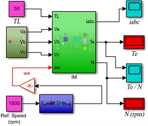
According to Figure 2, the nominal speed of the IM was determined as 1500 rpm and the variation of the speed according to the torque that may occur in the motor was examined. Thus, the loss of rotation of the motor speed was determined. The additional frequency values required to eliminate the loss of speed were determined by the tests carried out. The obtained values are given in Table 2.

Table 2. Additional frequency values required.

N (rpm)	Torq (Nm)	Δf (Hz)
1500	0	0
1500	5	0.15
1500	10	0.3
1500	15	0.45
1500	20	0.6
1500	25	0.8
1500	30	0.99
1500	35	1.19
1500	40	1.4
1500	45	1.63
1500	50	1.91

The additional frequency (Δf) values given in Table 2 are the additional frequency values required for the motor to reach 1500 rpm per minute. The frequency value required for torque 0 Nm and 1500 rpm is 50 Hz. As the torque value increases, losses occur in the speed value. The frequency is increased to tolerate these losses. N parameter given in Table 2 is the desired speed value. The speed loss (speed error) and error percentage experienced as the torque increases are given in Table 3.

Table 3. Speed error values.

Torq (Nm)	Ref. Speed N (rpm)	SC Obtained N (rpm)	Error N (%)
0	1500	1500	0.00%
5	1500	1492	0.53%
10	1500	1483	1.13%
15	1500	1474	1.73%
20	1500	1465	2.33%
25	1500	1455	3.00%
30	1500	1446	3.60%
35	1500	1436	4.27%
40	1500	1425	5.00%
45	1500	1414	5.73%
50	1500	1403	6.47%

When Table 3 is examined, speed errors and error percentage are seen according to the increasing torque values of the motor. The points used in obtaining the curves are the torque and Δf values given in Table 2. In the equations created, x values correspond to torque values, y = f(x) values correspond to Δf values. The curve equations and coefficients are as follows. The error N given in Table 3 is the speed error percentage of the motor.

3.2. Polynomial method

The calculations required for the polynomial were performed with the curve fitting toolbox. The optimal curve equation was obtained with a 5th degree polynomial. The equation of the polynomial and the calculated coefficients are as follows. (12) $f(x)=p_1{x}^5+p_2{x}^4+p_3{x}^3+p_4{x}^2+p_{5}x+p_6$(12)

The coefficients calculated here are; $\begin{array}{rl}{p}_1& =1.385e^{-08},p_2=-1.684e^{-06},p_3=7.362e^{-05},\\ p_4& =-0.001143,p_5=0.0353,p_6=-0.001276\end{array}$

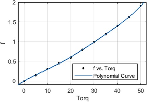
The graph obtained according to the polynomial equation curve is given in Figure 3. In Figure 3 f represents Δf.

Figure 3. Polynomial equation curve.

3.3. Fourier method

Calculations required for Fourier were performed with the Curve fitting toolbox. The number of terms of the optimal curve equation is 3. The Fourier equation and the calculated coefficients are as follows. (13) $\begin{array}{rl}f(x)& =a_0+a_1\cos (xw)+b_1\sin (xw)+a_2\cos (2xw)\\ & +b_2\sin (2xw)+a_3\cos (3xw)+b_3\sin (3xw)\end{array}$(13)

The coefficients calculated here are; $\begin{array}{rl}{a}_0& =1.051,a_1=-1.079,b_1=-0.2868,\\ a_2& =-0.06152,b_2=0.3523,a_3=0.08931,\\ b_3& =0.009753,w=0.06139\end{array}$

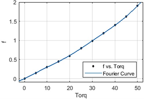
The graph obtained according to the Fourier equation curve is given in Figure 4.

Figure 4. Fourier equation curve.

3.4. Gaussian method

The calculations required for Gaussian were performed with the Curve fitting toolbox. The number of terms of the optimal curve equation is 3. The Gaussian equation and the calculated coefficients are as follows. (14) $\begin{array}{rl}f(x)& =a_1{\exp }^{[-{(x-b_1/c_1)}^2]}+a_2{\exp }^{[-{(x-b_2/c_2)}^2]}\\ & +a_3{\exp }^{[-{(x-b_3/c_3)}^2]}\end{array}$(14)

The coefficients calculated here are; $\begin{array}{l}{a}_1=2.197,b_1=60.11,c_1=23.93,\\ a_2=0.5561,b_2=28.42,c_2=14.99,\\ a_3=0.1633,b_3=12.01,c_3=7.837\end{array}$

The graph obtained according to the Gaussian equation curve is given in Figure 5.

Figure 5. Gaussian equation curve.

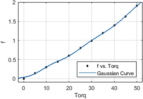
In addition, the best fit values calculated are given in Table 4. Here, SSE: Sum of Squares Error, RMSE: Root Mean Squared Error.

Table 4. Best fit values.

	Polynomial	Fourier	Gaussian
SSE	0.0002315	0.0001397	0.001902
R-Square	0.9999	1	0.9995
Adjusted R-Square	0.9999	0.9999	0.9976
RMSE	0.006805	0.006823	0.03084

3.5. Test results

The results obtained from the simulation tests are given in Figures 6–8. Here, the results of Polynomial Control (PC), Fourier Control (FC) and Gaussian Control (GC) methods are shown, respectively.

Figure 6. PC_IM results (25 Nm – 1500 rpm).

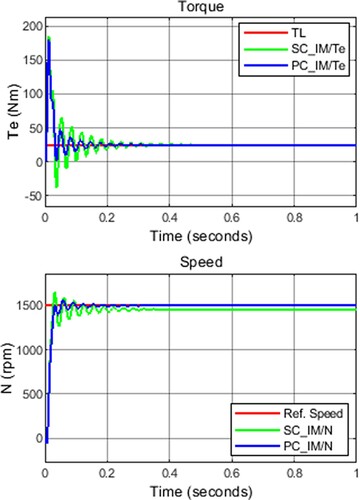
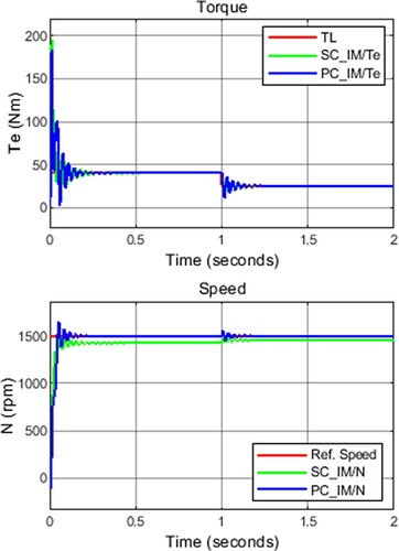
Figure 7. FC_IM results (25 Nm – 1500 rpm).

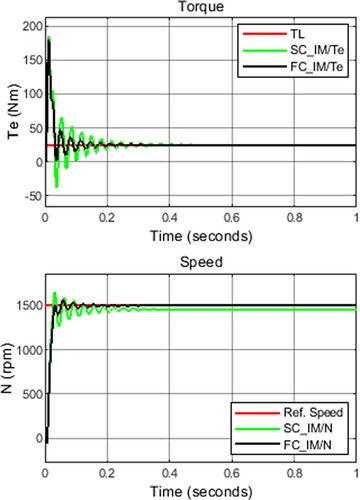
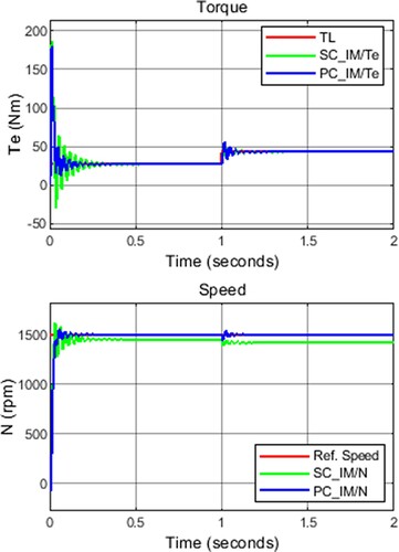
Figure 8. GC_IM results (25 Nm – 1500 rpm).

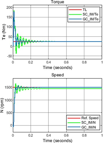
When the PC graphics given in Figure 6 are examined, it is seen that the torque value is more optimal and the expected speed value is obtained. When the FC graphics given in Figure 7 are examined, it is seen that the torque value is more optimal and the expected speed value is obtained. When the GC graphics given in Figure 8 are examined, it is seen that the torque value is more optimal and the expected speed value is obtained.

In Table 5, the test results performed with the PC_IM method for all experimental values are given. In the table, 1501 rpm with 5 Nm torque and 1499 rpm with 45 Nm torque are obtained. The PC_IM method produced incorrect results on two values.

Table 5. PC_IM test results.

Torq (Nm)	Ref. Speed N (rpm)	PC Obtained N (rpm)	Error N (%)
0	1500	1500	0.00%
5	1500	1501	−0.07%
10	1500	1500	0.00%
15	1500	1500	0.00%
20	1500	1500	0.00%
25	1500	1500	0.00%
30	1500	1500	0.00%
35	1500	1500	0.00%
40	1500	1500	0.00%
45	1500	1499	0.07%
50	1500	1500	0.00%

In Table 6, the test results performed with the FC_IM method for all experimental values are given. In the table, 1499 rpm with 20 Nm torque, 1501 rpm with 30 Nm torque, 1499 rpm with 45 Nm torque are obtained. The FC_IM method produced incorrect results on three values.

Table 6. FC_IM test results.

Torq (Nm)	Ref. Speed N (rpm)	FC Obtained N (rpm)	Error N (%)
0	1500	1500	0.00%
5	1500	1500	0.00%
10	1500	1500	0.00%
15	1500	1500	0.00%
20	1500	1499	0.07%
25	1500	1500	0.00%
30	1500	1501	−0.07%
35	1500	1500	0.00%
40	1500	1500	0.00%
45	1500	1499	0.07%
50	1500	1500	0.00%

In Table 7, the test results performed with the GC_IM method for all experimental values are given. In the table, 1502 rpm with 0 Nm torque, 1499 rpm with 5 Nm torque, 1501 rpm with 10 Nm torque, 1499 rpm with 20 Nm torque, 1501 rpm with 30 Nm torque, 1499 rpm with 40 Nm torque are obtained. The GC_IM method produced 6 incorrect results.

Table 7. GC_IM test results.

Torq (Nm)	Ref. Speed N (rpm)	GC Obtained N (rpm)	Error N (%)
0	1500	1502	−0.13%
5	1500	1499	0.07%
10	1500	1501	−0.07%
15	1500	1500	0.00%
20	1500	1499	0.07%
25	1500	1500	0.00%
30	1500	1501	−0.07%
35	1500	1500	0.00%
40	1500	1499	0.07%
45	1500	1500	0.00%
50	1500	1500	0.00%

When Figures 6–8 are examined together, it is seen that similar results are obtained. It can be said that numerical solutions produce similar solutions. This can be explained by the fact that the values given in Table 5 are close to each other.

 Figures 9 and 10 show the performance of the IM versus variable torque values. Since the proposed methods produce similar results, the responses of the system against variable torque values are evaluated only according to the PC_IM method.

Figure 9. PC_IM results for stepped torque values (25–40 Nm).

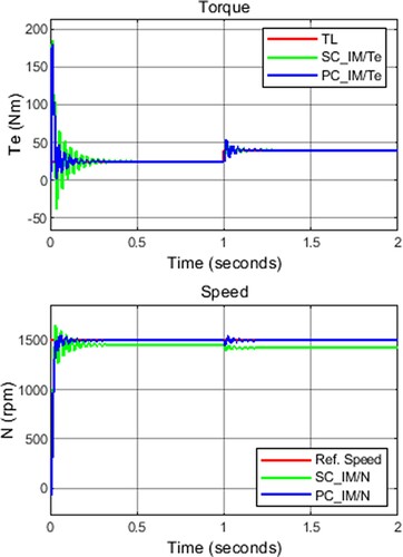
Figure 10. PC_IM results for stepped torque values (40–25 Nm).

The performance of the motor with torque values of 25 and 40 Nm is shown in Figure 9. The motor started with 25 Nm and increased to 40 Nm in 1st second. According to the SC method, the speed of the IM was measured to be 1455 rpm at 25 Nm and 1425 rpm at 40 Nm. According to the PC method, the IM speed is 1500 rpm at both torque values.

The performance of the motor with torque values of 40 and 25 Nm is shown in Figure 10. The motor started with 40 Nm and was reduced to 25 Nm in 1st second. According to the SC method, the speed of the IM was measured to be 1425 rpm at 40 Nm and 1455 rpm at 25 Nm. According to the PC method, the IM speed is 1500 rpm at both torque values.

In Figure 11, apart from the test values given in Table 2, test results for two different torque values are given. Here, the performance of the IM for randomly selected 27 and 43 Nm torque values is examined. The speed of the IM was measured as 1451 rpm at 27 Nm and 1419 rpm at 43 Nm according to the SC method. According to the PC method, the IM speed is 1500 rpm at both torque values.

Figure 11. PC_IM results for stepped torque values (27–43 Nm).

4. Conclusion

In this study, in which scalar velocity control was performed using different curve fitting methods for IM, the following results were obtained.

• The proposed PC_IM, FC_IM and GC_IM techniques have increased the rate control performance of IM. In this sense, they produced more successful results than SC_IM (Figures 6–8).

• When the proposed techniques were evaluated among themselves, it was seen that all techniques responded to torque changes in a shorter time than the SC_IM method (Figures 6–8).

• It is understood that the proposed methods are more successful in gradual torque increase (Figures 9 and 10).

• It was observed that the proposed methods were more successful in the tests performed with values other than the data obtained with the experimental results (Table 2) (Figure 11).

• When the proposed methods are evaluated in themselves, it can be said that the PC_IM method produces the most successful results. The worst results belong to the GC_IM method. In this sense, when Table 7 is examined, six erroneous results are seen. This is two in PC_IM and three in FC_IM (Tables 5 and 6).

• When Tables 4–6 are examined, it is seen that all errors are at a negligible level and the rate of errors is between 0.07% and 0.13%.

In this study, curve fitting methods, one of the numerical solution methods, were used directly under the control of a controller and it was determined that the results could make positive contributions to the literature. Considering the studies in this field, it is understood that many more studies can be done.

This study shows that numerical solution methods can be used as a controller. Different solutions can be produced in different applications. These proposed methods can be used in the control of other electric motors and different studies can be done on these issues.

Disclosure statement

No potential conflict of interest was reported by the author(s).

References

- Trzynadlowski AM. The field orientation principle in control of induction motors. Switzerland: Springer Science & Business Media; 2013.
- Trzynadlowski AM. Control of induction motors. Nevada: Elsevier; 2000.
- Musa EAM, Yonis AI, Ali GGT, et al. Speed control of three phase induction motor using variable frequency drive. Ahmedabad, India: Sudan University Of Science & Technology; 2020.
- Abu-Rub H, Iqbal A, Guzinski J. High performance control of AC drives with Matlab/Simulink. United Kingdom: John Wiley & Sons; 2021.
- Theraja B. A textbook of electrical technology. New Delhi: S. Chand Publishing; 2008.
- Saghafinia A, Ping HW, o MJIR, et al. High performance induction motor drive using hybrid fuzzy-pi and pi controllers: A review. Int Rev Electric Eng. 2010;5(5):2000–2012.
- Patel S. Speed control of three-phase induction motor using variable frequency drive. Long Beach: California State University; 2018.
- Wu B, Narimani M. High-power converters and AC drives. New York: John Wiley & Sons; 2017.
- Jain JK, Ghosh S, Maity S, et al. PI controller design for indirect vector controlled induction motor: a decoupling approach. ISA Trans. 2017;70:378–388.
- Ammar HH, Azar AT, Tembi TD, et al. Design and implementation of fuzzy PID controller into multi agent smart library system prototype. International Conference on Advanced Machine Learning Technologies and Applications, Springer, 2018. p. 127–137.
- Wang K, Lorenz RD, Baloch NA. Improvement of back-EMF self-sensing for induction machines when using deadbeat-direct torque and flux control. IEEE Trans Ind Appl. 2017;53(5):4569–4578.
- Zhang Y, Yin Z, Li G, et al. A novel speed estimation method of induction motors using real-time adaptive extended Kalman filter. J Electric Eng Technol. 2018;13(1):287–297.
- Xin Z, Zhao R, Blaabjerg F, et al. An improved flux observer for field-oriented control of induction motors based on dual second-order generalized integrator frequency-locked loop. IEEE J Emerg Sel Top Power Electron. 2016;5(1):513–525.
- Zhou Z, Yu J, Yu H, et al. Neural network-based discrete-time command filtered adaptive position tracking control for induction motors via backstepping. Neurocomputing. 2017;260:203–210.
- Wang N, Yu H, Liu X. DTC of induction motor based on adaptive sliding mode control. Chinese Control and Decision Conference (CCDC): IEEE, 2018. p. 4030–4034.
- Lftisi F, Rahman M. A novel finite element controller map for intelligent control of induction motors. 8th IEEE Annual Information Technology, Electronics and Mobile Communication Conference (IEMCON): IEEE, 2017, p. 18–24.
- Nozaki Y, Koseki T, Masada E. Analysis of linear induction motors for HSST and linear metro using finite difference method. Proc. LDIA2005. 2005: 168–171.
- Zhao J, Bose BK. Evaluation of membership functions for fuzzy logic controlled induction motor drive. IEEE 2002, 28th Annual Conference of the Industrial Electronics Society. IECON 02, Vol. 1: IEEE, 2002. p. 229–234.
- Rashed M, MacConnell PF, Stronach AF. Nonlinear adaptive state-feedback speed control of a voltage-fed induction motor with varying parameters. IEEE Trans Ind Appl. 2006;42(3):723–732.
- Paice DA. Induction motor speed control by stator voltage control. IEEE Trans Power Appar Syst. 1968;2:585–590.
- Feng Y, Zhou M, Han F, et al. Speed control of induction motor servo drives using terminal sliding-mode controller. Advances in variable structure systems and sliding mode control—theory and applications: Springer, 2018, p. 341–356.
- Guo Y, Wang X, Guo Y, et al. Speed-sensorless direct torque control scheme for matrix converter driven induction motor. J Eng. 2018;2018(13):432–437.
- Lin F-J, Shen P-H, Hsu S-P. Adaptive backstepping sliding mode control for linear induction motor drive. IEE Proc Electr Power Appl. 2002;149(3):184–194.
- Kubota H, Matsuse K, Nakano T. DSP-based speed adaptive flux observer of induction motor. IEEE Trans Ind Appl. 1993;29(2):344–348.
- Khlaief A, Saadaoui O, Abassi M, et al. Open circuit fault detection and FTC for sensorless PMS motor control based on the back-EMF SMO. Int J Electron. 2020;108(2):1–20.
- Li J, Ren H-P, Zhong Y-R. Robust speed control of induction motor drives using first-order auto-disturbance rejection controllers. IEEE Trans Ind Appl. 2014;51(1):712–720.
- Irmak E, Seyfettin V. Asenkron motorlarda frekans değişimi ile hiz kontrolü deneyinin bilgisayar üzerinden gerçekleştirilmesi. Gazi Üniversitesi Mühendislik Mimarlık Fakültesi Dergisi. 2011;26(1):57–62.
- Otkun O, Doğan R, Akpinar A. Neural network based scalar speed control of linear permanent magnet synchronous motor, 2015.
- Sharma K, Agrawal A, Bandopadhaya S. Fuzzy logic controlled variable frequency drives. Harmony Search and Nature Inspired Optimization Algorithms: Springer, 2019, p. 1153–1164.
- Pongfai J, Assawinchaichote W. Optimal PID parametric auto-adjustment for BLDC motor control systems based on artificial intelligence. International Electrical Engineering Congress (iEECON), IEEE, 2017, p. 1–4.
- Stoer J, Bulirsch R. Introduction to numerical analysis. Cambridge, Massachusetts, USA: Springer Science & Business Media; 2013.
- Lindfield G, Penny J. Numerical methods: using MATLAB. Hoboken, USA: Academic Press; 2018.
- Kobayashi H, Seo Y, Ogawa K, et al. Numerical analysis and experiment for stress wave propagation in two connected cylindrical bodies with different cross-sectional area and same mechanical impedance. EPJ Web of Conferences, vol. 183: EDP Sciences, 2018, p. 01033.
- Otkun Ö. İndüksiyon motor denetiminde interpolasyon tekniklerinin kullanımı. Pamukkale Üniversitesi Mühendislik Bilimleri Dergisi. 2020;26(2):301–311.
- Otkun Ö. Newton–Raphson based scalar speed control and optimization of IM. Automatika. 2021;62(1):55–64.
- Khitrov A, Khitrov A, Kurnikov K. Parameter identification of induction motor drives. 28th International Workshop on Electric Drives: Improving Reliability of Electric Drives (IWED): IEEE, 2021, p. 1–5.
- Cirrincione M, Pucci M, Cirrincione G, et al. An adaptive speed observer based on a new total least-squares neuron for induction machine drives. IEEE Trans Ind Appl. 2006;42(1):89–104.
- Li Y, Lin H, Huang H, et al. Analysis and performance evaluation of an efficient power-fed permanent magnet adjustable speed drive. IEEE Trans Ind Electron. 2018;66(1):784–794.
- Torkaman H, Afjei E, Toulabi MS. New double-layer-per-phase isolated switched reluctance motor: concept, numerical analysis, and experimental confirmation. IEEE Trans Ind Electron. 2011;59(2):830–838.
- Pervin S, Siri Z, Uddin MN. Newton–Raphson based computation of id in the field weakening region of IPM motor incorporating the stator resistance to improve the performance. IEEE Industry Applications Society Annual Meeting: IEEE, 2012, p. 1–6.
- Gupta K, Ganguli S. Parameter identification and control of dc motor using curve fitting technique, 2014.
- Huang S, Chen Z, Huang K, et al. Maximum torque per ampere and flux-weakening control for PMSM based on curve fitting. 2010 IEEE Vehicle Power and Propulsion Conference: IEEE, 2010, p. 1–5.
- Si Y, Liu C, Zhang Z, et al. A novel interior permanent magnet synchronous motor drive control strategy based on off-line calculation and curve fitting. IEEE Applied Power Electronics Conference and Exposition (APEC): IEEE, 2020, p. 253–258.
- Pan J, Cheung NC, Yang J. High-precision position control of a novel planar switched reluctance motor. IEEE Trans Ind Electron. 2005;52(6):1644–1652.
- Xiaoyan W. Speed estimation of electric multiple unit traction motor based on curve fitting. J Electr Eng. 2015: 8.
- Khang H, Arkkio A. Parameter estimation for a deep-bar induction motor. IET Electr Power Appl. 2012;6(2):133–142.
- Sue S-M, Pan C-T. Voltage-constraint-tracking-based field-weakening control of IPM synchronous motor drives. IEEE Trans Ind Electron. 2008;55(1):340–347.
- Meshram P, Kanojiya RG. Tuning of PID controller using Ziegler-Nichols method for speed control of DC motor. IEEE-international conference on advances in engineering, science and management (ICAESM-2012): IEEE, 2012, p. 117–122.
- Greenspan D, Casulli V. Numerical analysis for applied mathematics, science, and engineering. Boca Raton: CRC Press; 2018.
- Enemuoh F, Okafor E, Onuegbu J, et al. Modelling, simulation and performance analysis of a variable frequency drive in speed control of induction motor. Int J Eng Inven. 2013;3(5):36–41.
- Matlab. MathWorks-Products and Services, Matlab/Simulink Product Family. [cited 2021 Jun 6]. Available from: https://se.mathworks.com/products.html?s_tid=gn_ps.