Online adaptive optimal tracking control for model-free nonlinear systems via a dynamic neural network

Abstract

This paper presents an online adaptive approximate solution for the optimal tracking control problem of model-free nonlinear systems. Firstly, a dynamic neural network identifier with properly designed weights updating laws is developed to identify the unknown dynamics. Then an adaptive optimal tracking control policy consisting of two terms is proposed, i.e. a steady-state control term is established to ensure the desired tracking performance at the steady state, and an optimal control term is proposed to ensure the optimal tracking error dynamics optimally. The composite Lyapunov method is used to analyse the stability of the closed-loop system. Two simulation examples are presented to demonstrate the effectiveness of the proposed method.

KEYWORDS:

• Dynamic neural network
• nonlinear systems
• nonlinear identifier
• adaptive control
• optimal control

1. Introduction

The basic idea of the classical adaptive control is to update the model parameter and control law directly or indirectly, such that the control error can be minimized. However, it is generally not optimal. On the other side, the main drawback of the classical optimal control approach lies in that the system dynamics must be precisely known for solving the Hamilton-Jacobi-Bellman (HJB) equation in an off-line manner [1]. Hence, by merging the knowledge from adaptive control and optimal control, the adaptive optimal control approach has been developed during the past decade and a survey of this research can be found in [2–4].

To develop an online adaptive optimal control, Werbos [5] introduced the general actor-critic (AC) framework for adaptive optimal control. The critic neural network (NN) approximates the evaluation function, mapping states to an estimated measure of the value function, whereas the NN approximates an optimal control law and generates the actions or control signals. Since then, various modifications to adaptive optimal control algorithms have been proposed as model-based methods (heuristic dynamic programming – HDP [6] and dual heuristic programming-DHP [7]) and model-free methods (action-dependent heuristic dynamic programming – ADHDP [8] and Q learning [9]). However, most of the previous works on adaptive optimal control have focused on discrete-time systems. The extensions of these adaptive optimal control research to continuous-time systems pose challenges in proving stability, convergence and ensuring the online updating law with model free [10].

Discretizinging the continuous time system is generally not accurate, especially for the high-dimensional systems that prohibit the learning process. Hence, the online policy iteration-based algorithms are proposed to solve the linear [11] and nonlinear [12] continuous-time infinite horizon optimal control problems, which involve synchronous adaptive of both actor and critic NN. Furthermore, ref. [10] extended the idea in refs. [11,12] by designing a novel AC-identifier architecture to approximate the HJB equation without the knowledge of system drift dynamics, but the knowledge of the input dynamics is required. The recent research in [13] cancels this requirement by using the experience iteration technique. Based on ref. [10], a simply identifier-critic structure-based optimal control method is proposed in [14,15], where just a critic NN is used to approximate the solution of the HJB equation and to calculate the optimal control action. In [16], an optimal control method for nonzero-sum differential games of continuous-time nonlinear systems is designed directly from the critic NN instead of the action-critic dual network, which greatly simplifies the algorithm architecture.

Most of the existing adaptive optimal research studies mainly focus on dealing with regulation problems rather than trajectory tracking problems. The combined consideration of two aspects can ensure not only the realization of trajectory tracking and stabilization but also satisfying the prescribed performance index (such as minimization of the trajectory error, fuel consumption, etc.). In [17] a new data-based iterative optimal learning control scheme is developed to solve a coal gasification optimal tracking control problem in the discrete-time domain. For continuous-time systems, linear quadratic tracking control of partially-unknown systems using reinforcement learning is present in [18] and a nonlinear approximately optimal trajectory tracking method with exact model information is developed in [19]. To relax the requirement of an explicit model, a steady-state control conjunction with an optimal control for nonlinear continuous-time systems is developed in [20], which stabilizes the error dynamics in an optimal way.

Most of the above-mentioned adaptive optimal control method is based on the affine nonlinear system, to the best of our knowledge, only [21] addressed the adaptive optimal control of unknown non-affine nonlinear systems in the discrete-time domain and [22] introduces an adaptive recursive control for the model-based non-affine nonlinear continuous system. The optimal control of an unknown non-affine nonlinear continuous-time system is still a challenging task, which is the motivation of this paper.

The main contributions of this paper are listed as follows.

• (1) The optimal tracking control of unknown non-affine nonlinear systems based on the critic identifier architecture is first proposed in this paper. Model-free property is achieved by a neuro identifier in conjunction with the novel updating laws for both the weights and the linear part matrix which is usually assumed to be a known Hurwitz matrix for the conventional black-box nonlinear system identification.

• (2) Adaptive optimal tracking control policy consisting of two terms is proposed, i.e. a steady-state control term is established to ensure the desired tracking performance at the steady state, and an optimal control term is proposed to ensure the optimal tracking error dynamics. Online solution of the optimal control term is obtained directly by a single critic NN to approximate the optimal cost function of the HJB equation instead of the conventional action-critic dual network, which greatly reduces complexity and saves calculation time. A novel learning law driven by filtered parameter error is proposed for critic NN. The stability of the entire closed-loop system is proved by the properly designed composite Lyapunov method.

The main organization of the paper is as follows. The problem formulation is given in Section 2. The DNN identifier is designed in Section 3. Then, the optimal control strategy, based on the critic-identifier architecture, is present in Section 4. Two simulation examples are presented to verify the proposed scheme in Section 5 and the conclusion is drawn in Section 6.

2. Problem formulation

Consider the following non-affine nonlinear continuous-time systems (1) $\dot{x}\left(t\right)=f\left(x\right(t),u(t\left)\right)$(1) where $x\left(t\right)=\left(x_1\right(t),x_2(t),\dots ,x_n(t){)}^T\in R^n$ is the state vector, $u\left(t\right)=\left(u_1\right(t),u_2(t),\dots ,u_m(t){)}^T\in R^m$ is the control input vector and $f(\cdot )$ is an unknown continuous nonlinear smooth function for $x\left(t\right)$ and $u\left(t\right)$.

The objective of the optimal tracking control problem is to design an optimal controller (1) to ensure that the state vector $x\left(t\right)$ tracks the specified trajectory $x_r\left(t\right)$ and minimize the infinite horizon performance cost function as follows: (2) $V\left(e\right(t\left)\right)={\int }_t^{\mathrm{\infty }}r\left(e\right(\tau ),u_e\left(e\right(\tau \left)\right)d\tau$(2) where the tracking error is defined as $e\left(t\right)=x\left(t\right)-x_r\left(t\right)$, the utility function with symmetric positive definite matrices $Q$ and $R$ is defined as $r\left(e\right(t),u(t\left)\right)=e^T\left(t\right)Qe\left(t\right)$ $+u_{}^T\left(t\right)Ru\left(t\right)$.

From the basic optimal control theory, we define the Hamiltonian of (1) as (3) $\begin{array}{rl}H(e,u_e,V)& =V_e^T\left[f\right(x\left(t\right),u\left(t\right)\left)\right]+e^{T}Qe\\ & +u_{}^T\left(t\right)Ru\left(t\right)\end{array}$(3) where $V_e\stackrel{\mathrm{\Delta }}{=}\frac{\mathrm{\partial }V}{\mathrm{\partial }x}$ denotes the partial derivative of the cost function $V\left(e\right(t\left)\right)$ with respect to $e\left(t\right)$.

The optimal cost function $V^{\ast }\left(e\right(t\left)\right)$ is given as (4) $V^{\ast }\left(e\right(t\left)\right)=min\underset{u\in \psi \left(\mathrm{\Omega }\right)}{min}{\int }_t^{\mathrm{\infty }}r\left(e\right(\tau ),u_e\left(e\right(\tau \left)\right)d\tau$(4) and it satisfies the HJB equation (5) $\begin{array}{rl}H(e,u^{\ast },V^{\ast })& =V_e^{\ast T}\left[f\right(x\left(t\right),u^{\ast }\left(t\right)\left)\right]+e^T\left(t\right)Qe\left(t\right)\\ & +u_{}^{\ast T}\left(t\right)R{u}^{\ast }\left(t\right)\end{array}$(5) where the control $u$ is defined to be admissible for (2) on a compact set $\mathrm{\Omega }\in R^n$, denoted by $u\in \psi \left(\mathrm{\Omega }\right)$.

Theoretically, the optimal control for nonlinear system (1) can be obtained from Equations (4) and (5). However, optimal control cannot be obtained in practical systems due to two reasons: 1). The optimal cost function $V^{\ast }\left(e\right(t\left)\right)$ should be obtained by solving the HJB equation (5). However, it is usually difficult to solve the high-order nonlinear partial differential equation (PDE) for general nonlinear systems via analytical methods. Moreover, the unknown nonlinear dynamic $f(\cdot )$ makes the solution unavailable for HJB Equation (2). The idea of optimal control $u^{\ast }\left(t\right)$ cannot be derived by solving $\frac{\mathrm{\partial }H(e,u^{\ast },V^{\ast })}{\mathrm{\partial }{u}^{\ast }}=\text{0}$ due to the unavailability of $V^{\ast }\left(e\right(t\left)\right)$.

In this paper, we develop a critic-identifier to solve the optimal control of an unknown non-affine nonlinear continuous-time system, all the learning processes can be updated online.

3. Adaptive model-free identifier

We employ the following dynamic neural network (DNN) model to approximate the nonlinear dynamic system (1) (6) $\dot{\hat{x}}\left(t\right)=A\hat{x}\left(t\right)+W_1\sigma \left(V_1\left[\hat{x}\left(t\right)\right]\right)+W_2\varphi \left(V_2\left[\hat{x}\left(t\right)\right]\right)u\left(t\right)$(6) where $\hat{x}\left(t\right)\in R^n$ is the state of the DNN, $W_1\in R^{n\times m},W_2\in R^{m\times n}$ are the weights in the output layers, $W_1\in R^{n\times m},W_2\in R^{m\times n}$ are the weights in the hidden layer, $A\in R^{n\times n}$ is the matrix for the linear part of NNs, $u\left(t\right)=(u_1\left(t\right),u_2\left(t\right),\dots ,u_k\left(t\right),0,\dots ,0{)}^T\in R^m$ is the control input, the active function $\sigma (\cdot )$ (as well as $\varphi (\cdot )$) is the sigmoidal vector function which is defined as $\sigma (\cdot )=a/(1+e^{-bx})-c$, where a, b and c are constants.

Remark

If we define $W=\left[W_1,W_2\right],$ $\mathrm{\Xi }=\left\{\sigma \right(V_{\text{1}}\left[\hat{x}\right(t\left)\right]),\phi (V_{\text{2}}\left[\hat{x}\right(t\left)\right]\left)u\right(t\left)\right\}$, then (6) can be written as $\dot{\hat{x}}\left(t\right)=A\hat{x}\left(t\right)+W\mathrm{\Xi }$. It has been proved in [23] that DNN with the form $\dot{\hat{x}}\left(t\right)=A\hat{x}\left(t\right)+W\mathrm{\Xi }$ can approximate the nonlinear system (1) to any degree of accuracy if the hidden layer $V$ is large enough. Here, to simplify the analysis process, we consider the simplest structure (i.e. $m=n,V=I,\varphi (\cdot )=I$).

Then the nonlinear system (1) can be modelled by the DNN as follows: (7) $\dot{x}\left(t\right)=A^{\ast }x\left(t\right)+{W_1}^{\ast }\sigma \left(x\left(t\right)\right)+{W_2}^{\ast }u\left(t\right)+{\xi }_1$(7) where $A^{\ast }$, ${W_1}^{\ast },{W_2}^{\ast }$ are the nominal unknown matrices and ${W_1}^{\ast },{W_2}^{\ast }$ are bounded as ${W_1}^{\ast }{{\mathrm{\Lambda }}_1}^{-1}{W_1}^{\ast T}\le \overline{W_1},{W_2}^{\ast }{{\mathrm{\Lambda }}_2}^{-1}{W_2}^{\ast T}\le \overline{W_2}$ (${{\mathrm{\Lambda }}_1}^{-1},{{\mathrm{\Lambda }}_2}^{-1}$ are any positive definite symmetric matrices), and ${\xi }_1$ is regarded as the modelling error or disturbance and is assumed to be bounded.

Assumption

The identification error is defined by $\mathrm{\Delta }x=x\left(t\right)-\hat{x}\left(t\right)$. The difference in the activation function $\tilde{\sigma }=\sigma \left(x\left(t\right)\right)-\sigma \left(\hat{x}\left(t\right)\right)$ satisfies the generalized Lipshitz condition ${\tilde{\sigma }}^T\mathrm{\Lambda }\tilde{\sigma }<[\mathrm{\Delta }x{]}^{T}D\left[\mathrm{\Delta }x\right]=\mathrm{\Delta }{x}^{T}D\mathrm{\Delta }x$, and $D=D^T>0$ is the known normalizing matrices.

Then from (6) and (7), we can obtain the error dynamic equation (8) $\begin{array}{rl}\mathrm{\Delta }\dot{x}& =A^{\ast }\mathrm{\Delta }x+\tilde{A}\hat{x}\left(t\right)+{W_1}^{\ast }\tilde{\sigma }+{\tilde{W}}_1\sigma \hat{x}\left(t\right)\\ & +{\tilde{W}}_{2}u\left(t\right)+{\xi }_1\end{array}$(8) where $\tilde{A}=A^{\ast }-A$ ${\tilde{W}}_1={W_1}^{\ast }-W_1,{\tilde{W}}_2={W_2}^{\ast }-W_2,$

Lemma

[24]

$A\in {\mathrm{\Re }}^{n\times n}$ is a Hurwitz matrix, $R,Q\in {\mathrm{\Re }}^{n\times n}$ $R=R^T>0$,$Q=Q^T>0$ if $\left(A,R^{1/2}\right)$ is controllable, $\left(A,Q^{1/2}\right)$ is observable and $A^T{R}^{-1}A-Q\ge$ $\frac{1}{4}\left(A^T{R}^{-1}-R^{-1}A\right)R\left(A^T{R}^{-1}-R^{-1}A\right)$ is satisfied, the algebraic Riccati equation $A^{T}X+XA+XRX+Q=0$ has a unique positive definite solution $X=X^T>0$.

Theorem

Consider the identification scheme (6) for (1), the following updating law (9) $\begin{array}{rl}\dot{A}& =-k_1\mathrm{\Delta }x{\hat{x}}^T,{\dot{W}}_1=-k_2\mathrm{\Delta }x{{\sigma }_1}^T\left(\hat{x}\right),\\ {\dot{W}}_2& =-k_3\mathrm{\Delta }x{u}^T\end{array}$(9) where k_1, k₂ and k₃ are positive constants, can guarantee the following stability properties:

1. For a precise identifier case i.e. ${\xi }_1=0$ ${\hat{W}}_{1,2},\hat{A}\in L_{\mathrm{\infty }},\mathrm{\Delta }x\in L_2\cap L_{\mathrm{\infty }},\underset{t\to \mathrm{\infty }}{lim}\mathrm{\Delta }x=0.$

2. For bounded modelling error and disturbances i.e. ${\xi }_1\le \overline{{\xi }_1}$ $\mathrm{\Delta }x,{\hat{W}}_{1,2},\hat{A}\in L_{\mathrm{\infty }}.$

Proof:

Consider the Lyapunov function candidate (10) $\begin{array}{rl}{L}_I& =\mathrm{\Delta }{x}^{T}P\mathrm{\Delta }x+\frac{1}{k_2}tr\left\{{\tilde{W}}_1^T{P}_x{\tilde{W}}_1\right\}+\frac{1}{k_3}tr\left\{{\tilde{W}}_2^T{P}_x{\tilde{W}}_2\right\}\\ & +\frac{1}{k_1}tr\left\{{\tilde{A}}^T{P}_x\tilde{A}\right\}\end{array}$(10)

Hence, differentiating (11) and using (8) yield (11) $\begin{array}{rl}{\dot{L}}_I& =\mathrm{\Delta }{x}^T({A^{\ast }}^{T}P+P{A}^{\ast })\mathrm{\Delta }x+2\mathrm{\Delta }{x}^{T}P\tilde{A}\hat{x}\\ & +2\mathrm{\Delta }{x}^{T}P{\tilde{W}}_1\sigma \left(\hat{x}\right)+2\mathrm{\Delta }{x}^{T}P{\tilde{W}}_{2}u\\ & +2\mathrm{\Delta }{x}^{T}P{W}_1^{\ast }\tilde{\sigma }+2\mathrm{\Delta }{x}^{T}P{\xi }_{\text{1}}+\frac{2}{k_1}tr\left\{{\dot{\tilde{A}}}^{T}P\tilde{A}\right\}\\ & +\frac{2}{k_2}tr\left\{{\dot{\tilde{W}}}_1^{T}P{\tilde{W}}_1\right\}+\frac{2}{k_3}tr\left\{{\dot{\tilde{W}}}_2^{T}P{\tilde{W}}_2\right\}\end{array}$(11) By using the updating laws (9) and taking the facts $\dot{\tilde{A}}=-\dot{A},{\dot{\tilde{W}}}_{1,2}=-{\dot{W}}_{1,2},$ into consideration, then (11) becomes (12) $\begin{array}{rl}{\dot{L}}_I& =\mathrm{\Delta }{x}^T({A^{\ast }}^{T}P+P{A}^{\ast })\mathrm{\Delta }x\\ & +2\mathrm{\Delta }{x}^{T}P{W}_1^{\ast }\tilde{\sigma }+2\mathrm{\Delta }{x}^{T}P{\xi }_{\text{1}}\end{array}$(12) Using the following matrix inequality (13) $X^{T}Y+(X^{T}Y{)}^T\le X^T{\mathrm{\Lambda }}^{-1}X+Y^T\mathrm{\Lambda }Y$(13) where $X,Y\in R^{j\times k}$ are any matrices and $\mathrm{\Lambda }\in R^{j\times k}$ is any positive definite matrix. From Assumption 3.1, one obtains (14) $\begin{array}{rl}2\mathrm{\Delta }{x}^{T}P{W}_1^{\ast }\tilde{\sigma }& \le \mathrm{\Delta }{x}^{T}P{W}_1^{\ast }{\mathrm{\Lambda }}^{-1}{W}_1^{\ast }P\mathrm{\Delta }x+{\tilde{\sigma }}^T\mathrm{\Lambda }\tilde{\sigma }\\ & \le \mathrm{\Delta }{x}^{T}P{\overline{W}}_{1}P\mathrm{\Delta }x+\mathrm{\Delta }{x}^{T}D\mathrm{\Delta }x\\ 2\mathrm{\Delta }{x}^{T}P{\xi }_1& \le \mathrm{\Delta }{x}^{T}P{\mathrm{\Lambda }}_{\xi }^{-1}P\mathrm{\Delta }x+{\xi }_1^T{\mathrm{\Lambda }}_{\xi }^{-1}{\xi }_1\end{array}$(14) Then substituting (14) into (12) obtains (15) $\begin{array}{rl}{\dot{L}}_I& \le \mathrm{\Delta }{x}^T\left(A^{\ast T}P+P{A}^{\ast }+P{\overline{W}}_{1}P+D+Q_0\right)\mathrm{\Delta }x\\ & -\mathrm{\Delta }{x}^T{Q}_0\mathrm{\Delta }x+\mathrm{\Delta }{x}^{T}P{\mathrm{\Lambda }}_{\xi }P\mathrm{\Delta }x+\mathrm{\Delta }{\xi }_1^T{\mathrm{\Lambda }}_{\xi }^{-1}\mathrm{\Delta }{\xi }_1\end{array}$(15) By defining $R={\overline{W}}_1,Q=D+Q_o$, then if we can select proper $Q_o$ so that $Q$ satisfies the conditions in Lemma 3.1, there exists matrix $P$ satisfying the equation $A^{\ast T}P+P{A}^{\ast }+PRP+Q=0$.

Hence (15) becomes (16) ${\dot{L}}_I\le -\mathrm{\Delta }{x}^T{Q}_0\mathrm{\Delta }x+\mathrm{\Delta }{x}^{T}P{\mathrm{\Lambda }}_{\xi }^{-1}P\mathrm{\Delta }x+\mathrm{\Delta }{\xi }_1^T{\mathrm{\Lambda }}_{\xi }^{-1}\mathrm{\Delta }{\xi }_1$(16) Case 1: For precise identifier case i.e. ${\xi }_1=0$, (16) becomes (17) ${\dot{L}}_I\le -\mathrm{\Delta }{x}^T{Q}_0\mathrm{\Delta }x\le -{\lambda }_{min}\left(Q_x\right)\Vert \mathrm{\Delta }x{\Vert }_{Q_x}^2\le 0$(17) From (17) we get $\mathrm{\Delta }x,{\hat{W}}_{1,2},\hat{A}\in L_{\mathrm{\infty }}$. Furthermore, from the error dynamics (8) we have $\dot{\mathrm{\Delta }}x\in L_{\mathrm{\infty }}$. By integrating (17) on both sides from 0 to ∞, we have ${\int }_0^{\mathrm{\infty }}[-{\lambda }_{min}(Q_x\left)||\mathrm{\Delta }x|{|}_{Q_x}^2\right]$ $\le \left[V_1\left(0\right)-V_1\left(\mathrm{\infty }\right)\right]<\mathrm{\infty }$, which implies that $\mathrm{\Delta }x\in L_2$. Since $\mathrm{\Delta }x\in L_2\cap L_{\mathrm{\infty }}$ and $\dot{\mathrm{\Delta }}x\in L_{\mathrm{\infty }}$, using Barbalat's Lemma we have $\underset{t\to \mathrm{\infty }}{lim}\mathrm{\Delta }x=0$.

Case 2: For bounded modelling error and disturbances i.e. ${\xi }_1\le {\overline{\xi }}_1$. Equation (16) can be represented as (18) $\begin{array}{rl}{\dot{L}}_I& \le -\mathrm{\Delta }{x}^T{Q}_0\mathrm{\Delta }x+\mathrm{\Delta }{x}^{T}P{\mathrm{\Lambda }}_{\xi }^{-1}P\mathrm{\Delta }x+\mathrm{\Delta }{\xi }_1^T{\mathrm{\Lambda }}_{\xi }^{-1}\mathrm{\Delta }{\xi }_1\\ & \le -\alpha (\Vert \mathrm{\Delta }x\Vert )+\text{β}\left(\Vert {\xi }_1\Vert \right)\end{array}$(18) where $\alpha (\Vert \mathrm{\Delta }x\Vert )=\left({\lambda }_{min}\left(Q_0\right)-{\lambda }_{max}\left(P{\mathrm{\Lambda }}_{\xi }P\right)\right)\Vert \mathrm{\Delta }x{\Vert }^2$ $\text{β}\left(||{\xi }_1||\right)={\lambda }_{max}\left({\mathrm{\Lambda }}_{\xi }^{-1}\right)||{\xi }_1|{|}^2$.

Since ${\alpha }_x$, ${\text{β}}_x$, ${\alpha }_y$, ${\text{β}}_y$ are $K_{\mathrm{\infty }}$ functions, $L_I$ is the ISS-Lyapunov function. Using Theorem 3.1 in [24], the dynamics of the identification error (8) is input to state stable, which implies $\mathrm{\Delta }x,W_{1,2},A\in L_{\mathrm{\infty }}$. This completes the proof of Theorem 3.1.

4. Optimal control design

In this section, adaptive optimal control is designed based on the DNN identifier. From Section 3, we know that a nonlinear system (1) can be represented by DNN with the updating law (9) as follows: (19) $\dot{x}=A\hat{x}+W_1\sigma \left(\hat{x}\right)+W_{2}u+{\xi }_1$(19) where the model error ${\xi }_1$ is still assumed to be bounded ${\xi }_1\le {\overline{\xi }}_1$. $\mathrm{\Delta }x$ and $W_{1,2}$ are bound as Theorem 3.1.

Then (19) can be further rewritten as (20) $\dot{x}=Ax+W_1\sigma \left(\hat{x}\right)+W_{2}u+{\xi }_2$(20) where ${\xi }_2={\xi }_1+A\hat{x}-Ax={\xi }_1-A\mathrm{\Delta }x$. For bounded ${\xi }_1$ and $\mathrm{\Delta }x$, ${\xi }_2$ is bounded as well i.e. ${\xi }_2\le {\overline{\xi }}_2$.

To achieve optimal tracking control, the control action u is designed as $u=u_r+u_e$ where $u_r$ is the steady-state control which ensures that the tracking error is at the steady state, and $u_e$ is the adaptive optimal control which is used to minimize the infinite horizon performance index function optimally. $u_r$ should be designed to compensate for the nonlinear dynamic in (20). Hence, let $u_r$ be (21) $u_r=W_2^{+}\left[{\dot{x}}_d-Ax-W_1\sigma \left(x\right)-Ke\right]$(21) where $e=x-x_r$ denotes the state tracking error, $K$ is the feedback gain and $W_2^{+}$ denotes the generalized inverse of $W_2$.

From (20) and (21), the error dynamic equation becomes (22) $\dot{e}=-Ke+W_2{u}_e+{\xi }_2$(22) In this case, the tracking problem with (20) is transferred to the regulator problem of (22). The adaptive optimal control $u_e$ is designed to stabilize (22) optimally. Hence rewrite the infinite horizon performance cost function (2) as (23) $V\left(e\right(t\left)\right)={\int }_t^{\mathrm{\infty }}r(e\left(\tau \right),u_e\left(e\right(\tau \left)\right)d\tau$(23) where $r\left(e,u_e\right)=e^{T}Qe+u_e^{T}R{u}_e$ is the utility function with the optimal control $u_e$.

According to the optimal regulator problem design in [25], an admissible control policy $u_e$ should be designed to ensure that the infinite horizon cost function (23) related to (22) is minimized. So, design the Hamiltonian of (22) as (24) $\begin{array}{rl}H\left(e,u_e,V\right)& =V_e^T\left[-Ke+W_2^{+}{u}_e+{\xi }_2\right]\\ & +e^{T}Qe+u_e^{T}R{u}_e\end{array}$(24) where $V_e=\frac{\mathrm{\partial }V\left(e\right)}{\mathrm{\partial }e}$ is the partial derivative of the value function with respect to e.

Then we define the optimal cost function as (25) $V^{\ast }\left(e\right(t\left)\right)=\underset{u_e\in \psi \left(\mathrm{\Omega }\right)}{min}({\int }_t^{\mathrm{\infty }}r\left(e\left(\tau \right),u_e\left(e\right(\tau \left)\right)d\tau \right)$(25) and it satisfies the following HJB equation (26) $\underset{u_e\in \psi \left(\mathrm{\Omega }\right)}{min}\left[H\left(e,u_e^{\ast },V^{\ast }\right)\right]=0$(26) The last optimal control value $u_e^{\ast }$ for (22) can be obtained by solving $\frac{\mathrm{\partial }H\left(e,u_e^{\ast },V^{\ast }\right)}{\mathrm{\partial }{u}_e^{\ast }}=0$ from (24) (27) $u_e^{\ast }=-\frac{1}{2}{R}^{-1}[W_2{]}^T\frac{\mathrm{\partial }{V}^{\ast }\left(e\right)}{\mathrm{\partial }e}$(27) where $V^{\ast }\left(e\right)$ is the solution of the HJB equation (26).

From (27), we can learn that the optimal control value $u_e^{\ast }$ is based on the optimal value function $V^{\ast }\left(e\right)$. However, it is difficult to solve the nonlinear partial differential HJB equation (26) to obtain $V^{\ast }\left(e\right)$. The usual method is to get the approximate solution via a critic NN as [4,5,25]. A single-layer NN will be used to approximate the optimal value function (28) $V^{\ast }\left(e\right)={\text{W}}_3^{\ast \text{T}}\varphi \psi \left(e\right)+{\xi }_3$(28) and its derivative is (29) $\frac{\mathrm{\partial }{V}^{\ast }\left(e\right)}{\mathrm{\partial }e}=\mathrm{\nabla }{\psi }^T\left(e\right){\text{W}}_3^{\ast }+\mathrm{\nabla }{\xi }_3$(29) where ${\text{W}}_3^{\ast }\in R^{\text{I}}$ is the nominal weight vector, $\psi \left(e\right)\in R^I$ is the active function and ${\xi }_3$ is the approximation error, I represents the number of neurons. $\mathrm{\nabla }\psi \left(e\right)=\frac{\mathrm{\partial }\psi \left(e\right)}{\mathrm{\partial }e}$ and $\mathrm{\nabla }{\xi }_3=\frac{\mathrm{\partial }{\xi }_3}{\mathrm{\partial }e}$ are the partial derivatives of $\psi \left(e\right)$ and ${\xi }_3$ with respect to e, respectively.

Assumption

The nominal weight vector ${\text{W}}_3^{\ast }$, the active function $\psi \left(e\right)$ and its derivative $\mathrm{\nabla }\psi \left(e\right)$ are all bound, i.e $||{\text{W}}_3^{\ast }||\le {\overline{W}}_3,\Vert \psi \left(e\right)\Vert \le {\overline{\psi }}_1,\Vert \mathrm{\nabla }\psi \left(e\right)\Vert \le {\overline{\psi }}_2$ $||\mathrm{\nabla }{\xi }_3||\le {\overline{\psi }}_3$.

Then substituting (28) with (27), one obtains (30) $u_e^{\ast }=-\frac{1}{2}{R}^{-1}{W}_2^T\left(\mathrm{\nabla }{\varphi }^T\left(e\right){\text{W}}_3^{\ast }+\mathrm{\nabla }{\xi }_3\right)$(30) The critic NN is approximated as (31) $V\left(e\right)={\text{W}}_3^{\text{T}}\varphi \left(e\right)$(31) where ${\text{W}}_3$ is the estimation of the nominal ${\text{W}}_3^{\ast }$.

Then the approximate optimal control can be obtained from (30) and (31) (32) $u_e=-\frac{1}{2}{R}^{-1}{W}_2^T\mathrm{\nabla }{\varphi }^T\left(e\right){\text{W}}_3$(32)

Remark

The available adaptive optimal control method is usually based on the dual NN architecture, where the critic NN and action NN are employed to approximate the optimal cost function and optimal control policy, respectively. The complicated structure and computational burden make it difficult for practical implantation. In the following, we will calculate the optimal control action directly from the critic NN instead of the action-critic dual network.

Substituting (28) with (24), one obtains (33) $\begin{array}{rl}0& ={\text{W}}_3^{\ast \text{T}}\mathrm{\nabla }\varphi \left(e\right)\left[-Ke+W_2^{+}{u}_e\right]\\ & +e^{T}Qe+u_e^{T}R{u}_e+{\xi }_{HJB}\end{array}$(33) where ${\xi }_{HJB}={\text{W}}_3^{\ast \text{T}}\varphi \left(e\right){\xi }_2+\mathrm{\nabla }{\xi }_3\left[-Ke+W_2^{+}{u}_e+{\xi }_2\right]$ is the residual HJB equation error due to the DNN identifier error ${\xi }_2$ and NN approximation error $\mathrm{\nabla }{\xi }_3$.

Then (33) can be written as the general identification form as (34) $Y=-{\text{W}}_3^{\ast \text{T}}X-{\xi }_{HJB}$(34) where $X=\mathrm{\nabla }\varphi \left(e\right)\left[-Ke+W_2^{+}{u}_e\right]$, $Y=e^{T}Qe+u_e^{T}R{u}_e$.

According to the least square method learning rules, one can get the estimation of nominal ${\text{W}}_3^{\ast }$ as ${\text{W}}_3=-(X{X}^T{)}^{-1}X{Y}^T$ in the case of residual HJB equation error equals zero. However, ${\xi }_{HJB}$ is not always zero and it is also difficult to finish the subsequent closed-loop stability analysis based on the least square method. Inspired by [14,26], we develop a novel robust estimation method of ${\text{W}}_3^{\ast }$. The following equation is used to identify (34) (35) $Y=-{\text{W}}_3^{\text{T}}X-{\xi }_{HJB1}$(35) where ${\xi }_{HJB}$ can be assumed to be the model error and unknown disturbance.

For (35), the filtered version of $Y$ is defined as (36) $\dot{z}=\tau z+Y,z\left(0\right)=0$(36) where ${\dot{L}}_o={{\tilde{W}}_3}^T{\mu }^{-1}{\dot{\tilde{W}}}_3=-E\left(t\right){{\tilde{W}}_3}^T{\tilde{W}}_3+{{\tilde{W}}_3}^T{\varsigma }_f\le -\sigma ||{\tilde{W}}_3|{|}^{\text{2}}-||{\tilde{W}}_3||{\overline{\varsigma }}_f$ is a positive constant,and z is an auxiliary variable.

We further define the auxiliary variables $z_f,Y_f,X_f$ and ${\xi }_{HJB1f}$ as (37) $\{\begin{array}{l}\eta {\dot{z}}_f+z_f=z,z_f\left(0\right)=0\\ \eta {\dot{Y}}_f+Y_f=Y,Y_f\left(0\right)=0\\ \eta {\dot{X}}_f+X_f=X,X_f\left(0\right)=0\\ \eta {\dot{\xi }}_{HJB1f}+{\xi }_{HJB1f}={\xi }_{HJB1},{\xi }_{HJB1f}\left(0\right)=0\end{array}$(37) where $\eta$ is a filter parameter. It should be noted that the fictitious filtered variable ${\xi }_{HJB1f}$ is just used for analysis.

Then we get (38) $\begin{array}{rl}{Y}_f& =-{\text{W}}_3^{\text{T}}{X}_f-{\xi }_{HJB1f}\end{array}$(38) (39) $\begin{array}{rl}{\dot{z}}_f& =-\tau z_f+Y_f\end{array}$(39) From the first equation in (36), one obtains (40) ${\dot{z}}_f=\left(z-z_f\right)/\eta$(40) According to (38), (39) and (40), we have (41) $\left(z-z_f\right)/\eta +\tau z_f=-{\text{W}}_3^{\text{T}}{X}_f-{\xi }_{HJB1f}$(41) Furthermore, we define the auxiliary regression matrix $E\in R^{l\times l}$ and vector $F\in R^l$ as (42) $\{\begin{array}{l}\dot{E}\left(t\right)=-\eta E\left(t\right)+X_f{X}_f^T,E\left(0\right)=0\\ \dot{F}\left(t\right)=-\eta F\left(t\right)+X_f\left[\left(z-z_f\right)/\eta +\tau z_f\right]F\left(0\right)=0\end{array}$(42) where $\eta$ is a positive constant as defined in (37).

The solution of (42) is derived as (43) $\{\begin{array}{rl}E\left(t\right)& ={\int }_0^t{e}^{-\eta (t-r)}X\left(r\right)X^T\left(r\right)dr\\ F\left(t\right)& ={\int }_0^t{e}^{-\eta (t-r)}X\left(r\right)\left[\right(z\left(r\right)-z_f\left(r\right))/\eta \\ & +\tau z_f\left(r\right)]dr\end{array}$(43) Finally, we denote a vector M as (44) $M=E\left(t\right)W_3+F\left(t\right)$(44) The adaptive law for updating $W_3$ is provided by (45) ${\dot{W}}_3=-\mu M$(45) where $\mu$ is the learning gain.

Theorem

For system (34) with the updating law (44) then the value function weight error ${\tilde{W}}_3=W_3^{\ast }-W_3$ converges to a compact set around zero.

Proof:

The Lyapunov function is selected as (46) $L_o=\frac{1}{2}{\tilde{W}}_3^T{\mu }^{-1}{\tilde{W}}_3$(46)

Then, by substituting (42) with (44), one obtains (47) $M=E\left(t\right)W_3+F\left(t\right)=-E\left(t\right){\tilde{W}}_3+{\varsigma }_f$(47) where ${\varsigma }_f=-{\int }_0^t{e}^{-\eta (t-r)}{X}_f{\xi }_{HJB1f}dr$ is bounded as $||s_f||\le {\overline{\zeta }}_f$.

It can be seen from [26] that the persistently excited (PE) for $X$ can make the matrix defined in (43) is positive define, i.e. ${\lambda }_{min}\left(E\right)>\sigma >0$ Then according $\underset{3}{\overset{.}{\tilde{W}}}=-{\dot{W}}_3$, the derivative of (46) is calculated as (48) $\begin{array}{rl}{\dot{L}}_o& =W_3^T{\mu }^{-1}\underset{3}{\overset{.}{\tilde{W}}}=-E\left(t\right){\tilde{W}}_3^T{\tilde{W}}_3+{\tilde{W}}_3^T{\varsigma }_f\\ & \le -||{\tilde{W}}_3||\left(\sigma ||{\tilde{W}}_3||-{\overline{\zeta }}_f\right)\end{array}$(48) Then ${\tilde{W}}_3$ converges into the compact set $\mathrm{\Omega }:\{||{\tilde{W}}_3||\le {\overline{\zeta }}_f/\sigma \}$

Theorem

For system (1) with an adaptive optimal control $u$ signal (21) and (32) and adaptive laws (9) and (45), the tracking error e is uniformly ultimately bound, and the optimal control $u_e$ in (32) converges to a small bound around its ideal optimal solution $u_e^{\ast }$ in (30).

Proof:

Design the Lyapunov function as $L=L_I+L_o+L_c$where $L_I$ can be expressed as (10) and the time derivative of (18) satisfies the following inequality (49) $\begin{array}{rl}{\dot{L}}_I& \le -\left({\lambda }_{min}\left(Q_0\right)-{\lambda }_{max}\left(P{\mathrm{\Lambda }}_{\xi }P\right)\right)\Vert \mathrm{\Delta }x{\Vert }^2\\ & +{\lambda }_{max}\left({\mathrm{\Lambda }}_{\xi }^{-1}\right)||{\xi }_1|{|}^2\end{array}$(49)

$L_o$ is defined as (46) and its derivation is obtained from (48) such that (50) $\begin{array}{rl}{\dot{L}}_o& ={\tilde{W}}_3^T{\mu }^{-1}{\dot{\tilde{W}}}_3=-E\left(t\right){\tilde{W}}_3^T{\tilde{W}}_3+{\tilde{W}}_3^T{\varsigma }_f\\ & \le -\sigma ||{\tilde{W}}_3|{|}^2-||{\tilde{W}}_3||{\overline{\zeta }}_f\end{array}$(50) From the basic inequality $ab\le a^2\delta /2+b^2/2\delta$ with $\delta >0$, we can rewrite (50) as (51) ${\dot{L}}_o\le -\left(\sigma -\frac{1}{2\delta }\right)||{\tilde{W}}_3|{|}^2+\frac{\delta {\overline{\zeta }}_f^2}{2}$(51) $L_C$ is defined as (52) $L_C=\mathrm{\Gamma }{e}^{T}e+\kappa V^{\ast }\left(e\right)$(52) where $V^{\ast }\left(e\right)$ is the optimal cost function defined in (25) and $\mathrm{\Gamma },\kappa >0$ are positive constants.

Substituting (32) with (22), one obtains (53) $\begin{array}{rl}\dot{e}& =-Ke+W_{\text{2}}(-1/2R^{-1}{W}_{\text{2}}^T\mathrm{\nabla }{\phi }^T{\text{W}}_{\text{3}})+{\xi }_2\\ & =-Ke+1/2W_{\text{2}}{R}^{-1}{W}_{\text{2}}^T\mathrm{\nabla }{\phi }^T{\tilde{\mathrm{W}}}_{\text{3}}+W_{\text{2}}{u}_e^{\ast }\\ & +1/2W_{\text{2}}{R}^{-1}{W}_{\text{2}}^T\mathrm{\nabla }{\phi }^T\mathrm{\nabla }{\xi }_3+{\xi }_2\end{array}$(53) Then time derivation of (52) can be deduced from (28) and (53) as (54) $\begin{array}{rl}{\dot{L}}_C& =\text{2}\mathrm{\Gamma }{e}^T\dot{e}+\kappa (-e^{T}Qe-u_e^{\ast T}R{u}_e^{\ast })\\ & =\text{2}\mathrm{\Gamma }{e}^T(-Ke+\frac{1}{2}{W}_{\text{2}}{R}^{-1}{W}_{\text{2}}^T\mathrm{\nabla }{\phi }^T{\tilde{\mathrm{W}}}_{\text{3}}+W_{\text{2}}{u}_e^{\ast }\\ & +\frac{1}{2}{W}_{\text{2}}{R}^{-1}{W}_{\text{2}}^T\mathrm{\nabla }{\phi }^T\mathrm{\nabla }{\xi }_3+{\xi }_2)\\ & +\kappa (-e^{T}Qe-u_e^{\ast T}R{u}_e^{\ast })\\ & \le -[\mathrm{\Gamma }K+\kappa {\lambda }_{min}(Q)-\mathrm{\Gamma }(||W_{\text{2}}^T{R}^{-1}{W}_{\text{2}}^{}\mathrm{\nabla }\phi ||\\ & +||W_{\text{2}}^T{R}^{-1}{W}_{\text{2}}^T||+2\left)\right]||e|{|}^2\\ & +\frac{1}{4}\mathrm{\Gamma }(||W_{\text{2}}^T{R}^{-1}{W}_{\text{2}}^{}\mathrm{\nabla }\phi ||||{\tilde{\mathrm{W}}}_{\text{3}}|{|}^2\\ & -\left[\kappa {\lambda }_{min}\right(R)-\mathrm{\Gamma }||W_2|{|}^2]||u_e^{\ast }|{|}^2\\ & +\frac{1}{2}\mathrm{\Gamma }||W_{\text{2}}^T{R}^{-1}{W}_{\text{2}}^T||\mathrm{\nabla }{\xi }_{\text{3}}^{\text{T}}\mathrm{\nabla }{\xi }_3+\mathrm{\Gamma }{\xi }_2^T{\xi }_2\end{array}$(54) Then from (49), (50) and (54), the time derivative of L is $\dot{L}={\dot{L}}_I+{\dot{L}}_o+{\dot{L}}_c$ and satisfied the following inequality (55) $\begin{array}{rl}\dot{L}& \le -\left({\lambda }_{min}\left(Q_0\right)-{\lambda }_{max}\left(P{\mathrm{\Lambda }}_{\xi }P\right)\right)\Vert \mathrm{\Delta }x{\Vert }^2\\ & -[\mathrm{\Gamma }K+\kappa {\lambda }_{min}\left(Q\right)-\mathrm{\Gamma }(||W_2^T{R}^{-1}{W}_2^T||(\Vert \mathrm{\nabla }\varphi \Vert \\ & +1)+2)]\Vert {\Vert }^2-[\kappa {\lambda }_{min}\left(R\right)-\mathrm{\Gamma }{||W_2||}^2]||u_e^{\ast }|{|}^2\\ & -[\sigma -\frac{1}{2\delta }-\frac{1}{4}\mathrm{\Gamma }\left(||W_2^T{R}^{-1}{W}_2\mathrm{\nabla }\varphi ||\right]{||{\tilde{W}}_3||}^2\\ & {\lambda }_{max}\left({\mathrm{\Lambda }}_{\xi }^{-1}\right)||{\xi }_1|{|}^2+\frac{1}{2}\mathrm{\Gamma }||W_2^T{R}^{-1}{W}_2^T||\mathrm{\nabla }{\xi }_3^{\text{T}}\mathrm{\nabla }{\xi }_3\\ & +\mathrm{\Gamma }{\xi }_2^T{\xi }_2+\frac{\delta {\overline{\zeta }}_f^2}{2}\end{array}$(55) If we can choose the appropriate parameters to satisfy the following condition (56) $\begin{array}{rl}{\lambda }_{min}\left(Q_0\right)& >{\lambda }_{max}\left(P{\mathrm{\Lambda }}_{\xi }P\right)),\mathrm{\Gamma }<\frac{4\sigma \delta -2}{\delta ||W_2^T{R}^{-1}{W}_2\mathrm{\nabla }\varphi ||}\\ \kappa & >max\{\phantom{\frac{\mathrm{\Gamma }\left(||W_2^T{R}^{-1}{W}_2^T||(\Vert \mathrm{\nabla }\varphi \Vert +1)+2\right)}{{\lambda }_{min}\left(Q\right)}}\frac{\mathrm{\Gamma }{||W_2||}^2}{{\lambda }_{min}\left(R\right)},\\ & \frac{\mathrm{\Gamma }\left(||W_2^T{R}^{-1}{W}_2^T||(\Vert \mathrm{\nabla }\varphi \Vert +1)+2\right)}{{\lambda }_{min}\left(Q\right)}\}\end{array}$(56) Then (55) can be further represented as (57) $\dot{L}\le -h_1\Vert \mathrm{\Delta }x{\Vert }^2-h_2||{\tilde{W}}_3|{|}^2-h_3\Vert e{\Vert }^2+\vartheta$(57) where $h_1={\lambda }_{min}\left(Q_0\right)-{\lambda }_{max}\left(P{\mathrm{\Lambda }}_{\xi }P\right)$ $h_2=\sigma -\frac{1}{2\delta }-\frac{1}{4}\mathrm{\Gamma }\left(||W_2^T{R}^{-1}{W}_2\mathrm{\nabla }\varphi ||\right)h_3=\mathrm{\Gamma }K+\kappa {\lambda }_{min}\left(Q\right)-\mathrm{\Gamma }\left(||W_2^T{R}^{-1}{W}_2^T||\right(\Vert \mathrm{\nabla }\varphi \Vert +1)+2$ $\vartheta ={\lambda }_{max}\left({\mathrm{\Lambda }}_{\xi }^{-1}\right)||{\xi }_1|{|}^2+\frac{1}{2}\mathrm{\Gamma }||W_2^T{R}^{-1}{W}_2^T||\mathrm{\nabla }{\xi }_3^{\text{T}}\mathrm{\nabla }{\xi }_3+\mathrm{\Gamma }{\xi }_2^T{\xi }_2+\frac{\delta {\zeta }_f^2}{2}$ are all positive constants from condition (56).

Then $\dot{L}<0$ if (58) $\Vert \mathrm{\Delta }x\Vert >\sqrt{\vartheta /h_1},||{\tilde{W}}_3||>\sqrt{\vartheta /h_2},\Vert e\Vert >\sqrt{\vartheta /h_3}$(58) which means the identification error $\Vert \mathrm{\Delta }x\Vert$, the tracking error e and NN weights error $||{\tilde{W}}_3||$ are all bound.

Moreover, we have (59) ${\hat{u}}_e-u_e^{\ast }=\frac{1}{2}{R}^{-1}{W}_2^T\mathrm{\nabla }{\varphi }^T{\tilde{\mathrm{W}}}_3+\frac{1}{2}{R}^{-1}{W}_2^T\mathrm{\nabla }{\xi }_3$(59) When $t\to \mathrm{\infty }$, the upper bound of (59) is (60) $\begin{array}{rl}& \underset{t\to \mathrm{\infty }}{lim}||{\hat{u}}_e-u_e^{\ast }||\\ & \le \frac{1}{2}||R^{-1}{W}_2^T||\left(||\mathrm{\nabla }{\varphi }^T||||{\tilde{\mathrm{W}}}_3||+\mathrm{\nabla }{\overline{\xi }}_3\right)\le \zeta \end{array}$(60) where $\zeta$ depends on the DNN identification approximation error and the critic NN weight error ${\tilde{W}}_3$.

The structure diagram of the control scheme is illustrated in Figure 1.

Figure 1. Structural diagram of the control scheme.

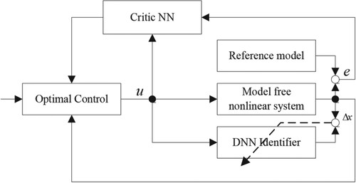
A summary of the ADP-based optimal tracking control algorithm is as follows

• (1) Select the proper initial values of active functions σ(·) and ϕ(·) in Equation (6) and updating gains k₁, k₂, k₃ in Equation (9) for the identifier. σ(·) is usually selected as the sigmoidal function $\sigma (\cdot )=a/\left(1+e^{-bx}\right)-c$ where a, b and c are the designed constants. ψ (·) is selected as ψ (·) =  I. α,β and γ are tuned online according to equations (9). Hence, there is no need to select the initial weight values of α,β and γ. Meanwhile, select the proper function ϕ(·) in Equation (31) and the updating gain μ in Equation (45) for the critic NN ϕ (·) is usually selected as a smooth function consisting of a different combination between state tracking errors.

• (2) The inputs/outputs data of an unknown non-affine nonlinear system (1) is used to train the identifier.

• (3) Adaptive optimal tracking control law consisting of the steady-state control law in an equation and the optimal control law in Equation (32) is obtained based on the first two steps.

5. Simulations

We consider the following two examples to illustrate the theoretical results in this section.

Example

Considering the following non-affine nonlinear system (61) $\begin{array}{rl}\left[\begin{array}{c}{\dot{x}}_1\\ {\dot{x}}_2\end{array}\right]& =\left[\begin{array}{c}-x_1+x_2\\ -0.5x_1-0.5x_2(1-(\cos (2x_1+2{)}^2)\end{array}\right]\\ & +\left[\begin{array}{c}{u}_1\\ \left(\cos \left(2x_1+2\right)\right)+\sin \left(u_2\right)\end{array}\right]\end{array}$(61)

The matrices $Q$ and $R$ of the performance index function are chosen as identify matrices. The control objective is to make the state $x_1$ and $x_2$ follow the desired trajectory $x_{1\text{r}}=\sin t$ and $x_{2r}=\cos \left(t\right)-\sin \left(t\right)$. First, a DNN identifier (6) with the updating law (9) is used to identify the non-affine nonlinear system. Parameters are selected as $k_1=k_2=k_3=1$, active function is selected as $\sigma (\cdot )=2/\left(1+e^{-2x}\right)-0.5$.

The identification error is shown in Figure 2. We can see that the proposed identifier can model the non-affine nonlinear system accurately. Then, with the identified model, the adaptive optimal tracking controller is implemented for the unknown non-affine nonlinear continuous system (61). Define the trajectory error as $e_1=x_1-x_{r1},e_2=x_2-x_{r2}$. The activation function of critic NN is selected as $\varphi =\left[e_1^2,e_1{e}_2,e_2^2\right]$. The adaptive gain of the critic NN is selected as $\mu =100$, and the steady control gain is selected as K = 1200. Figures 3 and 4 represent the trajectory tracking, and the convergence property for the weight of the critic NN is shown in Figure 5, which demonstrates that the proposed adaptive optimal tracking controller can ensure satisfactory tracking performance for an unknown non-affine nonlinear continue system.

Figure 2. State identification error.

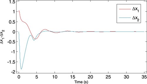
Figure 3. State tracking for x₁.

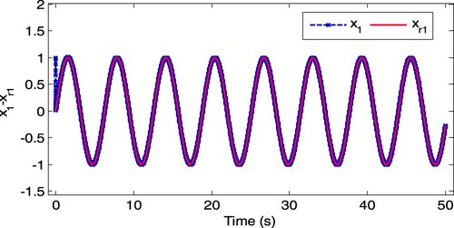
Figure 4. State tracking for x₂.

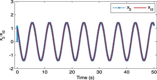
Figure 5. Convergence property for the critic NN weight $x=\left[\text{β}\gamma \right],$.

Example

The classical 2-DOF single-track vehicle model, as shown in Figure 6, is commonly used in AFS/DYC control design [27]. The parameter notations are shown in Table 1.

Figure 6. Single-track vehicle model.

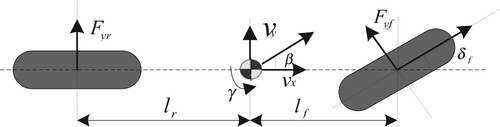
Table 1. Description of vehicle model parameters.

Parameters	Description
M	Vehicle mass
Iz	Yaw inertia
lf,lr	Distance from CG to the front axle and rear axle
Cf0, Cr0	Corner stiffness of the front and rear wheel
Cx	Longitudinal tire stiffness
H	CG height
vx,vy	Vehicle longitudinal and lateral speed
$RMS=\sqrt{\sum _{i=1}^n{e}^2\left(i\right)/n}$	Vehicle longitudinal and lateral acceleration
Fxi, Fyi	Longitudinal and lateral force, i = 1,2,3,4.
Fxwi, Fywi	Longitudinal and lateral tire force
Fzi	The normal force of the ith wheel
g	Gravity acceleration
Rw,Jw	Wheel rolling radius, the moment of inertia
${\omega }_{Wi}$	Wheel angular speed
Twi	Active brake torque
T	Wheel track width
$\mu$	The friction coefficient between tire and road
$\gamma$	Yaw rate about the z-axis
${\alpha }_i,{\sigma }_i$	The ith wheel slip angle, slip ratio
${\delta }_f$	Steer angle of the front wheel

The mathematical model of Figure 6 considering the uncertainty parameters is expressed as follows: (62) $\begin{array}{rl}\dot{x}& =(A+\mathrm{\Delta }A)x+(B+\mathrm{\Delta }B)u+E{\delta }_f\\ y& =Cx\end{array}$(62) where $x=\left[\begin{array}{cc}\text{β}& \gamma \end{array}\right]$ $\text{β}$ is the side slip angel, $\gamma$ is the yaw rate; $u=\left[\begin{array}{c}{\delta }_c\\ M_c\end{array}\right]$, ${\delta }_c$ is the active steer angle, $M_c$ is the corrective yaw moment and ${\delta }_f$ is the driver steer input $\begin{array}{rl}A& =\left[\begin{array}{cc}-2{\displaystyle \frac{C_r+C_f}{m{v}_x}}& -1-2{\displaystyle \frac{C_f{l}_f-C_r{l}_r}{m{v}_x^2}}\\ -2{\displaystyle \frac{C_f{l}_f-C_r{l}_r}{I_z}}& -2{\displaystyle \frac{C_f{l}_f^2+C_r{l}_r^2}{I_z{v}_x}}\end{array}\right],\\ B& =\left[\begin{array}{cc}{\displaystyle \frac{2C_f}{m{v}_x}}& 0\\ {\displaystyle \frac{2C_f{l}_f}{I_z}}& {\displaystyle \frac{1}{I_z}}\end{array}\right],E=\left[\begin{array}{c}{\displaystyle \frac{2C_f}{m{v}_x}}\\ {\displaystyle \frac{2C_f{l}_f}{I_z}}\end{array}\right],\mathrm{\Delta }A=DF{E}_1,\\ \mathrm{\Delta }B& =DF{E}_2,F=\left[\begin{array}{cc}{\rho }_f& 0\\ 0& {\rho }_r\end{array}\right],C=\left[\begin{array}{cc}1& 0\\ 0& 1\end{array}\right]\\ D& =\left[\begin{array}{cc}-{\displaystyle \frac{2C_f{\mathrm{\Delta }}_f}{m{v}_x}}& {\displaystyle \frac{2C_r{\mathrm{\Delta }}_r}{m{v}_x}}\\ -{\displaystyle \frac{2C_f{\mathrm{\Delta }}_f{l}_f}{I_z}}& -{\displaystyle \frac{2C_r{\mathrm{\Delta }}_r{l}_r}{I_z{v}_x}}\end{array}\right],\\ E_1& =\left[\begin{array}{cc}1& {\displaystyle \frac{l_f}{v_x}}\\ -1& {\displaystyle \frac{l_r}{v_x}}\end{array}\right],E_2=\left[\begin{array}{cc}-1& 0\\ 0& 0\end{array}\right].\end{array}$The main object of vehicle stability control is to design the proper controller to make the actual vehicle yaw rate and sideslip to follow the desired responses. The reference model is usually selected as (63) ${\dot{x}}_r=A_r{x}_r+E_r{\delta }_f$(63) where $x_r=\left[\begin{array}{c}{\text{β}}_r\\ {\gamma }_r\end{array}\right],A_r=\left[\begin{array}{cc}-\frac{1}{{\tau }_{\text{β}}}& 0\\ 0& -\frac{1}{{\tau }_r}\end{array}\right]$ $E_r=\left[\begin{array}{c}{\displaystyle \frac{1-\frac{m{l}_f}{2\left(l_f+l_r\right)l_r{C}_r}{v}_x^2}{1+\frac{m}{\left(l_f+l_r\right)}\left(\frac{l_f}{2C_r}-\frac{l_r}{2C_f}\right)v_x^2}}\\ {\displaystyle \frac{\frac{v_x}{l_f+l_r}}{1+\frac{m}{\left(l_f+l_r\right)}\left(\frac{l_f+l_r)}{2C_r}-\frac{l_r}{2C_f}\right)v_x^2}}\end{array}\right]$${\tau }_r,{\tau }_{\text{β}}$ are the designed time constants of raw rate and sideslip angle, respectively.

With the assumption that the variation and uncertainty of tire cornering stiffness can be described as (64) $\{\begin{array}{l}{C}_f=C_{f0}(1+{\mathrm{\Delta }}_f{\rho }_f),||{\rho }_f||\le 1\\ C_r=C_{r0}(1+{\mathrm{\Delta }}_r{\rho }_r),||{\rho }_r||\le 1\end{array}$(64) where $C_{f0},C_{r0}$ and $C_f,C_r$ are the nominal and actual cornering stiffness of the front and rear tires respectively, $C_{f0},C_{r0}$ are the deviation magnitude, ${\rho }_f,{\rho }_r$ are perturbations.

Simulation parameters of the vehicle system are selected as m = 1704kg, C_f= 63224N/rad, C_r= 84680 N/rad, I_z= 3048 kg m², l_f= 1.135 m and l_r= 1.555 m. A 28-degree step steer manoeuvre with an initial speed (of 80 km/h) is simulated to verify the proposed method. The time-varying parameters of C_f and C_r are obtained from (64) by selecting Δ_f, Δ_r as constant 0.5 and ρ_f, ρ_r as band-limited white noise with the amplitude ±0.01. As shown in Figures 7 and 8, the proposed method still demonstrates strong robustness and self-adaptive performance, i.e. less tracking error for yaw rate and sideslip angle, when encountering time-varying cornering stiffness in step steer manoeuvre.

Figure 7. Side-slip angle.

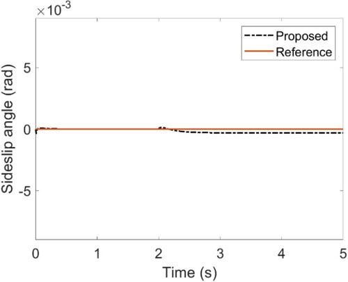
Figure 8. Yaw rate.

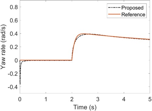
To show the identification performance of the proposed algorithm, the performance index-Root Mean Square (RMS) for the state’s error has been adopted for comparison. (65) $RMS=\sqrt{\sum _{i=1}^n{e}^2\left(i\right)/n}$(65) where n is the number of the simulation steps, $e\left(i\right)$ is the corresponding state response at the ith step.

The RMS values of the side slip angle and yaw rate are 0.915 × 10⁻⁴ and 3.173 × 10⁻⁴, respectively.

6. Conclusions

In this paper, we develop an adaptive optimal controller with a critic-identifier structure to solve the trajectory tracking problem for model uncertain non-affine nonlinear continuous-time system. First, a model-free DNN identifier is designed to reconstruct the unknown dynamic. Then, based on the identification model, an adaptive optimal controller is presented, which can realize the trajectory tracking and stabilize the error dynamic optimally. In addition, a critic NN is introduced to approximate the optimal value function, and a novel robust tuning law is established to update the critic NN weight. The stability of the closed-loop system is proved by the Lyapunov approach. Simulation results of two examples are presented to verify the validity of the proposed approach.

Disclosure statement

No potential conflict of interest was reported by the author(s).

Additional information

Funding

This work is supported by the National Natural Science Foundation of China (NSFC) under Grant 62073298, Key Research and Development Projects of Henan Province in 2022 under Grant 221111240200, Special Application for Key Scientific and Technological Project of Henan Province [Grant Number JDG20220037].

References

- Powell B. Approximate dynamic programming: solving the curses of dimensionality. New Jersey: Wiley-Blackwell; 2007.
- Lebedev D, Margellos K, Goulart P. Convexity and feedback in approximate dynamic programming for delivery time slot pricing. IEEE Trans Control Syst Technol. 2022;30(2):893–900.
- Zhang H, Liu D, Luo Y, et al. Adaptive dynamic programming for control: algorithms and stability. London: Springer; 2013.
- Lewis FL, Liu D, Editors. Approximate dynamic programming and reinforcement learning for feedback control. Hoboken (NJ): Wiley; 2013.
- Werbos P. Approximate dynamic programming for real-time control and neural modeling. handbook of intelligent control, neural, fuzzy, and adaptive approaches. New York (NY): Van Nostrand Reinhold; 1992.
- Miller W, Sutton R, Werbos P. Neural networks for control. Cambridge (MA): MIT Press; 1990.
- Fairbank M, Alonso E, Prokhorov D. Simple and fast calculation of the second-order gradients for globalized dual heuristic dynamic programming in neural networks. IEEE Trans Neural Netw Learn Syst. 2012;23(10):1671–1676.
- Zhu L, Modares H, Peen G, et al. Adaptive suboptimal output-feedback control for linear systems using integral reinforcement learning. IEEE Trans Control Syst Technol. 2015;23(1):264–273.
- Wei Q, Liu D, Shi G. A novel dual iterative q-learning method for optimal battery management in smart residential environments. IEEE Trans Ind Electron. 2015;62(4):2509–2518.
- Bhasin S, Kamalapurkar R, Johnson M, et al. A novel actor-critic-identifier architecture for approximate optimal control of uncertain nonlinear systems. Automatica (Oxf). 2013;49(1):82–92.
- Vrabie D, Pastravanu O, Abu-Khalaf M, et al. Adaptive optimal control for continuous-time linear systems based on policy iteration. Automatica (Oxf). 2009;45:477–484.
- Vamvoudakis K, Lewis F. Online actor critic algorithm to solve the continuous-time infinite horizon optimal control problem. Proc Int Joint Conf Neural Netw. 2009;46:3180–3187.
- Modares H, Lewis F, Naghibi-Sistani M. Adaptive optimal control of unknown constrained-input dystems using policy iteration and neural networks. IEEE Trans Neural Netw Learn Syst. 2013;24(10):1513–1525.
- Na J, Lv Y, Wu X, et al. Approximate optimal tracking control for continuous-time unknown nonlinear systems). Nan Jing, China, Proceedings of the 33rd Chinese control conference; 2014; p. 8990–8995.
- Lv Y, Na J, Yang Q, et al. Online adaptive optimal control for continuous-time nonlinear systems with completely unknown dynamics. Int J Control. 2016;89(1):99–112.
- Zhang H, Cui L, Luo Y. Near-optimal control for nonzero-sum differential games of continuous-time nonlinear systems using single-network ADP. IEEE Trans Cybern. 2013;43(1):2168–2267.
- Wei Q, Liu D. Adaptive dynamic programming for optimal tracking control of unknown nonlinear systems with application to coal gasification. IEEE Trans Autom Sci Eng. 2014;11(4):1020–1036.
- Modares H, Lewis F. Linear quadratic tracking control of partially-unknown continuous-time systems using reinforcement learning. IEEE Trans Autom Control. 2014;59(11):3051–3056.
- Kamalapurkar R, Dinhb H, Bhasin S, et al. Approximate optimal trajectory tracking for continuous-time nonlinear systems. Automatica (Oxf). 2015;51:40–48.
- Lv Y, Ren X, Na J. Adaptive optimal tracking controls of unknown multi-input systems based on nonzero-sum game theory. J Franklin Inst. 2019;22(12):2226–2236.
- Zhang X, Zhang H, Sun Q, et al. Adaptive dynamic programming-based optimal control of unknown nonaffine nonlinear discrete-time systems with proof of convergence. Neurocomputing. 2012;91:48–55.
- Wang H, Tian Y. Non-affine nonlinear systems adaptive optimal trajectory tracking controller design and application. Stud Inf Control. 2015;24(1):5–11.
- Li X, Yu W. Dynamic system identification via recurrent multilayer perceptrons. Inf Sci (Ny). 2002;147:45–63.
- Poznyak A, Yu W, Sanchez E, et al. Nonlinear adaptive trajectory tracking using dynamic neural networks. IEEE Trans Neural Netw. 1999;10(6):1402–1411.
- Abu-Khalaf M, Lewis F. Nearly optimal control laws for nonlinear systems with saturating actuators using a neural network HJB approach. Automatica (Oxf). 2005;41(5):779–791.
- Na J, Yang J, Wu X, et al. Robust adaptive parameter estimation of sinusoidal signals. Automatica (Oxf). 2015;53:376–384.
- Yang X, Wang Z, Peng W. Coordinated control of AFS and DYC for vehicle handling and stability based on optimal guaranteed cost theory. Veh Syst Dyn. 2009;47(1):57–79.