Almost sure stability of Caputo fractional-order switched linear systems with deterministic and stochastic switching signals

Abstract

In this paper, we address the almost sure stability problem of Caputo fractional-order switched linear systems with deterministic and stochastic switching signals (DS-CFLSs). Firstly, due to the non-locality and memory of fractional-order switched systems, an inequality is proposed to solve the difficulties in the discussion of stability. Then, for DS-CFLSs, a deterministic switching strategy is predesigned, and stochastic switching signals are generated by the Markov process. After that, for the globally asymptotic stability almost surely (GAS a.s.) and exponential stability almost surely (ES a.s.) of DS-CFLSs, some sufficient conditions are proposed by using the multi-Lyapunov function and probability analysis methods. Finally, some numerical examples show that our results are effective.

KEYWORDS:

• Caputo fractional-order switched systems
• deterministic switching
• stochastic switching
• multi-Lyapunov functions
• Markov process

1. Introduction

The switched system is a special hybrid system composed of several subsystems and the rules that coordinate the switching between these subsystems. The fractional-order switched system is an extension of the integer-order switched system. Its stability analysis and application are a hot issue in the current research, and are widely used in robot controls [1,2], power electronic systems [3], fault tolerant control [4–10] and the field of fuzzy logic systems [11–13].

At present, the research on fractional-order switched systems mainly focuses on stability problem, such as asymptotic stability and finite-time stability. In [14], the asymptotic stability of a class of continuous-time positive fractional switched systems is studied by using the state-dependent switching and fractional-order co-positive Lyapunov method. The problem that the instantaneous pulse does not need to be consistent with the switching point is solved, and the exponential stability criterion of fractional-order impulsive switched systems is derived by the means of mode-dependent average pulse interval method and the induction method [15]. The sufficient conditions for the asymptotic stability of fractional-order switched systems are given by using the fractional-order Lyapunov function and the minimum dwell-time technique [16]. In [17], the output tracking control problem for a class of fractional-order positive switched system is studied. A new exponential stability criterion is derived by using Lyapunov theory, average dwell-time method and linear matrix inequality. Zhang and Wang [18] discuss the relationship between the stability of integer-order switched systems and fractional-order switched systems, and the problem of robust stabilization of uncertain switched fractional-order switched systems under the common switching law. Feng et al.[19] give the general solution of a class of Caputo fractional differential equations with piece-wise definitions, and on this basis, the finite-time stability of fractional-order switched continuous-time systems is studied. In [20–24], Lyapunov-like functions, multi-Lyapunov functions, co-positive Lyapunov function, average dwell-time switching technique and other methods are used to analyse the finite-time stability and stabilization of fractional-order positive switched, singular switched and uncertain switched systems. According to the different switching mechanisms, these research papers can be divided into fractional-order deterministic switched systems and random switched systems, which are collectively referred to as single-switched systems.

However, facing the increasingly complex control object in practical engineering, in order to accurately describe their internal driving mechanism, some scholars have proposed the dual switching system. The dual switching system is a new type of switching dynamic system that obeys both deterministic switching and stochastic switching. It can be applied to wind power generation systems [25], various complex switching control operations are essential for system stability and optimization [26].

First of all, for integer-order differential equations, the dual switched systems have achieved considerable research results, which mainly focus on the theoretical analysis of stability. In [27], the almost sure stability of a switched Markov jump linear system is studied. Under the conditions of deterministic switching and Markovian switching, two sufficient conditions for exponential almost sure stability are proposed. Then, a condition for almost sure stability of dual switched discrete-time systems is discussed by using the multi-Lyapunov function method and persistent dwell time [28]. Liu et al. [29] proposed that the sign stability of dual switched continuous-time positive systems. In addition, according to the transition probability of Markovian switching, it can be divided into fixed dual switching systems [30] and variable dual switching systems [31,32]. The transition probability of the former is fixed; the latter changes with the switching of the subsystem and is determined by the determination of the switching signal. However, for fractional-order switched systems, the dual switched fractional-order switched system is a relatively new research problem, and the analysis of its related stability problems is still lacking. In addition, due to the special properties of fractional-order switched systems: non-locality and memory. It is controversial whether the initial value of the lower bound of the fractional derivative will be updated with occurrence of switching and whether the fractional integral can be taken directly at the time interval with inconsistent lower bound [33–37], which needs to be further solved. We will propose an inequality in Lemma 3.1 to solve the difficulties in the process of stability proof.

In this paper, we address the almost sure stability problem of Caputo fractional-order switched linear systems with deterministic and stochastic switching signals (DS-CFLSs) by combining with the existing almost sure stability results of integer-order dual switching systems and the unique properties of fractional derivatives. Our main contributions are as follows:

1. Combining DS-CFLSs, a fractional-order dual switching system model is established, and an inequality is proposed to solve the difficulty in the stability proof process.

2. The sufficient conditions of the global asymptotic stability almost surely (GAS a.s.) and exponential stability almost surely (ES a.s.) for the DS-CFLSs are provided based on the multi-Lyapunov function and probability analysis methods.

This article unfolds as follows. In Section 2, we formulate the model and introduce some useful lemmas as well as definitions of system stability. In Section 3, an inequality is proposed and proved, then we present the main criteria that ensure the almost sure stability of DS-CFLSs. We provide some numerical examples to illustrate the feasibility of the established criteria in Section 4. Finally, we close the article with some conclusions in Section 5.

Notations: $\mathbb{R}$ and $\mathbb{N}$, respectively, denote the sets of real numbers and nature numbers. ${\mathbb{R}}^n$ is the set of $n$-dimensional real vectors, $||x||$ represents the Euclidean norm of $x$. Furthermore, $AC$ and $C^1$ represent absolutely continuous and first-order continuous differentiable, respectively.

2. Model formulation and preliminaries

Consider the following DS-CFLSs: (2.1) $\{\begin{array}{l}{}_{t_0}^C{D}_t^{\alpha }x(t)=A_{r(t,\sigma (t))}^{[\sigma (t)]}x(t),t\ge t_0\text{, }\\ x(t_0)=x_0,\end{array}$(2.1) where $\alpha \in (0,1)$; $x(t)\in {\mathbb{R}}^n$ is the state vector; $x_0\in {\mathbb{R}}^n$ is the initial state; $\sigma (t):[t_0,\mathrm{\infty })\to$ $\overline{\mathrm{M}}=\{1,2,\cdots ,M\},M<\mathrm{\infty }$ denotes the deterministic switching signal, which is a right-continuous piece-wise constant function. Let $\sigma (t)=j\in \overline{\mathrm{M}},\mathrm{\forall }t\in [t_k,t_{k+1})$ indicates that the $j$-th Markov subsystem is activated over the interval $[t_k,t_{k+1})$, such as ${}_{t_0}^C{D}_t^{\alpha }x(t)=A_{r(t,j)}^{[j]}x(t)$, where $\{t_k{\}}_{k\in \mathbb{N}}$ represents the $k$-th deterministic switching time instant, and it is assumed that there is no switching at the initial time $t_0=0$. The stochastic switching signal $r(t,\sigma (t)):[t_0,\mathrm{\infty })\times \overline{\mathrm{M}}\to \overline{\mathrm{N}}=\{1,2,\cdots ,N\},N<\mathrm{\infty }$ stands for a right-continuous random piece-wise constant function which is governed by the $N$-mode Markov process. Let $r(t,j)=i\in \overline{\mathrm{N}}$ for $\mathrm{\forall }t\in [{\tau }_v,{\tau }_{v+1})\subset [t_k,t_{k+1})$ indicates that the $i$-th sub-mode is activated over the interval $[{\tau }_v,{\tau }_{v+1})$. That is to say, the active subsystem is ${}_{t_0}^C{D}_t^{\alpha }x(t)=A_i^{[j]}x(t)$ for $\mathrm{\forall }t\in [{\tau }_v,{\tau }_{v+1})\subset [t_k,t_{k+1})$, where ${\tau }_v:[t_k,t_{k+1})\to v\in \{0,1,2,\cdots ,l{\}}_{l<+\mathrm{\infty }}$ is the $v$-th random switching time instant, ${\tau }_0=t_k$, ${\tau }_{l+1}\le t_{k+1}$, $A_i^{[j]}\in {\mathbb{R}}^{n\times n}(j\in \overline{\mathrm{M}},i\in \overline{\mathrm{N}})$ is the system matrix.

Let $(\mathrm{\Omega },\mathrm{\Im },{\{{\mathrm{\Im }}_t\}}_{t\ge 0},\mathrm{P}\text{r})$ be a complete probability space with filtration ${\mathrm{\Im }}_0$ containing all $\mathrm{P}\text{r}$-null sets and ${\mathrm{\Im }}_t$ being monotonically right-continuous. We assume that the deterministic switching signal $\sigma (t)$ is well-defined, i.e. for any $h>0$, there exists a sufficient small real number $\mathrm{\Delta }>0$ such that the deterministic switching signal $\sigma (t)$ is constant over the interval $[h,h+\mathrm{\Delta }]$, that is, $\sigma (t)\equiv j\in \overline{\mathrm{M}}$ for $t\in [h,h+\mathrm{\Delta }]$. Then, for any $j\in \overline{\mathrm{M}}$, the transition probability of the Markov process $r(t,j)$ is defined by (2.2) $\begin{array}{rl}{p}_{zs}^{[j]}(\mathrm{\Delta })& =\mathrm{P}\text{r}\{r(h+\mathrm{\Delta },j)=s|r(h,j)=z)\}\\ & =\{\begin{array}{l}{q}_{zs}^{[j]}\mathrm{\Delta }+o(\mathrm{\Delta }),\text{ z}\ne s,\\ 1+q_{zz}^{[j]}\mathrm{\Delta }+o(\mathrm{\Delta }),\text{ z}=s,\end{array}\end{array}$(2.2) where $z,s\in \overline{\mathrm{N}}$ and $\underset{\mathrm{\Delta }\to 0}{lim}o(\mathrm{\Delta })/\mathrm{\Delta }=0$, $q_{zs}^{[j]}$ is the transition rate from mode $z$ at time $h$ to mode $s$ at time $h+\mathrm{\Delta }$, and satisfy $q_{zs}^{[j]}\ge 0,z\ne s$ and $q_{zz}^{[j]}=-{\sum }_{s=1,s\ne z}^N{q}_{zs}^{[j]}$. Then, the Markov process transition rate matrix ${\mathrm{\Lambda }}^{[j]}$ is given by ${\mathrm{\Lambda }}^{[j]}=[q_{zs}^{[j]}{]}_{N\times N}$. In addition, assume that the Markov process $r(t,\sigma (t))$ is irreducible. Thus, it is ergodic and have a unique invariant distribution ${\mathrm{\Pi }}_{}^{[j]}=[{\pi }_1^{[j]},{\pi }_2^{[j]},\cdots ,{\pi }_N^{[j]}]$, which satisfies ${\mathrm{\Pi }}_{}^{[j]}{\mathrm{\Lambda }}^{[j]}=0,{\sum }_{i=1}^N{\pi }_i^{[j]}=1$.

Let ${\mathrm{T}}_i^{[j]}(t_0,t)$ and ${\mathrm{N}}_i^{[j]}(t_0,t)$ be the accumulated time sojourns and the occurrence number for the subsystem ${}_{t_0}^C{D}_t^{\alpha }x(t)=A_i^{[j]}x(t)$ over the interval $[t_0,t]$, respectively. Then according to the Ergodic theorem ([38], Theorem 3.81) and the strong law of large number in [39], the following statements are obvious:

For arbitrary $t\ge t_0$, $i\in \overline{\mathrm{N}},j\in \overline{\mathrm{M}}$, the random sequence of state dwell-time of Markov process $r(t,\sigma (t))$ satisfies the independent exponential distribution with parameter $e_i^{[j]}$. Then, we can get $\mathrm{P}\text{r}\{\text{li}{\text{m}}_{t\to \mathrm{\infty }}\frac{{\mathrm{T}}_i^{[j]}(t_0,t)}{t-t_0}={\pi }_i^{[j]}\}=1$ and $\mathrm{P}\text{r}\left\{\text{li}{\text{m}}_{t\to \mathrm{\infty }}\frac{{\mathrm{N}}_i^{[j]}(t_0,t)}{t-t_0}={\pi }_i^{[j]}{e}_i^{[j]}\right\}=1$, where we define $e_i^{[j]}=|q_{ii}^{[j]}|$. In addition, for $\mathrm{\forall }{\epsilon }^{\mathrm{\prime }}>0$ is small enough, exist $T({\epsilon }^{\mathrm{\prime }})>0$, when $t\ge T({\epsilon }^{\mathrm{\prime }})$, we have ${\mathrm{T}}_i^{[j]}(t_0,t)\le ({\pi }_i^{[j]}+{\epsilon }^{\mathrm{\prime }})(t-t_0)$ and ${\mathrm{N}}_i^{[j]}(t_0,t)\le ({\pi }_i^{[j]}|q_{ii}^{[j]}|+{\epsilon }^{\mathrm{\prime }})(t-t_0)$.

Based on the above DS-CFLSs (2.1). In this paper, the globally asymptotically stability almost surely (GAS a.s.) and exponentially stable almost surely (ES a.s.) will be studied. The stability is defined in [40], as follows:

1. globally asymptotically stable almost surely (GAS a.s.), if the following two properties are verified simultaneously:

   1. (SP1) for $\mathrm{\forall }\epsilon >0,\mathrm{\exists }\delta (\epsilon )>0,$ such that when $||x_0||<\delta (\epsilon )$, $\mathrm{P}\text{r}({sup}_{t\ge t_0}||x(t)||<\epsilon )=1$;

   2. (SP2) for $\mathrm{\forall }r,\hat{\epsilon }>0,\mathrm{\exists }T(r,\hat{\epsilon })\ge 0,$ such that when $||x_0||<r$, $\mathrm{P}\text{r}\{{sup}_{t\ge T(r,\hat{\epsilon })}||x(t)||<\hat{\epsilon }\}=1$;

2. exponentially stable almost surely (ES a.s.), if for any $t\ge t_0$ and initial condition $x_0\in {\mathbb{R}}^n$, we have $\mathrm{P}\text{r}\left\{{lim}_{t\to \mathrm{\infty }}sup\frac{1}{t-t_0}\ln ||x(t,x_0)||<0\right\}=1.$

Lemma 2.1:

Assume that there exist the continuously differentiable function $x(t):[t_0,\mathrm{\infty })\to {\mathbb{R}}^n$ and positive definite matrices $P_i^{[j]}\in {\mathbb{R}}^n$, then satisfy ${}_{t_0}^C{D}_t^{\alpha }x(t)\in C^1[t_0,\mathrm{\infty }]$ and the quadratic function ${}_{t_0}^C{D}_t^{\alpha }[x^T(t)P_i^{[j]}x(t)]\in C^1[t_0,\mathrm{\infty }]$, which further satisfy the following inequality in [33]: (2.3) $\begin{array}{rl}{}_{t_0}^C{D}_t^{\alpha }[x^T(t)P_i^{[j]}x(t)]& \le [{}_{t_0}^C{D}_t^{\alpha }{x}^T(t)]P_i^{[j]}x(t)\\ & +x^T(t)P_i^{[j]}[{}_{t_0}^C{D}_t^{\alpha }x(t)].\end{array}$(2.3)

Lemma 2.2

[41]

For $\mathrm{\forall }\alpha \in (0,1)$ , $f(t)\in AC[0,\mathrm{\infty }],$ it holds that (2.4) $\begin{array}{rl}{}_{t_0}^C{D}_t^{\alpha }{}_{t_0}^C{D}_t^{\alpha }({}_{t_0}^{}{I}_t^{\alpha }f(t))& =f(t),{}_{t_0}^{}{I}_t^{\alpha }({}_{t_0}^C{D}_t^{\alpha }f(t))\\ & =f(t)-f(t_0).\end{array}$(2.4)

Lemma 2.3

Gronwall-Bellman Inequality [42]

For any two functions $g(t),h(t)\in C^1[a,b]$ . we have $\text{g}(t)\le k+{\int }_a^{t}g(s)h(s)ds$ implies $g(t)\le k\exp ({\int }_a^{t}h(s)ds)$, where $k$ is a positive real number.

Lemma 2.4

$C_p$ Inequality

For $0<a<1$ and arbitrarily $k$ positive real numbers $x_1,x_2,\dots ,x_k$, we have $\sum _{k=1}^n{x}_k^a\le n^{1-a}(\sum _{k=1}^n{x}_k^{}{)}^a$ .

Lemma 2.5

Young’s Inequality

For any two non-negative real numbers $a$ and $b$, we have $ab\le a^p/p+b^q/q$, where $p^{-1}+q^{-1}=1$ and $p,q>0$ .

3. Main results

Firstly, aiming at these controversial problems [33–37], this paper proposes an inequality to solve them. Then, the multi-Lyapunov function method and probability analysis method are used to analyse its stability, and the sufficient conditions for the DS-CFLSs (2.1) to be GAS a.s. and ES a.s. is given.

Lemma 3.1:

For any $\alpha \in (0,1)$ and positive function $f(t)\in AC[t_0,\mathrm{\infty }]$, if there exists a constant $\lambda \in \mathbb{R}$ such that ${}_{t_0}^C{D}_t^{\alpha }f(t)\le \lambda f(t),\mathrm{\forall }t\ge t_0$, then for any two real numbers $a$ and $b$ satisfying $a>b\ge t_0$, we have (3.1) $f(a)-f(b)\le \lambda \frac{1}{\mathrm{\Gamma }(\alpha )}{\int }_b^a{(a-\tau )}^{\alpha -1}f(\tau )d\tau .$(3.1)

Proof:

For any $t\ge t_0$, it follows from ${}_{t_0}^C{D}_t^{\alpha }f(t)\le \lambda f(t)$ and Lemma 2.2, we can get (3.2) $\begin{array}{rl}{}_{{}_{t_0}}^{}{I}_t^{\alpha }[{}_{t_0}^C{D}_t^{\alpha }f(t)]& =f(t)-f(t_0)\\ & =\frac{1}{\mathrm{\Gamma }(\alpha )}{\int }_{t_0}^t{(t-\tau )}^{\alpha -1}[{}_{t_0}^C{D}_t^{\alpha }f(\tau )]d\tau \\ & \le \frac{\lambda }{\mathrm{\Gamma }(\alpha )}{\int }_{t_0}^t{(t-\tau )}^{\alpha -1}f(\tau )d\tau ,\end{array}$(3.2) Then, for arbitrary two real numbers $a$ and $b$ satisfying $a>b\ge t_0$, we obtain (3.3) $\begin{array}{rl}f(b)-f(t_0)& \le \frac{\lambda }{\mathrm{\Gamma }(\alpha )}{\int }_{t_0}^b{(b-\tau )}^{\alpha -1}f(\tau )d\tau [t_0,b),\\ f(a)-f(t_0)& \le \frac{\lambda }{\mathrm{\Gamma }(\alpha )}{\int }_{t_0}^a{(a-\tau )}^{\alpha -1}f(\tau )d\tau [t_0,a),\end{array}$(3.3) Because $0<\alpha <1$, there are $\alpha -1<0$, and $a-\tau >b-\tau >0$ such that $(a-\tau {)}^{\alpha -1}<(b-\tau {)}^{\alpha -1}$. Hence, for any $\tau \in [t_0,b)$, we can infer that (3.4) $\begin{array}{rl}& \frac{1}{\mathrm{\Gamma }(\alpha )}{\int }_{t_0}^b{(b-\tau )}^{\alpha -1}f(\tau )d\tau \\ & >\frac{1}{\mathrm{\Gamma }(\alpha )}{\int }_{t_0}^b{(a-\tau )}^{\alpha -1}f(\tau )d\tau ,\end{array}$(3.4) Case 1: Suppose $\lambda >0$, then it follows from (3.4) that (3.5) $\begin{array}{rl}& \frac{\lambda }{\mathrm{\Gamma }(\alpha )}{\int }_{t_0}^b{(a-\tau )}^{\alpha -1}f(\tau )d\tau \\ & <\frac{\lambda }{\mathrm{\Gamma }(\alpha )}{\int }_{t_0}^b{(b-\tau )}^{\alpha -1}f(\tau )d\tau ,\end{array}$(3.5) Then, (3.6) $\begin{array}{rl}f(a)-f(t_0)& \le \lambda \frac{1}{\mathrm{\Gamma }(\alpha )}{\int }_{t_0}^a{(a-\tau )}^{\alpha -1}f(\tau )d\tau \\ & =\lambda \frac{1}{\mathrm{\Gamma }(\alpha )}{\int }_{t_0}^b{(a-\tau )}^{\alpha -1}f(\tau )d\tau \\ & +\lambda \frac{1}{\mathrm{\Gamma }(\alpha )}{\int }_b^a{(a-\tau )}^{\alpha -1}f(\tau )d\tau \\ & \le \lambda \frac{1}{\mathrm{\Gamma }(\alpha )}{\int }_{t_0}^b{(b-\tau )}^{\alpha -1}f(\tau )d\tau \\ & +\lambda \frac{1}{\mathrm{\Gamma }(\alpha )}{\int }_b^a{(a-\tau )}^{\alpha -1}f(\tau )d\tau \\ & =f(b)-f(t_0)\\ & +\lambda \frac{1}{\mathrm{\Gamma }(\alpha )}{\int }_b^a{(a-\tau )}^{\alpha -1}f(\tau )d\tau ,\end{array}$(3.6) Therefore, (3.7) $f(a)-f(b)\le \lambda \frac{1}{\mathrm{\Gamma }(\alpha )}{\int }_b^a{(a-\tau )}^{\alpha -1}f(\tau )d\tau .$(3.7) Case 2: Assume $\lambda \le 0$, then follow the same process in Case 1 gives (3.7).

Based on the discussion in both Case 1 and Case 2, we have (3.8) $f(a)-f(b)\le \lambda \frac{1}{\mathrm{\Gamma }(\alpha )}{\int }_b^a{(a-\tau )}^{\alpha -1}f(\tau )d\tau ,\text{ (}a>b).$(3.8) This completes the proof.

Remark 3.1:

Due to the lower bound is inconsistent, it is not sure to take directly the fractional integral ${}_{t_k}{I}_t^{\alpha }$ on both sides of the activated subsystem ${}_{t_0}^C{D}_t^{\alpha }x(t)=f_{r(t_k)}(x(t))$ at the dwell-time interval $[t_k,t_{k+1})$. This inequality is provided to solve the above problems.

Now, by using the probability analysis method and the multi-Lyapunov function method, the sufficient conditions for the GAS a. s. and the ES a. s. of the DS-CFLSs (2.1) is given by Theorem 3.2 and Remark 3.3, respectively.

Theorem 3.2:

For any $j\in \overline{\mathrm{M}},i\in \overline{\mathrm{N}}$, suppose that there exist symmetrically positive definite matrices ${\mathrm{P}}_i^{[j]}\in {\mathbb{R}}^{n\times n}$ and the constant ${\lambda }_i^{[j]}\in \mathbb{R}$ and ${\mu }_i^{[j]}>0$, such that the following inequality holds:

(H1) $(A_i^{[j]}{)}^T{\text{P}}_i^{[j]}+{\text{P}}_i^{[j]}{A}_i^{[j]}\le {\lambda }_i^{[j]}{\text{P}}_i^{[j]},\mathrm{\forall }i\in \overline{\mathrm{N}},\mathrm{\forall }j\in \overline{\mathrm{M}},$

(H2) ${\mathrm{P}}_i^{[j]}\le {\mu }_i^{[j]}{\mathrm{P}}_u^{[j]},\mathrm{\forall }i,u\in \overline{\mathrm{N}},i\ne u,\mathrm{\forall }j\in \overline{\mathrm{M}},$

(H3) ${\eta }^{[j]}=({\sum }_{i=1}^N{\pi }_i^{[j]}|q_{ii}^{[j]}|\ln {\mu }_i^{[j]}+\frac{{\lambda }^{\mathrm{\prime }}}{\mathrm{\Gamma }(\alpha +1)}((1-\alpha )\left({\sum }_{i=1}^N{\pi }_i^{[j]}|q_{ii}^{[j]}|\right)+\alpha ))<0,\mathrm{\forall }i\in \overline{\mathrm{N}},\mathrm{\forall }j\in \overline{\mathrm{M}},$

where ${\lambda }^{\mathrm{\prime }}={\sum }_{i=1}^N{\lambda }_i^{[j]}{\pi }_i^{[j]}|q_{ii}^{[j]}|/{\sum }_{i=1}^N{\pi }_i^{[j]}|q_{ii}^{[j]}|$ . Then the DS-CFLSs (2.1) is GAS a.s. under the following switching strategy:

(H4) $\{\begin{array}{l}{t}_0=0\\ \sigma (t_0)=\arg \underset{j\in \overline{\mathrm{M}}}{min}\{\mathrm{E}[x^T(t_0){\mathrm{P}}_{r(t_0,j)}^{[j]}x(t_0)]\}\\ t_1=inf\{t>t_0|\mathrm{E}[x^T(t){\mathrm{P}}_{r(t,\sigma (t_0))}^{[\sigma (t_0)]}x(t)]\\ >\mathrm{E}[x^T(t_0){\mathrm{P}}_{r(t_0,\sigma (t_0))}^{[\sigma (t_0)]}x(t_0)\\ \times \exp \{{\eta }^{[\sigma (t_0)]}\times (t-t_0)\}]\}\\ \sigma (t_1)=\arg \underset{j\in \overline{\mathrm{M}}}{min}\{\mathrm{E}[x^T(t_1){\mathrm{P}}_{r(t_1,j)}^{[j]}x(t_1)]\}\\ ⋮\\ t_k=inf\{t>t_{k-1}|\mathrm{E}[x^T(t){\mathrm{P}}_{r(t,\sigma (t_{k-1}))}^{[\sigma (t_{k-1})]}x(t)]\\ >\mathrm{E}[x^T(t_{k-1}){\mathrm{P}}_{r(t_{k-1},\sigma (t_{k-1}))}^{[\sigma (t_{k-1})]}x(t_{k-1})\\ \times \exp \{{\eta }^{[\sigma (t_{k-1})]}\times (t-t_{k-1})\}]\}\\ \sigma (t_k)=\arg \underset{j\in \overline{\mathrm{M}}}{min}\{\mathrm{E}[x^T(t_k){\mathrm{P}}_{r(t_k,j)}^{[j]}x(t_k)]\}\\ ⋮\end{array}$

where $0=t_0<t_1<\cdots <t_k<\cdots$ and $\{\sigma (t_k)\in \overline{\mathrm{M}}|k\in \mathbb{N}\cup \{0\}\}$ are the switching time sequence and switching index sequence of the deterministic switching signal $\sigma (t)$ over the interval $[t_0,\mathrm{\infty })$, respectively.

Proof.

Define multi-Lyapunov functions as $V_i^{[j]}(x(t),t)=x^T(t){\mathrm{P}}_i^{[j]}x(t),\mathrm{\forall }i\in \overline{\mathrm{N}},j\in \overline{\mathrm{M}}$. When any $t\in [t_k,t_{k+1})$, set $\sigma (t)=\sigma (t_k)\in \overline{\mathrm{M}}$. It should be noted that for $t\in [t_k,t_{k+1})$, the switching is not deterministic, but random. Let $t_k={\tau }_0<{\tau }_1<\cdots <{\tau }_l<t_{k+1}$ be the switching time sequence of the Markov process switching signal $r(t,\sigma (t_k))$ over the interval $[t_k,t_{k+1})$. Then, for $t\in [{\tau }_v,{\tau }_{v+1})\subset [t_k,t_{k+1})$, reset $r(t,\sigma (t_k))=r({\tau }_v,\sigma (t_k))\in \overline{\mathrm{N}}$. Finally, for $\mathrm{\forall }t\in [{\tau }_l,t_{k+1})$, it can be obtained from the condition (H1) and Lemma 2.1: (3.9) $\begin{array}{rl}& {}_{t_0}^C{D}_t^{\alpha }[x^T(t){\mathrm{P}}_{r({\tau }_l,\sigma (t_k))}^{[\sigma (t_k)]}x(t)]\\ & \le {\lambda }_{r({\tau }_l,\sigma (t_k))}^{[\sigma (t_k)]}{x}^T(t){\mathrm{P}}_{r({\tau }_l,\sigma (t_k))}^{[\sigma (t_k)]}x(t),\end{array}$(3.9) Then, according to the inequality of Lemma 3.1, we have (3.10) $\begin{array}{rl}& x^T(t){\mathrm{P}}_{r({\tau }_l,\sigma (t_k))}^{[\sigma (t_k)]}x(t)-x^T({\tau }_l){\mathrm{P}}_{r({\tau }_l,\sigma (t_k))}^{[\sigma (t_k)]}x({\tau }_l)\\ & \le {\lambda }_{r({\tau }_l,\sigma (t_k))}^{[\sigma (t_k)]}\frac{1}{\mathrm{\Gamma }(\alpha )}\\ & \times {\int }_{{\tau }_l}^t{(t-\tau )}^{\alpha -1}{x}^T(\tau ){\mathrm{P}}_{r({\tau }_l,\sigma (t_k))}^{[\sigma (t_k)]}x(\tau )d\tau ,\end{array}$(3.10) By Lemma 2.3 (Gronwall-Bellman Inequality), we obtain (3.11) $\begin{array}{rl}& x^T(t){\mathrm{P}}_{r({\tau }_l,\sigma (t_k))}^{[\sigma (t_k)]}x(t)\\ & \le x^T({\tau }_l){\mathrm{P}}_{r({\tau }_l,\sigma (t_k))}^{[\sigma (t_k)]}x({\tau }_l)\\ & \times \exp \left\{{\lambda }_{r({\tau }_l,\sigma (t_k))}^{[\sigma (t_k)]}\frac{1}{\mathrm{\Gamma }(\alpha )}{\int }_{{\tau }_l}^t{(t-\tau )}^{\alpha -1}d\tau \right\}\\ & \le x^T({\tau }_l){\mathrm{P}}_{r({\tau }_l,\sigma (t_k))}^{[\sigma (t_k)]}x({\tau }_l)\\ & \times \exp \left\{{\lambda }_{r({\tau }_l,\sigma (t_k))}^{[\sigma (t_k)]}\frac{1}{\mathrm{\Gamma }(\alpha +1)}{(t-{\tau }_l)}^{\alpha }\right\},\end{array}$(3.11) Note $[t_k,t_{k+1})=[t_k={\tau }_0,{\tau }_1)\cup [{\tau }_1,{\tau }_2)\cup \cdots \cup [{\tau }_l,{\tau }_{l+1}=t_{k+1})$. After that, separating the time interval, and obtaining the result through the condition (H2): (3.12) $\begin{array}{rl}& x^T(t){\mathrm{P}}_{r({\tau }_l,\sigma (t_k))}^{[\sigma (t_k)]}x(t)\\ & \le x^T({\tau }_l){\mathrm{P}}_{r({\tau }_l,\sigma (t_k))}^{[\sigma (t_k)]}x({\tau }_l)\\ & \times \exp \left\{\frac{{\lambda }_{r({\tau }_l,\sigma (t_k))}^{[\sigma (t_k)]}}{\mathrm{\Gamma }(\alpha +1)}{(t-{\tau }_l)}^{\alpha }\right\}\\ & \le {\mu }_{r({\tau }_l,\sigma (t_k))}^{[\sigma (t_k)]}{x}^T({\tau }_l^{-}){\mathrm{P}}_{r({\tau }_{l-1},\sigma (t_k))}^{[\sigma (t_k)]}x({\tau }_l^{-})\\ & \times \exp \left\{\frac{{\lambda }_{r({\tau }_l,\sigma (t_k))}^{[\sigma (t_k)]}}{\mathrm{\Gamma }(\alpha +1)}{(t-{\tau }_l)}^{\alpha }\right\}\\ & \le {\mu }_{r({\tau }_l,\sigma (t_k))}^{[\sigma (t_k)]}{x}^T({\tau }_{l-1}^{}){\mathrm{P}}_{r({\tau }_{l-1},\sigma (t_k))}^{[\sigma (t_k)]}x({\tau }_{l-1}^{})\\ & \times \exp \{\frac{{\lambda }_{r({\tau }_l,\sigma (t_k))}^{[\sigma (t_k)]}}{\mathrm{\Gamma }(\alpha +1)}{(t-{\tau }_l)}^{\alpha }\\ & \times \frac{{\lambda }_{r({\tau }_{l-1},\sigma (t_k))}^{[\sigma (t_k)]}}{\mathrm{\Gamma }(\alpha +1)}{({\tau }_l-{\tau }_{l-1})}^{\alpha }\}\\ & ⋮\\ & \le {\mu }_{r({\tau }_l,\sigma (t_k))}^{[\sigma (t_k)]}\cdots {\mu }_{r({\tau }_1,\sigma (t_k))}^{[\sigma (t_k)]}{x}^T({\tau }_0^{}){\mathrm{P}}_{r({\tau }_0,\sigma (t_k))}^{[\sigma (t_k)]}x({\tau }_0^{})\\ & \times \exp \left\{\begin{array}{c}{\displaystyle \frac{{\lambda }_{r({\tau }_l,\sigma (t_k))}^{[\sigma (t_k)]}}{\mathrm{\Gamma }(\alpha +1)}}(t-{\tau }_l{)}^{\alpha }+{\displaystyle \frac{{\lambda }_{r({\tau }_{l-1},\sigma (t_k))}^{[\sigma (t_k)]}}{\mathrm{\Gamma }(\alpha +1)}}({\tau }_l-{\tau }_{l-1}{)}^{\alpha }+\cdots +{\displaystyle \frac{{\lambda }_{r({\tau }_0,\sigma (t_k))}^{[\sigma (t_k)]}}{\mathrm{\Gamma }(\alpha +1)}}({\tau }_1-{\tau }_0{)}^{\alpha }\end{array}\right\}\\ & \le \prod _{n=1}^l{\mu }_{r({\tau }_n,\sigma (t_k))}^{[\sigma (t_k)]}{x}^T(t_k){\mathrm{P}}_{r((t_k,\sigma (t_k))}^{[\sigma (t_k)]}x(t_k)\\ & \times \exp \{\frac{{\lambda }_{r({\tau }_l,\sigma (t_k))}^{[\sigma (t_k)]}}{\mathrm{\Gamma }(\alpha +1)}{(t-{\tau }_l)}^{\alpha }\\ & \times {\sum }_{v=0}^{l-1}\frac{{\lambda }_{r({\tau }_v,\sigma (t_k))}^{[\sigma (t_k)]}}{\mathrm{\Gamma }(\alpha +1)}{({\tau }_{v+1}-{\tau }_v)}^{\alpha }\},\end{array}$(3.12) Here, taking ${\lambda }^{\mathrm{\prime }}=\sum _{r({\tau }_v,\sigma (t_k))=1}^N{\lambda }_{r({\tau }_v,\sigma (t_k))}^{[\sigma (t_k)]}{\mathrm{N}}_{r({\tau }_v,\sigma (t_k))}^{[\sigma (t_k)]}(t_k,t)/\sum _{r({\tau }_v,\sigma (t_k))=1}^N{\mathrm{N}}_{r({\tau }_v,\sigma (t_k))}^{[\sigma (t_k)]}(t_k,t)$. According to Lemmas 2.4 2.5 ($C_p$ and Young's Inequality), then for any $t\in [t_k,t_{k+1})$, we can get (3.13) $\begin{array}{rl}& x^T(t){\mathrm{P}}_{r(t,\sigma (t_k))}^{[\sigma (t_k)]}x(t)\\ & \le x^T(t_k){\mathrm{P}}_{r(t_k,\sigma (t_k))}^{[\sigma (t_k)]}x(t_k)\\ & \times \prod _{r({\tau }_v,\sigma (t_k))=1}^N{[{\mu }_{r({\tau }_v,\sigma (t_k))}^{[\sigma (t_k)]}]}^{{\mathrm{N}}_{r({\tau }_v,\sigma (t_k))}^{[\sigma (t_k)]}(t_k,t)}\\ & \times \exp \{\frac{{\lambda }^{\mathrm{\prime }}}{\mathrm{\Gamma }(\alpha +1)}[{(t-{\tau }_l)}^{\alpha }\\ & +{\sum }_{v=0}^{l-1}{({\tau }_{v+1}-{\tau }_v)}^{\alpha }]\}\\ & \le x^T(t_k){\mathrm{P}}_{r(t_k,\sigma (t_k))}^{[\sigma (t_k)]}x(t_k)\\ & \times \exp \{{\sum }_{r({\tau }_v,\sigma (t_k))=1}^N{\mathrm{N}}_{r({\tau }_v,\sigma (t_k))}^{[\sigma (t_k)]}(t_k,t)\\ & \times \ln {\mu }_{r({\tau }_v,\sigma (t_k))}^{[\sigma (t_k)]}\}\\ & \times \exp \{\frac{{\lambda }^{\mathrm{\prime }}}{\mathrm{\Gamma }(\alpha +1)}({\sum }_{r({\tau }_v,\sigma (t_k))=1}^N\\ & \times {{\mathrm{N}}_{r({\tau }_v,\sigma (t_k))}^{[\sigma (t_k)]}(t_k,t)+1)}^{1-\alpha }{(t-t_k)}^{\alpha }\}\\ & \le x^T(t_k){\mathrm{P}}_{r(t_k,\sigma (t_k))}^{[\sigma (t_k)]}x(t_k)\\ & \times \exp \{{\sum }_{r({\tau }_v,\sigma (t_k))=1}^N{\mathrm{N}}_{r({\tau }_v,\sigma (t_k))}^{[\sigma (t_k)]}(t_k,t)\\ & \times \ln {\mu }_{r({\tau }_v,\sigma (t_k))}^{[\sigma (t_k)]}\}\\ & \times \exp \{\frac{{\lambda }^{\mathrm{\prime }}}{\mathrm{\Gamma }(\alpha +1)}[(1-\alpha )({\sum }_{r({\tau }_v,\sigma (t_k))=1}^N\\ & \times {\mathrm{N}}_{r({\tau }_v,\sigma (t_k))}^{[\sigma (t_k)]}(t_k,t)+1)+\alpha (t-t_k)]\},\end{array}$(3.13) Then by ${\mathrm{N}}_{r({\tau }_v,\sigma (t_k))}^{[\sigma (t_k)]}(t_k,t)\le ({\pi }_{r({\tau }_v,\sigma (t_k))}^{[\sigma (t_k)]}|q_{r({\tau }_v,\sigma (t_k)),r({\tau }_v,\sigma (t_k))}^{[\sigma (t_k)]}|+{\epsilon }^{\mathrm{\prime }})(t-t_k\text{) a}\text{.s}\text{.}$, we can obtain (3.14) $\begin{array}{rl}{x}^T(t){\mathrm{P}}_{r(t,\sigma (t_k))}^{[\sigma (t_k)]}x(t)& \le x^T(t_k){\mathrm{P}}_{r(t_k,\sigma (t_k))}^{[\sigma (t_k)]}x(t_k)m\\ & \times \exp \{{\eta }^{[\sigma (t_k)]}\times (t-t_k)\}\text{ a}\text{.s}\text{. ,}\end{array}$(3.14) where $m=\exp \{{\lambda }^{\mathrm{\prime }}(1-\alpha )/\mathrm{\Gamma }(\alpha +1)\}$, $\begin{array}{rl}{\lambda }^{\mathrm{\prime }}& =\sum _{r({\tau }_v,\sigma (t_k))=1}^N\\ & [{\lambda }_{r({\tau }_v,\sigma (t_k))}^{[\sigma (t_k)]}({\pi }_{r({\tau }_v,\sigma (t_k))}^{[\sigma (t_k)]}|q_{r({\tau }_v,\sigma (t_k)),r({\tau }_v,\sigma (t_k))}^{[\sigma (t_k)]}|+{\epsilon }^{\mathrm{\prime }})]\\ & /\sum _{r({\tau }_v,\sigma (t_k))=1}^N({\pi }_{r({\tau }_v,\sigma (t_k))}^{[\sigma (t_k)]}|q_{r({\tau }_v,\sigma (t_k)),r({\tau }_v,\sigma (t_k))}^{[\sigma (t_k)]}|+{\epsilon }^{\mathrm{\prime }}),\end{array}$ $\begin{array}{r}{\eta }^{[\sigma (t_k)]}=\left(\begin{array}{c}{\displaystyle \sum _{r({\tau }_v,\sigma (t_k))=1}^N({\pi }_{r({\tau }_v,\sigma (t_k))}^{[\sigma (t_k)]}|q_{r({\tau }_v,\sigma (t_k)),r({\tau }_v,\sigma (t_k))}^{[\sigma (t_k)]}|+\epsilon )\ln {\mu }_{r({\tau }_v,\sigma (t_k))}^{[\sigma (t_k)]}+{\displaystyle \frac{{\lambda }^{\mathrm{\prime }}}{\mathrm{\Gamma }(\alpha +1)}}((1-\alpha )({\displaystyle \sum _{r({\tau }_v,\sigma (t_k))=1}^N({\pi }_{r({\tau }_v,\sigma (t_k))}^{[\sigma (t_k)]}}|q_{r({\tau }_v,\sigma (t_k)),r({\tau }_v,\sigma (t_k))}^{[\sigma (t_k)]}|+{\epsilon }^{\mathrm{\prime }})\phantom{{\displaystyle \sum _{r({\tau }_v,\sigma (t_k))=1}^N}})+\alpha )}\end{array}\right).\end{array}$

Now, for any $t\in [t_0,\mathrm{\infty })$, designing a switching sequence $\{(t_0,\sigma (t_0)),(t_1,\sigma (t_1)),\cdots ,(t_k,\sigma (t_k)),\cdots \}$ to deterministic the switching signal $\sigma (t)$, which has been given in the condition (H4). Then, according to the switching strategy, it can be obtained from Equation (3.14): (3.15) $\begin{array}{rl}& \mathrm{E}[x^T(t){\mathrm{P}}_{r(t,\sigma (t_k))}^{[\sigma (t_k)]}x(t)]\\ & \le \mathrm{E}[x^T(t_k){\mathrm{P}}_{r(t_k,\sigma (t_k))}^{[\sigma (t_k)]}x(t_k)]\\ & \times m\exp \{{\eta }^{[\sigma (t_k)]}\times (t-t_k)\}\\ & \le \mathrm{E}[x^T(t_k^{-}){\mathrm{P}}_{r(t_{k-1},\sigma (t_{k-1}))}^{[\sigma (t_{k-1})]}x(t_k^{-})]\\ & \times m\exp \{{\eta }^{[\sigma (t_k)]}\times (t-t_k)\}\\ & \le \mathrm{E}[x^T(t_{k-1}^{}){\mathrm{P}}_{r(t_{k-1},\sigma (t_{k-1}))}^{[\sigma (t_{k-1})]}x(t_{k-1}^{})]\\ & \times m\exp \{{\eta }^{[\sigma (t_k)]}\times (t-t_k)+{\eta }^{[\sigma (t_{k-1})]}\\ & \times (t_k-t_{k-1})\}\\ & ⋮\\ & \le \mathrm{E}[x^T(t_0){\mathrm{P}}_{r(t_0,\sigma (t_0))}^{[\sigma (t_0)]}x(t_0)]\\ & \times m\exp \left\{\begin{array}{c}{\eta }^{[\sigma (t_k)]}\times (t-t_k)+{\eta }^{[\sigma (t_{k-1})]}\\ \times (t_k-t_{k-1})\\ +\cdots +{\eta }^{[\sigma (t_0)]}\times (t_1-t_0)\end{array}\right\},\end{array}$(3.15) Hence, set ${\eta }^{\mathrm{\prime }}\text{ = ma}{\text{x}}_{j\in \overline{\mathrm{M}}}\{{\eta }^{[j]}\}$, (3.16) $\begin{array}{rl}\mathrm{E}[x^T(t){\mathrm{P}}_{r(t,\sigma (t_k))}^{[\sigma (t_k)]}x(t)]& \le \mathrm{E}[x^T(t_0){\mathrm{P}}_{r(t_0,\sigma (t_0))}^{[\sigma (t_0)]}x(t_0)]\\ & \times m\exp \{{\eta }^{\mathrm{\prime }}\times (t-t_0)\},\end{array}$(3.16) Then, we can know ${\eta }^{\mathrm{\prime }}<0$ from the condition (H3), so ${\int }_{t_0}^{\mathrm{\infty }}\mathrm{E}[x^T(t){\mathrm{P}}_{r(t,\sigma (t))}^{[\sigma (t)]}x(t)]dt<\mathrm{\infty }$. Through Tonelli's theorem, we get (3.17) $\begin{array}{rl}& {\int }_{t_0}^{\mathrm{\infty }}\mathrm{E}[x^T(t){\mathrm{P}}_{r(t,\sigma (t))}^{[\sigma (t)]}x(t)]dt\\ & =\mathrm{E}\left[{\int }_{t_0}^{\mathrm{\infty }}{x}^T(t){\mathrm{P}}_{r(t,\sigma (t))}^{[\sigma (t)]}x(t)dt\right]<\mathrm{\infty },\end{array}$(3.17) For any $x(t)\in {\mathbb{R}}^n$, $i\in \overline{\mathrm{N}},j\in \overline{\mathrm{M}}$, we have (3.18) ${\zeta }_i^{[j]}||x(t)|{|}^2\le x^T(t){\mathrm{P}}_i^{[j]}x(t)\le {\beta }_i^{[j]}||x(t)|{|}^2,$(3.18) where ${\zeta }_i^{[j]}={\lambda }_{min}({\mathrm{P}}_i^{[j]})\in {\kappa }_{\mathrm{\infty }}$, ${\beta }_i^{[j]}={\lambda }_{max}({\mathrm{P}}_i^{[j]})\in {\kappa }_{\mathrm{\infty }}$, ${\lambda }_{min}(\cdot )$ and ${\lambda }_{max}(\cdot )$ represent the minimum eigenvalue and the maximum eigenvalue, respectively. By (3.17), ${\int }_{t_0}^{\mathrm{\infty }}{min}_{i\in \overline{\mathrm{N}},j\in \overline{\mathrm{M}}}\{{\zeta }_i^{[j]}\}{||x(t)||}^{2}dt<\mathrm{\infty }$, then from Lemma 7 in [40], we can get $\text{li}{\text{m}}_{t\to \mathrm{\infty }}||x(t)||=0\text{ a}\text{.s}\text{.}$. So, for two arbitrary positive numbers $r,\hat{\epsilon }>0$, there exists $T(r,\hat{\epsilon })\ge 0$, when $||x_0||<r$, so that $\text{su}{\text{p}}_{t\ge T(r,\hat{\epsilon })}||x(t)||<\hat{\epsilon }\text{ a}\text{.s}\text{.}$. The property SP2) in the definition of stability is proved. In addition, it is obvious that any $t\ge t_0$, (3.19) $\begin{array}{rl}\underset{i\in \overline{\mathrm{N}},j\in \overline{\mathrm{M}}}{min}\{{\zeta }_i^{[j]}\}||x(t)|{|}^2& \le \mathrm{E}[x^T(t){\mathrm{P}}_{r(t,\sigma (t))}^{[\sigma (t)]}x(t)]\\ & \le \mathrm{E}[x^T(t_0){\mathrm{P}}_{r(t_0,\sigma (t_0))}^{[\sigma (t_0)]}x(t_0)]\\ & \times m\exp \{{\eta }^{\mathrm{\prime }}\times (t-t_0)\}\\ & \le \underset{i\in \overline{\mathrm{N}},j\in \overline{\mathrm{M}}}{max}\{{\beta }_i^{[j]}\}||x(t_0)|{|}^2\\ & \times m\exp \{{\eta }^{\mathrm{\prime }}\times (t-t_0)\},\end{array}$(3.19) Through ${\eta }^{\mathrm{\prime }}<0$, we know that (3.20) $\text{su}{\text{p}}_{t\ge t_0}\left(\gamma ||x_0||\sqrt{m}\exp \left\{\frac{1}{2}{\eta }^{\mathrm{\prime }}\times (t-t_0)\right\}\right)<\mathrm{\infty }\text{ a}\text{.s}\text{.,}$(3.20) where $\gamma =\sqrt{{max}_{i\in \overline{\mathrm{N}},j\in \overline{\mathrm{M}}}\{{\beta }_i^{[j]}\}/{min}_{i\in \overline{\mathrm{N}},j\in \overline{\mathrm{M}}}\{{\zeta }_i^{[j]}\}}$.

Therefore, for an arbitrary positive number $\epsilon >0$, there is an arbitrary $\delta (\epsilon )>0$ and small enough, when $||x_0||<\delta (\epsilon )$, so that $\text{su}{\text{p}}_{t\ge t_0}||x(t)||<\epsilon \text{ a}\text{.s}\text{.}$. The property SP1) in the definition of stability is also proved. So, the DS-CFLSs (2.1) is GAS a.s. under the conditions (H1)–(H3) and the switching rule of (H4), and the proof is completed.

Remark 3.3:

According to (3.19), arbitrary $t\ge t_0$, we obtain $||x(t)||\le \gamma ||x_0||\sqrt{m}\exp \left\{\frac{1}{2}{\eta }^{\mathrm{\prime }}\times (t-t_0)\right\}\text{ a}\text{.s}\text{.}$, It is not difficult to figure out by calculation $\underset{t\to \mathrm{\infty }}{lim}\frac{1}{t-t_0}\ln ||x(t)||\le \frac{1}{2}{\eta }^{\mathrm{\prime }}<0\text{ a}\text{.s}\text{.}$ Hence, the DS-CFLSs (2.1) is ES a.s. under the conditions (H1)–(H3) and the switching rule of (H4).

4. Numerical example

In this section, two examples are given to reveal the effectiveness of the main results in Section 3.

Example 1:

Consider the DS-CFLSs (2.1), with $N=M=2$ and (4.1) $\begin{array}{rl}{A}_1^{[1]}& =\left[\begin{array}{cc}-2& 0\\ 1& -1\end{array}\right],A_2^{[1]}=\left[\begin{array}{cc}-3& 1\\ 2& -3\end{array}\right],\\ A_1^{[2]}& =\left[\begin{array}{cc}-1& 0\\ 0& -1\end{array}\right],A_2^{[2]}=\left[\begin{array}{cc}-2& 1\\ 1& -2\end{array}\right],\\ x_0& ={\left[\begin{array}{cc}1& -1\end{array}\right]}^T.\end{array}$(4.1) Selecting, $\alpha =0.7,{\epsilon }^{\mathrm{\prime }}=1,{\lambda }_1^{[1]}=-2,{\lambda }_2^{[1]}=2,{\lambda }_1^{[2]}=1,{\lambda }_2^{[2]}=-3$, ${\mu }_1^{[1]}=2,{\mu }_2^{[1]}=1.2,{\mu }_1^{[2]}=0.8,{\mu }_2^{[2]}=1.5$. The transition rate matrices of the Markov process switching signals $r(t,1)$ and $r(t,\text{2})$ are ${\mathrm{\Lambda }}_{}^{[1]}=\left[\begin{array}{cc}-2& 2\\ 1& -1\end{array}\right]$ and ${\mathrm{\Lambda }}_{}^{[2]}=\left[\begin{array}{cc}-1& 1\\ 3& -3\end{array}\right]$, respectively.

In addition, its stationary distribution is ${\mathrm{\Pi }}_{}^{[1]}=[\begin{array}{cc}2/3& 1/3\end{array}]$ and ${\mathrm{\Pi }}_{}^{[2]}=[\begin{array}{cc}1/4& 3/4\end{array}]$. Therefore, it can be verified: (4.2) $\begin{array}{rl}{\eta }^{[1]}& =\left(\begin{array}{c}{\displaystyle \sum _{i=1}^N({\pi }_i^{[1]}|q_{ii}^{[1]}|+{\epsilon }^{\mathrm{\prime }})\ln {\mu }_i^{[1]}+{\displaystyle \frac{{\lambda }^{\mathrm{\prime }}}{\mathrm{\Gamma }(\alpha +1)}}\left((1-\alpha )\left({\displaystyle \sum _{i=1}^N({\pi }_i^{[1]}|q_{ii}^{[1]}|+{\epsilon }^{\mathrm{\prime }})}\right)+\alpha \right)}\end{array}\right)\\ & =-0.7798<0,\\ {\eta }^{[2]}& =\left(\begin{array}{c}{\displaystyle \sum _{i=1}^N({\pi }_i^{[2]}|q_{ii}^{[2]}|+{\epsilon }^{\mathrm{\prime }})\ln {\mu }_i^{[2]}+{\displaystyle \frac{{\lambda }^{\mathrm{\prime }}}{\mathrm{\Gamma }(\alpha +1)}}\left((1-\alpha )\left({\displaystyle \sum _{i=1}^N({\pi }_i^{[2]}|q_{ii}^{[2]}|+{\epsilon }^{\mathrm{\prime }})}\right)+\alpha \right)}\end{array}\right)\\ & =-3.2229<0,\end{array}$(4.2) Then, by (H1) and (H2), we can solve the matrices ${\mathrm{P}}_i^{[j]}(i=1,2;j=1,2)$, (4.3) $\begin{array}{rl}{\mathrm{P}}_1^{[1]}& =\left[\begin{array}{cc}5.5505& 2.2324\\ 2.2324& 2.2324\end{array}\right],\\ {\mathrm{P}}_2^{[1]}& =\left[\begin{array}{cc}0.2667& -0.2549\\ -0.2549& 0.2469\end{array}\right],\\ {\mathrm{P}}_1^{[2]}& =\left[\begin{array}{cc}0.4680& 0\\ 0& 0.4680\end{array}\right],{\mathrm{P}}_2^{[2]}=\left[\begin{array}{cc}3.9065& 0\\ 0& 3.9065\end{array}\right].\end{array}$(4.3) Figures 1 and 2 show the deterministic switching signal and the state trajectory of $x(t)$ for the switching system (2.1), respectively.

Figure 1. Deterministic switching signal $\sigma (t)$.

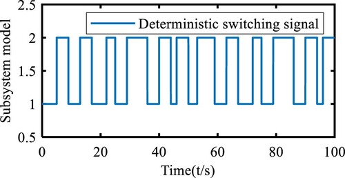
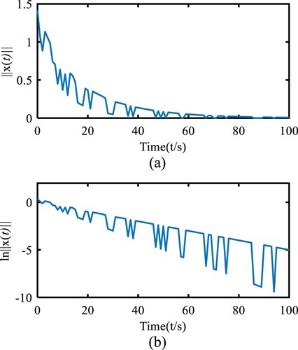
Figure 2. The state trajectory of $x(t)$: (a) the trajectory of $||x(t)||$ and (b) the trajectory of $\ln ||x(t)||$.

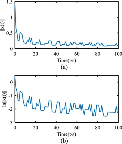
From Figure 2(a and b), we can see that the DS-CFLSs (2.1) is GAS a.s. and ES a.s. under the sufficient conditions (H1)–(H3) and the switching strategy of (H4) (the deterministic switching signal of Figure 1), respectively.

Example 2:

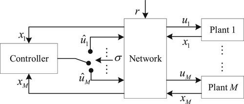
Next, we will illustrate the application of fractional-order dual switching system through the scheduling problem of a multi-loop network control system (NCS) with packet loss in [43]. Suppose that $M$ linear plants must be controlled by a single regulator, and the input–output data are switched through a shared network, as shown in Figure 3. The scheduling signal $\sigma (t)$ determines that the regulator is allowed to control only one plant at a time. The transmission of sensor/actuator data over the network is affected by random faults generated by Markov processes $r(t,\sigma (t))$. For simplicity, it is assumed that each sensor can transmit complete state information without failure, so the regulator has full access to state information from all plants. In addition, the effect of interference is ignored here. For the regulator-actuator channel, let $r(t,\sigma (t))=1$ represents the fail-free mode when all packets are transmitted correctly. If no packet is sent, set $r(t,\sigma (t))=2$ to exit the packet mode. Assume that the stability and performance requirements can then be met by designing a scheduling signal $\sigma (t)$ (a deterministic switching strategy).

Figure 3. The multi-loop NCS.

Consider a fractional-order dual switching NCS with $M=2$, described as (4.4) ${}_{t_0}^C{D}_t^{\alpha }{x}_j(t)=F_j{x}_j(t)+G_j{u}_j(t),j=1,2.$(4.4) Let the state feedback control law be (4.5) ${\hat{u}}_j(t)=\{\begin{array}{ll}{K}_j{x}_j(t),& \text{ if }\sigma (t\text{) = }j\\ 0,& \text{ if }\sigma (t)\ne j\end{array}$(4.5) The real actuator signal affected by random packet loss is (4.6) $u_j(t)=\{\begin{array}{ll}{\hat{u}}_j(t),& \text{ if }r(t,\sigma (t))=i=1\\ 0,& \text{ if }r(t,\sigma (t))=i=2\end{array}$(4.6) Let $x(t)=[x_1(t)x_2(t){]}^T$. Then, by means of (4.5) and (4.6), the expression (4.4) can be rewritten as (4.7) ${}_{t_0}^C{D}_t^{\alpha }x(t)=A_i^{[j]}x(t),i=j=1,2.$(4.7) where $A_1^1=\left[\begin{array}{cc}{F}_1+G_1{K}_1& 0\\ 0& F_2\end{array}\right]$, $A_1^2=\left[\begin{array}{cc}{F}_1& 0\\ 0& F_2+G_2{K}_2\end{array}\right]$, $A_2^1=A_2^2=\left[\begin{array}{cc}{F}_1& 0\\ 0& F_2\end{array}\right]$.

Assuming $F_1=-0.1,F_2=-0.2$, $G_1=G_2=1$ and the controller gains are $K_1=K_2=-1$. Then, selecting $\alpha =0.7,$ ${\epsilon }^{\mathrm{\prime }}=1,$ ${\lambda }_1^{[1]}=-2,{\lambda }_2^{[1]}=1,{\lambda }_1^{[2]}=2,{\lambda }_2^{[2]}=-4$, ${\mu }_1^{[1]}=1,$. ${\mu }_2^{[1]}=2,{\mu }_1^{[2]}=2,{\mu }_2^{[2]}=3$ and $x_0={\left[\begin{array}{cc}1& -1\end{array}\right]}^T.$ The transition rate matrices of theMarkov process switching signals $r(t,1)$ and $r(t,\text{2})$ are ${\mathrm{\Lambda }}_{}^{[1]}=[-5,5;10,-10]$ and ${\mathrm{\Lambda }}_{}^{[2]}=[-8,8;4,-4]$, respectively. In addition, its stationary distribution is ${\mathrm{\Pi }}_{}^{[1]}=[\begin{array}{cc}2/3& 1/3\end{array}]$ and ${\mathrm{\Pi }}_{}^{[2]}=[\begin{array}{cc}1/2& 1/2\end{array}]$. Therefore, it can be verified: (4.8) ${\eta }^{[1]}==-0.5339<0,{\eta }^{[2]}==-0.7506<0,$(4.8) Then, by (H1) and (H2), we can solve the matrices ${\mathrm{P}}_i^{[j]}(i=1,2;j=1,2)$, (4.9) $\begin{array}{rl}{\mathrm{P}}_1^{[1]}& =\left[\begin{array}{cc}2.1532& 0\\ 0& -0.000\end{array}\right],\\ {\mathrm{P}}_2^{[1]}& =\left[\begin{array}{cc}0.3886& 0\\ 0& -0.1749\end{array}\right],\\ {\mathrm{P}}_1^{[2]}& =\left[\begin{array}{cc}1.5287& 0\\ 0& 1.5287\end{array}\right],{\mathrm{P}}_2^{[2]}=\left[\begin{array}{cc}9.7862& 0\\ 0& 9.7862\end{array}\right].\end{array}$(4.9) Figures 4 and 5 show the deterministic switching signal and the state trajectory of $x(t)$ for the switching system (4.4), respectively.

Figure 4. Deterministic switching signal $\sigma (t)$.

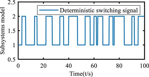
Figure 5. The state trajectory of $x(t)$: (a) the trajectory of $||x(t)||$ and (b) the trajectory of $\ln ||x(t)||$.

In the same way, from Figure 5(a and b), it can be seen that the state of the fractional-order dual switching NCS gradually converges, then the system is GAS a.s and ES a.s.

5. Conclusions

This paper mainly studies the almost sure stability problem of the DS-CFLSs. The sufficient conditions of the global asymptotic stability almost surely (GAS a.s.) and exponential stability almost surely (ES a.s.) for the DS-CFLSs are given by using the multi-Lyapunov function and probability analysis methods. Finally, some numerical examples are provided to demonstrate the validity of the results. Furthermore, we will further discuss the stability of DS-CFLSs with control, disturbance and variable-order.

Disclosure statement

No potential conflict of interest was reported by the author(s).

Additional information

Funding

This research was supported by the National Natural Science Foundation of China [grant number 61813006], [grant number 61973329]; the Key Projects of Basic Research Program of Guizhou Province [grant number 20191416]; the Innovation Group of Guizhou Education Department [grant number Qianjiaohe KY [2021]012]; the Science and Technology Fund of Guizhou Province [grant number Qiankehe [2020]1Y266]; the innovation team of University in Guozhou Province [grant number 2022033].

References

- Gong WL, Xiao J, Han S, et al. Research on robot wireless charging system based on constant-voltage and constant-current mode switching. Energy Rep. 2022;8(4):940–948. doi:10.1016/j.egyr.2022.02.025
- Zhang XL, Huang Y, Wang ST, et al. Hierarchical autonomous switching control of a multi-modes omnidirectional mobile robot. Mechatronics. 2021;80:102692. doi:10.1016/j.mechatronics.2021.102692
- Qu L, Yu ZQ, Zeng R, et al. Parallel breaking characteristics of diode-bridge power electronic switch for DC circuit breaker. Int J Electr Power Energy Syst. 2022;138:107929. doi:10.1016/j.ijepes.2021.107929
- Himanshukumar RP, Vipul AS. A metaheuristic approach for interval type-2 fuzzy fractional order fault-tolerant controller for a class of uncertain nonlinear system. Automatika. 2022;63(4):656–675. doi:10.1080/00051144.2022.2061818
- Himanshukumar RP, Vipul AS. Type-2 fuzzy logic applications designed for active parameter adaptation in metaheuristic algorithm for fuzzy fault-tolerant controller. Int J Intell Comput Cybern. 2023;16(2):198–222. doi:10.1108/IJICC-01-2022-0011
- Himanshukumar RP. Fuzzy-based metaheuristic algorithm for optimization of fuzzy controller: fault-tolerant control application. Int J Intell Comput Cybern. 2022;15(4):599–624. doi:10.1108/IJICC-09-2021-0204
- Raval S, Himanshukumar RP, Vipul AS. Neural network-based control framework for SISO uncertain system: passive fault tolerant approach. INFUS 2020: Intelligent and Fuzzy Techniques: Smart and Innovative Solutions, AISC 1197; 2021. p. 1039–1047.
- Himanshukumar RP, Vipul AS. Stable fault tolerant controller design for Takagi-Sugeno fuzzy model-based control systems via linear matrix inequalities: three conical tank case study. Energies. 2019;12:2221. doi:10.3390/en12112221
- Himanshukumar RP, Vipul AS. Shadowed Type-2 fuzzy sets in dynamic parameter adaption in cuckoo search and flower pollination algorithms for optimal design of fuzzy fault-tolerant controllers. Math Comput Appl. 2022;27:89.
- Raval S, Himanshukumar RP, Vipul AS. Fault tolerant controller comparative study and analysis for benchmark two tank interacting level control system. SN Computer Science. 2021;2:93. doi:10.1007/s42979-021-00489-9
- Himanshukumar RP, Vipul AS. Stable fuzzy controllers via LMI approach for non-linear systems described by type-2 T–S fuzzy model. Int J Intell Comput Cybern. 2021;14(3):509–531. doi:10.1108/IJICC-02-2021-0024
- Himanshukumar RP, Raval SK, Vipul AS. A novel design of optimal intelligent fuzzy TID controller employing GA for nonlinear level control problem subject to actuator and system component fault. Int J Intell Comput Cybern. 2021;14(1):17–32. doi:10.1108/IJICC-11-2020-0174
- Himanshukumar RP, Vipul AS. A fractional and integer order PID controller for nonlinear system: two non-interacting conical tank process case study. Advances in control systems and its infrastructure. Lect Notes Electr Eng. 2020;604:37–55. doi:10.1007/978-981-15-0226-2_4
- Zhao XD, Yin YF, Zheng XL. State-dependent switching control of switched positive fractional-order systems. ISA Trans. 2016;62:103–108. doi:10.1016/j.isatra.2016.01.011
- Zhan T, Ma S, Li W, et al. Exponential stability of fractional-order switched systems with mode-dependent impulses and its application. IEEE Trans Cybern. 2022;52(11):11516–11525.
- Yang Y, Chen G. Stability of a class of fractional order switched systems, IEEE Advanced Information Technology. Electronic and Automation Control Conference (IAEAC); 2015. p. 87–90.
- Sakthivel R, Mohanapriya S, Ahn CK, et al. Output tracking control for fractional-order positive switched systems with input time delay. IEEE Trans Circuits Syst Express Briefs. 2019;66(6):1013–1017. doi:10.1109/TCSII.2018.2871034
- Zhang XF, Wang Z. Stability and robust stabilization of uncertain switched fractional order systems. ISA Trans. 2020;103:1–9. doi:10.1016/j.isatra.2020.03.019
- Feng T, Guo LH, Wu BW, et al. Stability analysis of switched fractional-order continuous-time systems. Nonlinear Dyn. 2020;102:2467–2478. doi:10.1007/s11071-020-06074-8
- Mai VT, Dinh CH. Robust finite-time stability and stabilization of a class of fractional-order switched nonlinear systems. J Syst Sci Complex. 2019;32:1479–1497. doi:10.1007/s11424-019-7394-y
- Feng T, Wu B, Liu L, et al. Finite-time stability and stabilization of fractional-order switched singular continuous-time systems. Circuits Syst Signal Process. 2019;38:5528–5548. doi:10.1007/s00034-019-01159-1
- Liang J, Wu B, Wang Y, et al. Input–output finite-time stability of fractional-order positive switched systems. Circuits Syst Signal Process. 2019;38:1619–1638. doi:10.1007/s00034-018-0942-1
- Zhang J, Zhao X, Chen Y. Finite-time stability and stabilization of fractional order positive switched systems. Circuits Syst Signal Process. 2016;35:2450–2470. doi:10.1007/s00034-015-0236-9
- Liu L, Cao X, Fu Z, et al. Finite-time control of uncertain fractional-order positive impulsive switched systems with mode-dependent average dwell time. Circuits Syst Signal Process. 2018;37:3739–3755. doi:10.1007/s00034-018-0752-5
- Arwade S, Lackner M, Grigoriu M. Probabilistic models for wind turbine and wind farm performance. J Solar Energy Eng. 2011;133:041006. doi:10.1115/1.4004273
- Palejiya D, Hall J, Mecklenborg C, et al. Stability of wind turbine switching control in an integrated wind turbine and rechargeable battery system: a common quadratic Lyapunov function approach, J Dyn Syst Meas Control. 2013;135:021018.
- Song Y, Yang J, Yang T, et al. Almost sure stability of switching Markov jump linear systems. IEEE Trans Autom Control. 2016;61:2638–2643. doi:10.1109/TAC.2015.2505405
- Long F, Liu C, Ou W. Almost sure stability for a class of dual switching linear discrete-time systems. Concurr Comput Pr Exper. 2021;33(15):e5666). doi:10.1002/cpe.5666
- Liu L, Long F, Mo L, et al. Sign stability of dual switching linear continuous-time positive systems. Symmetry. 2021;13:2194. doi:10.3390/sym13112194
- Bolzern P, Colaneri P, De Nicolao G. Almost sure stability of Markov jump linear systems with deterministic switching. IEEE Trans Autom Control. 2013;58:209–214. doi:10.1109/TAC.2012.2203049
- Colaneri P. Dwell time analysis of deterministic and stochastic switched systems. Eur J Control. 2009;15:228–248. doi:10.3166/ejc.15.228-248
- Bolzern P, Colaneri P, De Nicolao G. Markov jump linear systems with switching transition rates: mean square stability with dwell-time. Automatica. 2010;46:1081–1088. doi:10.1016/j.automatica.2010.03.007
- Wu C, Liu X. Lyapunov and external stability of Caputo fractional order switching systems. Nonlinear Anal Hybrid Syst. 2019;34:131–146. doi:10.1016/j.nahs.2019.06.002
- Liang J, Wu B, Wang Y, et al. Input-output finite-time stability of fractional-order positive switched systems. Circuits Syst Signal Process. 2019;38:1619–1638. doi:10.1007/s00034-018-0942-1
- Hu J. Comments on “Lyapunov and external stability of Caputo fractional order switching systems”. Nonlinear Anal: Hybrid Syst. 2021;40:101016. doi:10.1016/j.nahs.2021.101016
- Hu J. Comments on “input-output finite-time stability of fractional-order positive switched systems. Circuits Syst Signal Process. 2021;40:510–514. doi:10.1007/s00034-020-01485-9
- Wu C, Liu X. Updating is significant to Caputo fractional order switching systems: a reply to hus comments. Nonlinear Anal Hybrid Syst. 2022;44:101123. doi:10.1016/j.nahs.2021.101123
- Norris J. Markov chains. New York: Cambridge University Press; 2009.
- Wu X, Tang Y, Cao J, et al. Stability analysis for continuous-time switched systems with stochastic switching signals. IEEE Trans Autom Control. 2018;63:3083–3090. doi:10.1109/TAC.2017.2779882
- Chatterjee D, Liberzon D. On stability of randomly switched nonlinear systems. IEEE Trans Autom Control. 2007;52:2390–2394. doi:10.1109/TAC.2007.904253
- Butzer P, Westphal U. An introduction to fractional calculus, World Scientific. Singapore; 2000.
- Ye H, Gao J, Ding Y. A generalized Gronwall-Bellman inequality and its application to a fractional differential equation. J Math Anal Appl. 2007;328:1075–1081. doi:10.1016/j.jmaa.2006.05.061
- Bolzern P, Colaneri P, Nicolao GD. Design of stabilizing strategies for dual switching stochastic-deterministic linear systems. Proceedings of the 19th World Congress, the International Federation of Automatic Control Cape Town, South Africa. August, 2014, 24–29.