Automated identification of gastric cancer in endoscopic images by a deep learning model

Abstract

Gastric cancer is a deadly disease which should be treated in time, in order to increase the life span of the patient. Computer aided diagnosis will help the doctors to identify the gastric cancer easily. In this paper, a CAD based approach is projected to discriminate and categorize gastric cancers from various other intestinal disorders. The approach provided the Xception network, with individual convolutions. The projected technique applied three procedures: Google’s Auto Augment for augmentation purpose, BCGDU-Net for segmentation and Xception network for lesion classification. The augmentation and segmentation facilitated theclassifying technique to be enhanced because this methodology prohibited overfitting. The segmented region is classified as cancerous or non-cancerous based on the features extracted in the Xception network training phase. This method is analyzed with the different combinations of augmentation, segmentation with and without ROC. It is found that the area under ROC curve for augmentation and segmentation is higher than the other two cases. Moreover, this technique provides a segmentation accuracy of 98% when compared with existing methods like fuzzy C means, global thresholding, BCD-Net, U Net. The classification accuracy of 98.9% is obtained, which is higher than the existing techniques like Res Net, VGG net, Mobile Net.

KEYWORDS:

• BCGDU-Net; Xception network
• Google’s auto augment LSTM
• GRU
• CNN
• data augmentation

1 Introduction

Stomach mucosal malignant tumours are gastric cancers. A longer life expectancy and changes in dietary habits that contribute to gastric cancer, which can be fatal if not caught early. Recently, there have been numerous cases of gastric cancer, including those involving the normal gastric mucosa, chronic non-atrophic gastritis, atrophic gastritis and intestinal metaplasia. If they are not identified early enough, atrophic gastritis and intestinal metaplasia are strongly associated with premalignant lesions. Gastritis, ulcers and bleeding are lesions that form gastric cancer. An endoscope is sent into the nose and the digestive tract is observed to detect gastric cancer. If any abnormality is detected, then it must be treated with the correct medications by the physician [1,2]. As the images used by the endoscopy increase and the contrast of the image also varies, it will lead to misdiagnosis by the doctor. But computer-aided diagnosis will help in accurate diagnosis [3,4]. Recently, there have been many techniques to help detect gastric cancer. They are endoscopic diagnosis, histopathological diagnosis, imaging diagnosis and tumour marker diagnosis. The endoscopic diagnosis technique is easier to miss due to its subjective nature. Histopathological diagnosis necessitates aggressive examination and takes more time. Analytical measures need expert understanding and training. The imaging diagnosis technique cannot identify initial lesions. Tumour markers help to analyse the therapeutic consequence of gastric cancer. But in the medical field, radiography and endoscopy are used widely to detect gastric cancer [5].

A deep convolutional neural network will help reduce the overfitting problem and the accuracy is 93% but performance will be degraded if any one layer is taken off [6]. Image analysis framework will help differentiate between the normal and adenocarcinoma cells but it is not accurate [7]. HLAC, wavelet and Delaunay features can provide less calculation cost than SIFT, but detailed diagnoses are not possible [8]. A Visual Saliency Algorithm will provide higher accuracy but individual samples must be labelled manually, which takes more time [9]. Residual learning framework will overcome the degradation problem but training error occurs [10]. Novel computer-assisted pathology systems help in histological diagnosis, which is a much difficult task [11]. Increased smart connectivity is the result of lesion diagnosis and cancer screening using a multi-column convolution neural network built on the AdaBoost platform [12]. The works in [13] demonstrate that adding data augmentation produces superior results. Two strategies areused: the SLIC superpixel and FRFCM algorithm for segmentation and AutoAugment for data preprocessing. However, the results could be skewed or lack objectivity. The main contributions of this work are as follows.

• Proposed a CAD scheme, which can differentiate and categorize gastric cancers from intestinal disorders.

• Projected a novel technique that forms a combination of segmentation and augmentation procedures

• This approach is automatic without manual effort in the region of interest for testing and selecting images for training randomly

• Outputs prove that the efficiency and effectiveness of the projected assignment are higher than those of the basic mode.

The rest of this paper is structured as follows. Section 2 summarizes several existing methods. Section 3 describes the proposed system with the necessary stages in detail. The tested results of the segmentation and classification methods are discussed in Section 4. The conclusion is enumerated in Section 5.

2. Literature survey

Due to certain drawbacks in machine learning methods such as the impossibility of learning the features from higher dimension data, hierarchical features can be extracted more easily from deep learning than from manual extractions. A support vector machine is applied in CAD to detect gastric cancer in endoscopy images [14]. This provides a classification accuracy of 96.3% in the case of cancer and non-cancer. Gastroscopy images are separated into normal mucosa, non-cancerous pathologies and malignancy using a convolutional neural network [15] applied to a multiple-box detector with a single shot. Gastric tumours and non-cancerous images can be distinguished using the v3 network [16]. In this case, CNN offers greater accuracy, but its specificity and positive predictive value are less than average. White light pictures of the stomach are used to classify the lesions as advanced or early-stage gastric cancer, high- or low-grade dysplasia or non-neoplasm [17]. The models employed are trained CNN models. The white light endoscopic image is a crucial endoscopic model.

Data augmentation enhances performance by finding a solution to deep-learning overfitting [18,19]. To augment, data are changed into coloyrs and shapes. Two segmentation methods are applied for the gastric informative data and trained using a deep learning-based v3 network [20,21]. Intuitionistic fuzzy c-mean is used in the dissection of gastric lesions [22], which are a fusion of intuitive and possible fuzzy c-mean methods. A random value is chosen for augmentation between 0.9 and 1.1 for brightness and colour image [23]. Every image is rotated to expand data to eight-fold [24]. Certain augmentation methods, such as rotating, width, height shifting, shearing and zooming, are used randomly with certain parameters [25]. In adapted deep CNN the samples are stretched randomly both in horizontal and vertical directions [26]. By training spatial and appearance transform methods and the optimization of the smoothing term and similarity loss, a smooth displacement vector field will help in the registration of an image with one another [27].

Deep convolutional neural network (DCNN)-based artificial intelligence (AI) systems have recently experienced extraordinary success [6,7]. AI systems are advantageous in the medical arena in identifying skin malignancies, diabetic retinopathy and raising the standard of Oesophago-Gastro-Duodenoscopy (OGD) [8]. AI has been used to detect GC in several preliminary studies, but the clinical value has been hampered by issues such as low efficiency, dataset selection bias [9] and applicability exclusively to static images [10].

A homeomorphic platform with CNN is used for the probabilistic nature of the datasets. All these methods require the parameters to be set manually or randomly so that the solution of the problem will not be satisfied.

3. Proposed approach

The main objective of this work is to examine fully automated approaches for categorizing abnormalities into cancerous and non-cancer lesions using a deep CNN system. Two methods are mainly involved: a BCGDU-NET and Google’s Auto Augment for segmentation and augmentation. The Auto Augment technique develops parameters for the optimization of augmentation through reinforcement learning through the CIFAR-10 [28] dataset. Figure 1 grants a flow diagram of the projected scheme. Initially, the training data need to be augmented and segmented for classifying tasks. The test data are then provided for segmentation to identify whether cancerous or not.

Figure 1. Flow diagram of the proposed procedure.

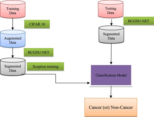
A dataset of gastric endoscopic images having IRB approval is taken from 69 patients in this work. The dataset contains around 480 images of which 230 images are applied for training and 240 are used for testing purposes. In the training set, there are 53 cancerous and 180 non-cancerous images whereas a test set has 30 cancerous and 190 non-cancerous images.

(A) Augmentation step

To overwhelm the overfitting of parameters in a neural network, the training data are not sufficient. So, augmenting the dataset inartificially using transformations that preserve the labels, a combination of image translation, flipping in the horizontal and vertical directions, shearing, rotation and cropping [25] randomly will reduce the overfitting problem. The AutoAugment tool of the google brain team helps in better data augmentation [28]. In this work, a variant of the CIFAR-10 policy is applied. To expand the dataset into 25 folds, 25 subpolicies are used. The techniques used in augment policy are given by Shear X/Y, Translate X/Y, Rotate, Auto Contrast, Invert, Equalize, Solarize, Posterize, Contrast, Colour, Brightness, Sharpness, Cut-out and Sample Pairing. Two parameters will give the probability value which will denote the likelihood of regulating the augmentation policy. Here, the invert is followed by contrast.

Invert operation has no magnitude data and the probability of applying is 0.1. Then, a Contrast of 0.2 is applied so we get a magnitude of 6 out of 10. There are 2.9 × 12 augmentation sub-policies [28], which are taken randomly and given to training data. To get the best policy, learning and classification are repeated to get improved performance.

Algorithm: CIFAR-10 policy

Step 1: The policy S is sampled by a recurrent neural network (RNN).

Step 2: Different types of augment policies are provided using a child network.

Step 3: The performance accuracy R is estimated and the controller RNN is updated to discover the finest augment policy.

Step 4: By the application of optimized data augmentation policies, high accuracy has been attained with public data.

(B) Segmentation

At first, CNN identifications and operations are provided. A detailed demonstration of the proposed BCGDU and its hyper-parameters are changed to advance the training task

CNN operations

• (1) CNN

In general, the human brain identifies the data to distinguish and classify the objects everywhere surrounding the human. Similarly, CNN (convolutional neural network) performs as a brain. It will not classify the objects without distinguishing the detailed data. CNN comprises convolution, activation, pooling, flattening and full connection. It is a feed-forward network with multiple layers. The connection among its neurons is stimulated by visual cortex association. Every neuron is ordered to answer to the interconnecting regions. The chief feature of CNNs is they involve grasping algorithms to grasp the image contents. They provide an enhanced representation of unstructured, information and provide a good ML classification which provides a correlation among labels. CNN will remove spatial correlation to develop new hidden data from the evident data. The CNN has convolutional and sub-sampling layers. Every layer has kernels to perform numerous alteration processes [29–42].

• (2) CNN components

A CNN architecture comprises CONV, pooling and FC layers. Every part has only one layer. FC layer has a global average pooling layer. This will reduce overfitting since parameters are not optimized and signify individual maps for every group. Various units for regulation given as BN and dropout are also implanted in the system to enhance CNN and remove overfitting. It is very essential to focus on organizing the components of CNN. This association improves performance.

CONV [43]: This layer has a group of kernelswhile help to divide the image into receptive fields. The kernel is provided to the input as numbers. The product operation of each and every kernel element with input tensor is done at all positions. The product is added to get the feature map. Zero paddings are applied for retaining in-plane dimensions, else each succeeding feature map will become smaller following this process.

Hyperparameters and down-sampling: The distance beteeen two kernel positions is called stride, which is greater than one to perform down-sampling. A pooling uses the size of kernels, number and padding, to perform down-sampling. At last, the output of the CONV layer is sent to activation functions such as Hyperbolic tangent, sigmoid,and ReLU which are not linear.

Pooling (PO) [44]: Pooling reduces the number of parameters, reduces the size of the feature map, preserves the complexity of the CNN, reduces overfitting and increases generalization. There are several methods, including MP, average pooling, global pooling, global average pooling, L2, overlapping and spatial pyramid pooling.

FC [45]: This layer flattens and transforms the output of the CONV and PO layers into a 1D array. The weight lies halfway between the input and the output. The final FC layer's output for the classification phase indicates the network's overall outcome, which represents the likely price of all classes. Output often has the same classes as input.

Gated recurrent unit (GRU)

Recurrent neural networks use gated recurrent units (GRUs) as their restrictions are imposed. The GRU has fewer parameters than an LSTM because it does not have an input gate, but it is similar to an LSTM with an output gate. The LSTM model's gated signals will be reduced by this GRU to just two. Update and reset gates are denoted by zt and rt, respectively. $\begin{array}{l}{z}_t=(w_x{X}_t+u_z{H_t}_{-1}+B_z)\\ r_t=(w_r{x}_t+u_r{H_t}_{-1}+B_r)\end{array}$This GRU has a three times increase in its parameters compared with recurrent neural networks. The total number of parameters is given by 3(N² + NM + N). This GRU outperforms the LSTM. The weights of gates are updated using back propagation through time, to minimize the cost function. There is a redundancy in driving these gate signals which are the internal state of the network.

The parameter will update the internal state of the system. There are some variants of GRU. In one variant, each gate is calculated by the previous hidden state and the bias. In the second variant, each gate is calculated only by the previous hidden state. In the third variant, the gate is calculated by bias. The total number of biases is reduced to 2(mn + n²).

BCGDU-Net

Inspired by U-Net [46], BConvL STM [47] and dense convolutions [48], we propose the BCGDU-Net, as shown in Figure 2. This network uses the combined effect of both the bi-directional ConvGRU and connected convolutions. The encoding path has four steps and every step has 3 × 3 filters followed by 2 × 2 max pooling functions and ReLU. At every step the feature map will be made twice. In this step, the representation of an image is extracted and the dimension of each layer is increased. The last layer will form higher dimensional image representations with high information. The U-Net has a set of convolutional layers to learn many features. The network did not learn the redundant features, it may learn in some other steps. To overcome this problem, dense convolution layers are used. By collective knowledge, i.e. reusing the feature maps such as concatenation of the feature maps from the preceding layer with the present layer and given to the next layer. The advantage of dense convolution is it can learn different features than redundant ones. This improves the system by reusing parameters. This prevents them from disappearing off the gradients. Here two convolutions are considered as one block. There is an arrangement of N blocks in the final layer. $x^i$ is the output of the layer whereas the input of the ith layer will be the concatenated value of feature maps. $x^i\in R^{F_1\ast W_1\ast H_1}$

Figure 2. BCDGU-Net.

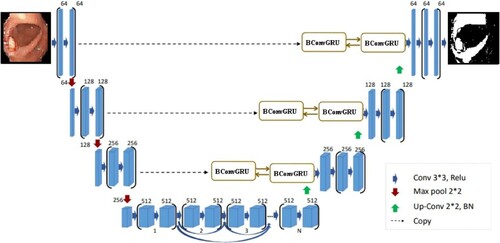
In the decoding step, every layer output is up-sampled. In U-Net the feature map of the encoding is taken to the decoding step. The concatenation of feature maps is done along with the result of up-sampling. In BCGDU-Net the following process occurs.

1. Let $x_e^i\in R^{F_l\ast W_l\ast H_l}$ be the set of feature maps taken from the encoding section, and $x_d^i\in R^{F_{l+1}\ast W_{l+1}\ast H_{l+1}}$ be the set of feature maps from the preceding convolutional layer, where $F_1,W_1\ast H_1$ is the number, and the size of each feature map at layer l, respectively. $\begin{array}{rl}& F_{l+1}=2^{\ast }{F}_l\\ & W_{l+1}={\frac{1}{2}}^{\ast }{W}_l\\ & H_{l+1}={\frac{1}{2}}^{\ast }{H}_l\end{array}$

The set of feature maps from the preceding layer is up-sampling followed by 2*2 convolution. In this, the size is made twice and the number of feature channels is made half. The features obtained are given by $x^u\in R^{F_{l+1}\ast W_{l+1}\ast H_{l+1}}$. The encoding path will increase the dimensions of the feature map so that it reaches actual size at the end of the final layer.

After the up-sampling process, the batch normalization function is done resulting in $x^{u1}\in R^{F_{l+1}\ast W_{l+1}\ast H_{l+1}}$. During the training phase in intermediate layers, a problem arises in distributing the activation function, as a result, the process becomes slow as it needs to adapt to every new activation function. The stability of the system will standardize the system by decreasing the mean from the standard deviation. This process will increase the speed of the system.

The output of the batch normalization stage is given to a BConvGRU layer. The standard GRU only considers the connections in input-to-state and state-to-state transitions but does not consider the spatial correlation. To avoid this difficult situation, ConvGRU [10] was projected. ConvGRU will exploit convolution into input-to-state and state-to-state transitions. It has i_t, o_t, f_t and c_t as the input gate, output gate, forget gate and memory cell, respectively. These gates are the controlling gates which help in accessing, updating and clearing memory cells. ConvGRU is given by $\begin{array}{rl}{i}_t& =\sigma \left({W_{\mathrm{xi}}}^{\ast }{x}_t+{W_{\mathrm{Hi}}}^{\ast }{h}_{t-1}+{W_{\mathrm{ci}}}^{\ast }{c}_{t-1}+{\text{B}}_{\text{i}}\right)\\ f_t& =\sigma \left({W_{\mathrm{xf}}}^{\ast }{x}_t+{W_{\mathrm{Hf}}}^{\ast }{h}_{t-1}+{W_{\mathrm{cf}}}^{\ast }{c}_{t-1}+{\text{B}}_{\text{f}}\right)\\ c_t& =f_{t^{\circ }}{c}_{t-1}+i_t\text{tanh}\left({W_{\mathrm{xc}}}^{\ast }{x}_t+{W_{\mathrm{Hc}}}^{\ast }{h}_{t-1}+{\text{B}}_{\text{c}}\right)\\ o_t& =\sigma ({W_{\mathrm{xo}}}^{\ast }{x}_t+{W_{\mathrm{Ho}}}^{\ast }{h}_{t-1}+W_{c{o}^{\circ }}{c}_t+{\text{B}}_0)\\ h_t& =o_t\in \text{tanh}\left(c_t\right),\end{array}$where *, , x_t, h_t, c_t, W_x∗, W_H∗ represent the convolution and Hadamard function, input tensor, hidden state tensor, memory cell tensor, 2-dimensional convolution kernel for input state, 2-dimensional convolution kernel for hidden state, respectively. B_i, B_f, B_c and B₀ are the bias terms.

BConvGRU helps to encode the input tensors. BConvGRU uses one ConvGRU to execute the data in a forward path others help to execute backward paths. But in the case of standard ConvGRU, data are processed in a forward path only. The entire data are considered so that the backward path will provide the best result. Both the forward and backward paths must be included in one ConvGRU. The output of the BConvGRU is planned as $y_t\text{ = tanh}\left(w_y^{\overrightarrow{h}}\ast \overrightarrow{h_t}+w_y^{\overleftarrow{h}}\overleftarrow{h_t}+b\right),$where $\overrightarrow{h_t}$ and $\overleftarrow{h_t}$ indicate the forward and backward states of the hidden state tensors, respectively, b is the bias term. The output will take into account the bidirectional special information. Moreover, tan h is the hyperbolic tangent form combination of forward and backward states. BCGDU-Net is used to train the network.

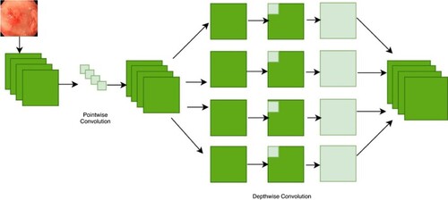
(C) Classification Xception network model

The Xception model's architecture is depicted in Figure 3. A CNN model called Xception, or “extreme inception”, uses the Inception module to weaken node connections and independently identify links between each channel by looking at local data. Inception module is displayed in Figure 4. The initialization module is responsible for separately turning on 1 × 1 and 3 × 3 convolution processes for every channel of the final feature map. The feature map for each channel will, therefore, be computed by the module. This module uses separable convolution to modify this procedure. To put on the 1 × 1 convolution is a point-wise convolution to the result, the depth-wise unique version will implement a combination process on all channels. Convolutions will produce separate feature maps for each channel when given the information from all channels and local data, and they will use a 1 × 1 convolution procedure to control the number of feature maps produced. The order of processes and the presence or lack thereof of intermediary activities, which are not linear by nature, are the key differences between the convolution layer. Figure 5 illustrates how explicit Xception is.

Figure 3. Xception architecture.

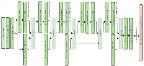
Figure 4. An extreme version of inception module.

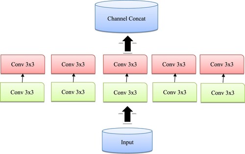
Figure 5. Concept of the Xception architecture.

The classification of stomach medical images using Xception yields the greatest results compared to other deep learning models such as Inception-V3, Resnet-101 and Inception-Resnet-V2. In addition, compared to ImageNet, SVHN and CIFAR-10, CIFAR-10's enhancement policy is the most successful one for the grouping task.

4. Result and discussion

The Kvasir dataset includes classes that represent anatomical and pathological findings and contains photos that have been reviewed by endoscopists. Z-line, pylorus, cecum and other anatomical landmarks are employed although oesophagitis, polyps, ulcerative colitis and other pathological findings are also used. Additionally, there are other sets of photos relating to the removal of lesions. The dataset includes photos with resolutions ranging from 720 × 578 to 1920 × 1074 pixels. The position of the endoscope in the intestine is depicted in green on fewer photographs using electromagnetic imaging methods that aid in image interpretation. Figure 6 lists the various forms of gastric lesions and Table 1 lists the number of Kvasir datastet-used lesions.

Figure 6. Types of images.

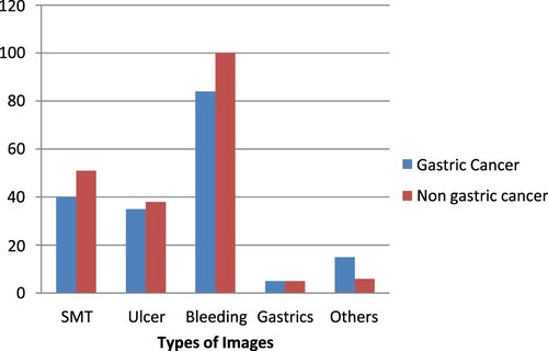
Table 1. The details of the Kvasir dataset.

Type of image		Number of images
Gastric cancer		65
Non-cancer	SMT	91
	Ulcer	73
	Bleeding	184
	Gastritis	10
	Others	21
Total		444

Pictures are enhanced during pre-processing. Every single image is enhanced into 25 images to comply with the CIFAR-10 policy. BCGDU-Net is used to segment each image once more. Data from the real world are taken into account while classifying and analysing the outcome. In the testing step, if more than one-third of the segmented area has cancer, the entire image is deemed to be malignant.

A threshold is set throughout the experiment since the cancer region may vary from patient to $\frac{\text{number}\text{of}\text{regions}\text{segmented}\text{as}\text{cancerous}}{\text{number}\text{of}\text{segmented}\text{regions}}\ge \frac{1}{3}$The data are augmented and segmented, and then the segmented data are recognized as whether cancerous or non-cancerous. As the size of lesion varies from patient to patient, there is a need for augmentation to identify the cancerous region from other gastric diseases. There are around 25 augmented sub-policies. The image is segmented into nine new images. Every image has one segmented region which has a higher pixel value. The comparison of the segmentation result is performed by augmentation, segmentation and by both of them. The region below the ROC curve is 0.92, 0.95 and 0.97 for augmentation, segmentation and proposed method, respectively. Figure 6 shows the results of ROC curves.

The deep learning toolbox package was used in Python to implement the network configuration. The programme took ∼1 h, ∼1 d, ∼3 h and ∼10 d to train 150 epochs for the original data, augmentation, segmentation, augmentation and segmentation, respectively. It took 47,000 iterations to train to have a mini- batch size of 65, and the learning rate was initially 0.002. The projected technique is faster than the other traditional methods. The proposed method is executed in 0.3 s. Google’s Auto Augment is found the best using reinforcement learning. A set of sub-policies are found good with the CIFAR-10 dataset and improve gastric cancer classification task. Numerous resources will form optimization in data augmentation.

We computed the sensitivity by cancer size and depth based on a prior study, as shown in Table 2.

Table 2. Cancer size and depth-based sensitivity.

Gastric cancer (mm)
Depth of cancer	≤10	10 = 15	11 = 20	≥25
Aug AUC	90	98.23	100	100
Seg AUC	90	94.12	95	96
Aug + Seg AUC	100	100	95	96

The respective specimen was used to calculate the sizes of the neoplasms (the major axis).

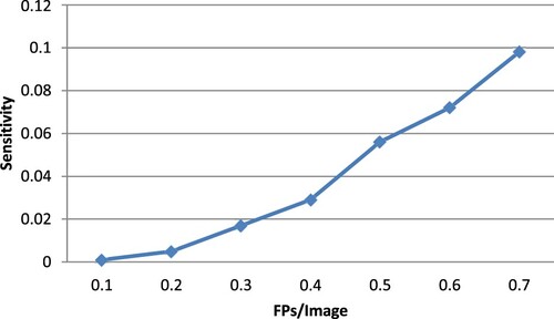
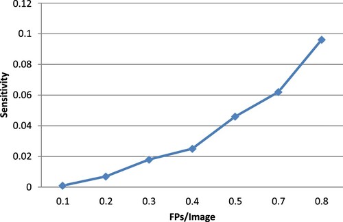
Figure 7 displays the detection outcomes for the suggested strategy, including successful detections, FPs and false negatives. The free-response receiver operator characteristic (FROC) curves, employing the numbers of FPs per image, the sensitivity based on the image and the sensitivity based on the lesion, are shown in Figure 8. Calculated from this curve, the sensitivities for image-based and lesion- based detections were 0.098 and 0.96, respectively.

Figure 7. The results of ROC curves.

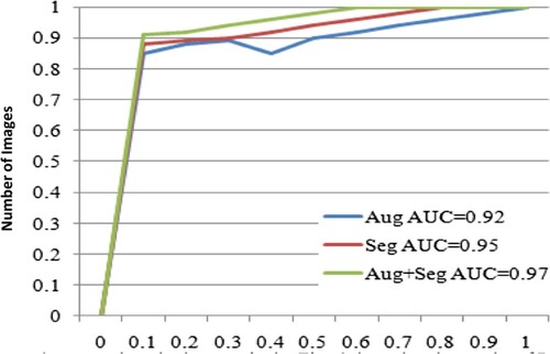
Figure 8. FROC curve image-based sensitivity.

The projected method's segmentation performance is correlated with fuzzy C means, global thresholding, BCGDNet and UNet. When compared to conventional procedures, the projected technique offers greater accuracy. The segmentation performance is compared in Table 2 with those of other methods, including fuzzy C means, global thresholding, BCD-Net and U Net.

To get rid of the FPs, the classification was applied to the 444 photos found during the initial detection. A sample cropped image that would be provided to CNN for FP reduction is shown in Figure 9.

Figure 9. FROC curve lesion-based sensitivity.

When an FP reduction was carried out using 3 distinct CNN architectures, the identification sensitivities and the number of FPs per picture and per lesion are shown in Table 2.

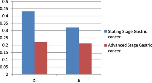
The best system to get rid of FPs was BCGDU-Net. Figure 10 displays examples of FPs that BCGDU-Net could remove and those that it could not. Table 3 displays the outcomes of the Di and Ji calculations for GC situations.

Figure 10. Proposed segmentation.

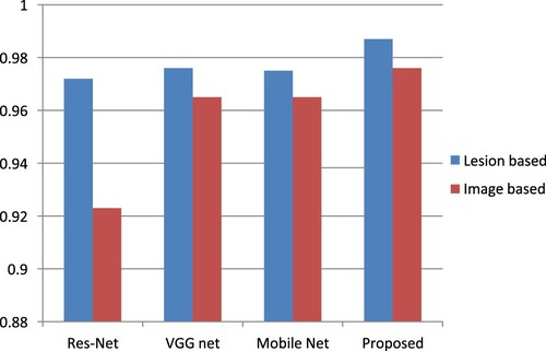
Table 3. A comparison of CNN architectures for the minimization of false positives.

	Sensitivity
Classifier	Lesion based	Image based	False positive
Res-Net	0.972	0.923	0.0321
VGG net	0.976	0.965	0.0452
Mobile Net	0.975	0.965	0.0412
Proposed	0.987	0.976	0.0511

In this paper, we suggested a BCGDU-Net for object detection and automatic GC case detection that integrates Res-Net, VGG-Net, Mobile-Net and an FP reduction algorithm (Figure 11).

Figure 11. False positive.

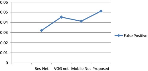
Using the BCGDU-Net output images, actual candidate regions were located using conventional background subtraction and labelling techniques and bounding boxes were made. To filter out FPs, CNN divided candidate areas into two categories: real GC cases and FPs. This method greatly outperformed the outcomes of the prior investigation, with a lesion-based sensitivity for the initial identification of 0.989 and several FPs per picture of 0.0511 (sensitivity, 0.987; the number of FPs per image, 0.976).

On the other hand, the study's use of Res-Net, VGG-Net and Mobile-Net allowed for the analysis of specific areas inside an image. Endoscopic pictures of the gastrointestinal mucosa were thoroughly analysed, and abnormal patterns were precisely identified.

Evaluation metrics

We assessed the results of the CNN models for picture segmentation and identification to verify the efficacy of the suggested approach. A confusion matrix was first built based on the CNN classification findings to assess the effectiveness of the CNN for image classification in the first stage. We determined the models’ precision, sensitivity, specificity and Jaccard Similarity Factor using the matrix.

Accuracy

The classifier's accuracy is the percentage of correct predictions it makes. It describes the overall performance of the classifier.

The following is how accuracy is defined: $\text{Accuracy}=\frac{(a_k+a_i)}{a_k+a_i+w_k+w_i)}$Sensitivity

Specificity $\text{specificity}=\frac{a_i}{a_i+w_k}$Precision $\text{precision}=\frac{a_k}{a_i+w_k}$F1-Score $F1\text{ - score}=\frac{2a_k}{\left(2a_k+w_k+w_i\right)}$Jaccard Similarity Coefficient $\mathrm{JAC}=\frac{a_k}{\left(a_k+w_k+w_i\right)}$The Hausdorff Distance is given by $k_{mod}(U,V)=\frac{1}{|U|}\sum _{\mathrm{usU}}^{min}\mathrm{vϵV}\parallel u-v\parallel$The above-mentioned indices were evaluated on an image-by-image (image-based) and case-by-case basis (case-based evaluation). The outcomes for the first scenario were computed after each image was allocated to the category with the greatest CNN output value. For the case-by-case analysis, the output values of the images acquired from a single case were averaged for each class, and the class with the highest average value was taken into account as the categorization outcome.

Using a feature map-based inference process represents higher modelling, a method for visualizing CNN output and determines which aspects of an image have an effect on the predictions. It can produce a stable activation map independent of the model and uses a variety of techniques, such as computing the CNN feature map's gradient, to identify the activation map. In this study, we calculated activation maps for healthy patients, upper gastrointestinal cancer patients and progressive gastric cancer patients to visualize the rationale for classification.

The grouping results show that the segmentation approaches provide improved results than the use of only the real image, indicating that the learning process over area labelling is active. It provides the potential for recognition techniques that will give lesion data using the probability of every patch (Table 4).

Table 4. Comparative segmentation performance with fuzzy C means, global thresholding, BCD-Net and U Net.

Method	Accuracy	Sensitivity	Specificity	Precision	FI-score
Fuzzy C means	0.9584	0.9585	0.9744	0.9998	0.977
Global thresholding	0.9612	0.9613	0.98310	0.9998	0.9801
BCD-Net	0.9674	0.9685	0.7985	0.9988	0.9832
U-Net	0.9771	0.9784	0.7533	0.9982	0.9882
Proposed method	0.9812	0.9856	0.9903	0.9999	0.9889

The accuracy, sensitivity, specificity, precision and F1 score of the proposed method are observed as 0.9812, 0.9856, 0.9903, 0.9999 and 0.9889, respectively. Table 5 shows the comparative classification performance with Res Net, VGG Net and Mobile Net. JAC, HD, accuracy, sensitivity and the specificity of the proposed Image Net are 0.8644, 8.9282, 0.98908 and 0.93756 respectively. Figures 12 and 13 show that the performance of the projected technique is higher than that of the existing technique.

Figure 12. Graphical plot for Table 2.

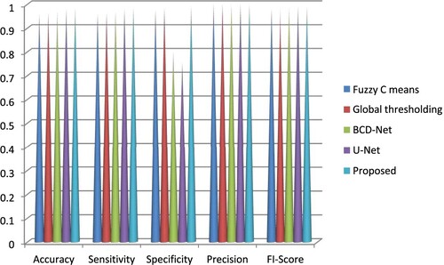
Figure 13. Graphical plot for Table 3.

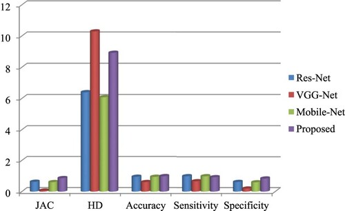
Table 5. Comparative chart of classification performance with Res-Net, VGG-Net and Mobile-Net.

Metrics	Res-Net	VGG-Net	Mobile-Net	Proposed
JAC	0.62598	0.06314	0.6055	0.86466
HD	6.4032	10.2955	6.0827	8.9282
Accuracy	0.94973	0.60839	0.9471	0.98908
Sensitivity	1	0.67238	1	0.93756
Specificity	0.62598	0.19638	0.6055	0.85153

The Area Under Curve (AUC) of classification shows how well it can distinguish between classes. The classifier can correctly distinguish between all positively and negatively labelled points if AUC = 1. The classifier views both positive and negative data as positive when the AUC is zero. The classifier has a decent chance of telling the difference between the pleasant and unpleasant possible values when AUC 1 is changed to 0.9, as shown in Figure 14.

Figure 14. Proposed AUC curve.

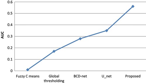
Figure 15. Stages of gastric cancer.

Be aware that healthy image segmentation frequently extracts false-positive zones. The evaluation's findings revealed that 25 healthy photos contained 415 false-positive regions, with an average number of false positives per image (FPI) of 0.0511.

Figure 15 displays the BCGDU-Net segmentation findings, while Table 6 lists the Dice and Jacquard parameters.

Table 6. Evaluation results of cancer segmentation.

	Di	Ji
Stating stage gastric cancer	0.432	0.321
Advanced stage gastric cancer	0.221	0.212

Images that are classified as healthy do not need to be segmented because the suggested method accomplishes the classification method in the initial stage. By eliminating the photos that were successfully categorized as healthy in the first stage, the false-positive regions from six images were removed, giving an FPI of 0.005 and the mistakes from the classification findings were studied.

The best performance was demonstrated by BCGDU-Net, which reduced FPs by almost 20% to 0.56 while retaining a lesion-based detection sensitivity of 0.096. Finally, we compared the performance of 4 different CNN designs. When measured using an image, the detection sensitivity decreased from 0.098 to 0.096 or around 4%.

Di and Ji examined the precision of extracting the invasion region of GC and found that for all GC images, the results were 0.55 and 0.42, respectively; however, when the test was limited to the photos that had been correctly identified, the results were 0.60 and 0.46, including both. When comparing all GC pictures, the proposed method outperformed the earlier research using BCGDU-Net; however the earlier research outperformed the proposed when comparing only the discovered regions. This suggests that while our technique may be able to detect minor lesions, it cannot precisely extract their forms.

To raise the extraction accuracy, it is necessary to improve the CNN model that was used for the automatic discovery and to perform post-processing, such as region growth, to the extracted images.

The suggested method yields a sensibility of 0.9856 in detecting GC while maintaining FPs at an acceptable level, which can assist in maintaining high examination accuracy in screening for GC by accounting for changes in physician skills.

5. Conclusion

In this paper, a CADx system is projected to differentiate and categorize cancerous cells from various gastric disorders. The system provided the Xception network, with individual convolutions. The projected technique used two methods: Google’s AutoAugment for data augmentation and BCGDU-Net for image segmentation. The augmentation and segmentation permitted the categorizing model to achieve enhanced results because this methodology prohibited overfitting. The segmented region is classified as cancerous or non-cancerous based on the features extracted in the training phase. This method is analysed with augmentation, segmentation and a combination of augmentation and segmentation. It is found that the area under the ROC curve for augmentation and segmentation is higher than those of the other two cases. Moreover, this technique provides a segmentation accuracy of 98% and a classification accuracy of 98.9%, which is higher than the existing techniques.

Disclosure statement

No potential conflict of interest was reported by the author(s).

References

- Krizhevsky A, Sutskever I, Geoffrey EH. ImageNet classification with deep convolutional neural networks. 2012. https://proceedings.neurips.cc/paper_files/paper/2012/file/c399862d3b9d6b76c8436e924a68c45b-Paper.pdf
- Ahmadi M, Vakili S, Langlois JMP, et al. Power reduction in CNN pooling layers with a preliminary partial computation strategy. Proceedings of the 16th IEEE International New Circuits and Systems Conference (NEWCAS); Jun 2018, p. 125–129.
- Balakrishnan G, Zhao A, Sabuncu MR, et al. VoxelMorph: a learning framework for deformable medical image registration. IEEE Trans Med Imag. Aug 2019;38(8):1788–1800. doi:10.1109/TMI.2019.2897538
- Bray F, Ferlay J, Soerjomataram I, et al. Global cancer statistics 2018: GLOBOCAN estimates of incidence and mortality worldwide for 36 cancers in 185 countries. CA Cancer J Clin. Nov 2018;68(6):394–424. doi:10.3322/caac.21492
- Asperti A, Mastronardo C. The effectiveness of data augmentation for detection of gastrointestinal diseases from endoscopical images. 2017, arXiv:1712.03689. [Online]. Available: http://arxiv.org/abs/1712.03689.
- Misumi A, Misumi K, Murakami A, et al. Endoscopic diagnosis of minute, small, and flat early gastric cancers. Endoscopy. Jul 1989;21:159–164.
- Honmyo U, Misumi A, Murakami A, et al. Mechanisms producing color change in flat early gastric cancers. Endoscopy. Jun 1997;29(5):366–371. doi:10.1055/s-2007-1004217
- Sahiner B, Pezeshk A, Hadjiiski LM, et al. Deep learning in medical imaging and radiation therapy. Med Phys. Jan 2019;46(1):e1–e36. doi:10.1002/mp.13264
- He K, Zhang X, Ren S, et al. Deep Residual Learning for Image Recognition. 2016.
- Khalid NEA, Samsudin N, Hashim R, et al. Abnormal gastric cell segmentation based on shape using morphological operations. In: Murgante B, editor. Computational science and its applications – ICCSA 2012. ICCSA 2012; 2012, pp. 728–738.
- Ishikawa T, Takahashi J, Takemura H, et al. Gastric lymph node cancer detection of multiple features classifier for pathology diagnosis support system. 2013 IEEE International Conference on Systems, Man, and Cybernetics; 2013, p. 2611–2616, doi:10.1109/SMC.2013.446
- He K, Zhang X, Ren S, et al. Deep residual learning for image recognition. 2016 IEEE Conference on Computer Vision and Pattern Recognition (CVPR); 2016, p. 770–778. doi:10.1109/CVPR.2016.90
- Oikawa K, Saito A, Kiyuna T, et al. Pathological diagnosis of gastric cancers with a novel computerized analysis system. J Pathol Inform. 2017;8:5. doi:10.4103/2153-3539.201114
- Choi IJ. Helicobacter pylori eradication therapy and gastric cancer prevention. Korean J Gastroenterol. Nov 2018;72:245–251. doi:10.4166/kjg.2018.72.5.245
- Cho B-J, Bang CS, Park SW, et al. Automated classification of gastric neoplasms in endoscopic images using a convolutional neural network. Endoscopy. Dec 2019;51(12):1121–1129. doi:10.1055/a-0981-6133
- Li L, Chen Y, Shen Z, et al. Convolutional neural network for the diagnosis of early gastric cancer based on magnifying narrow band imaging. Gastric Cancer. Jan 2020;23(1):126–132. doi:10.1007/s10120-019-00992-2
- Cubuk ED, Zoph B, Mane D, et al. Autoaugment: learning augmentation strategies from data. Proceedings of IEEE/CVFConference Computer Vision Pattern Recognition (CVPR); Jun 2019, p. 113–123.
- Chollet F. Xception: deep learning with depthwise separable convolutions. Proceedings of the IEEE Conference on Computer Vision and Pattern Recognition (CVPR); Jul 2017, p. 1251–1258.
- Ergashev D, Cho YI. Skin lesion classification towards melanoma diagnosis using convolutional neural network and image enhancement methods. J Korean Inst Intell Syst. Jun 2019;29(3):204–209.
- Fitzmaurice C, Akinyemiju TF, Al Lami FH, et al. Global, regional, and national cancer incidence, mortality, years of life lost, years lived with disability, and disability-adjusted life-years for 29 cancer groups, 1990 to 2016: a systematic analysis for the global burden of disease study global burden of disease cancer collaboration. JAMA Oncol 2018;4:1553–1568. doi:10.1001/jamaoncol.2018.2706
- Frid-Adar M, Diamant I, Klang E, et al. GAN-based synthetic medical image augmentation for increased CNN performance in liver lesion classification. Neurocomputing. Dec 2018;321:321–331. doi:10.1016/j.neucom.2018.09.013
- Kanesaka T, Lee T-C, Uedo N, et al. Computer-aided diagnosis for identifying and delineating early gastric cancers in magnifying narrow-band imaging. Gastrointest Endosc. May 2018;87(5):1339–1344. doi:10.1016/j.gie.2017.11.029
- Ko K-P. Epidemiology of gastric cancer in Korea. J Korean Med Assoc. Aug 2019;62:398–406. doi:10.5124/jkma.2019.62.8.398
- Khryashchev VV, Stepanova OA, Lebedev AA, et al. Deep learning for gastric pathology detection in endo-scopic images. Proceedings of the 3rd International Conference on Graphical Signal Processing; Jun. 2019, p. 90–94.
- Krizhevsky A, Sutskever I, Hinton GE. Imagenet classification with deep convolutional neural networks. Proceedings of the Advanced Neural Information Processing System (NIPS); 2012, p. 1097–1105.
- Kim D-H, Cho H, Cho H-C. Gastric lesion classification using deep learning based on fast and robust fuzzy C-means and simple linear iterative clustering superpixel algorithms. J Electr Eng Technol. Nov 2019;14(6):2549–2556. doi:10.1007/s42835-019-00259-x
- Liu W, Anguelov D, Erhan D, et al. SSD: single shot multibox detector. Proceedings of the European Conference Computer Vision; 2016, p. 21–37.
- Wang H, Ding S, Wu D, et al. Smart connected electronic gastroscope system for gastric cancer screening using multi-column convolutional neural networks. Int J Prod Res. 2019;57(21):6795–6806. doi:10.1080/00207543.2018.1464232
- Khan A, Sohail A, Zahoora U, et al. A survey of the recent architectures of deep convolutional neural networks. Artif Intell Rev. Dec 2020;53(8):5455–5516. doi:10.1007/s10462-020-09825-6
- Chowdhary CL, Mittal M, Pattanaik PA, et al. An efficient segmentation and classification system in medical images using intuitionist possibilistic fuzzy C-mean clustering and fuzzy SVM algorithm. Sensors. Jul 2020;20(14):3903. doi:10.3390/s20143903
- Kim D-H, Cho H-C. Deep learning based computer-aided diagnosis system for gastric lesion using endoscope. Trans Korean Inst Electr Eng. 2018;67(7):928–933.
- Lee S, Chin Cho H, Chong Cho H. A novel approach for increased convolutional neural network performance in gastric-cancer classification using endoscopic images. IEEE Access. 2021;9:51847–51854. doi:10.1109/ACCESS.2021.3069747
- Hirasawa T, Aoyama K, Tanimoto T, et al. Application of artificial intelligence using a convolutional neural network for detecting gastric cancer in endoscopic images. Gastric Cancer. 2018;21:653–660. doi:10.1007/s10120-018-0793-2
- Jin Z, Gan T, Wang P, et al. Deep learning for gastroscopic images: computer-aided techniques for clinicians. Biomed Eng Online. 2022;21:12. doi:10.1186/s12938-022-00979-8
- Sakai Y, Takemoto S, Hori K, et al. Automatic detection of early gastric cancer in endoscopic images using a transferring convolutional neural network. Proceedings of the 2018 40th Annual International Conference of the IEEE Engineering in Medicine and Biology Society (EMBC); 18–21 Jul 2018; Honolulu, HI, USA; p. 4138–4141.
- Shibata T, Teramoto A, Yamada H, et al. Automated detection and segmentation of early gastric cancer from endoscopic images using mask R-CNN. Appl Sci. 2020;10:3842. doi:10.3390/app10113842
- Teramoto A, Shibata T, Yamada H, et al. Automated detection of gastric cancer by retrospective endoscopic image dataset using U-Net R-CNN. Appl Sci. 2021;11:11275. doi:10.3390/app112311275
- Ungureanu B, Sacerdotianu V, Turcu-Stiolica A, et al. Endoscopic ultrasound vs. computed tomography for gastric cancer staging: a network meta-analysis. Diagnostics. 2021;11:134. doi:10.3390/diagnostics11010134
- Hamada K, Kawahara Y, Tanimoto T, et al. Application of convolutional neural networks for evaluating the depth of invasion of early gastric cancer based on endoscopic images. Gastroenterol Hepatol. 2022;37:352–357. doi:10.1111/jgh.15725
- Hirai K, Kuwahara T, Furukawa K, et al. Artificial intelligence-based diagnosis of upper gastrointestinal subepithelial lesions on endoscopic ultrasonography images. Gastric Cancer. 2022;25:382–391. doi:10.1007/s10120-021-01261-x
- Zhu Y, Wang Q-C, Xu M-D, et al. Application of convolutional neural network in the diagnosis of the invasion depth of gastric cancer based on conventional endoscopy. Gastrointest Endosc. 2019;89(4):806–815. doi:10.1016/j.gie.2018.11.011
- Zhao A, Balakrishnan G, Durand F, et al. Data augmentation using learned transformations for one-shot medical image segmentation. Procedings of the IEEE/CVF Conference Computer Vision Pattern Recognition (CVPR); Jun 2019, p. 8543–8553.
- Srinivas S, Sarvadevabhatla RK, Mopuri KR, et al. An introduction to deep convolutional neural nets for computer vision. In: SK Zhou, H Greenspan, D Shen, editor. Deep learning for medical image analysis. New York (NY): Academic; 2017, ch. 2, pp. 25–52.
- Yamashita R, Nishio M, Do RKG, et al. Convolutional neural networks: an overview and application in radiology. Insights IntoImag. Aug 2018;9(4):611–629.
- Huang G, Liu Z, Van Der Maaten L, et al. Densely connected convolutional networks. Proceedings of the IEEE Conference on Computer Vision and Pattern Recognition; 2017, p. 4700–4708.
- Song H, Wang W, Zhao S, et al. Pyramid dilated deeper convlstm for video salient object detection. Proceedings of the European Conference on Computer Vision (ECCV); 2018, p. 715–731.
- Yoon HJ, Kim S, Kim J-H, et al. A lesion-based convolutional neural network improves endoscopic detection and depth prediction of early gastric cancer. J Clin Med. 2019;8:1310. doi:10.3390/jcm8091310
- Ronneberger O, Fischer P, Brox T. U-net: convolutional networks for biomedical image segmentation. International Conference on Medical Image Computing and Computer-Assisted Intervention; 2015. Springer, p. 234–241.