Position sensorless extended and unscented Kalman filters with permanent magnet flux linkage and load torque estimation for surface-mounted PMSM

Abstract

In this paper, novel position sensorless state estimators with improved robustness to permanent magnet (PM) flux linkage variations in permanent magnet synchronous machines (PMSMs) are presented. Unlike state estimators using conventional infinite inertia or electromechanical models, the estimators presented here can also estimate the PM flux linkage, so they are not sensitive to its uncertainty. For each models used for state estimation, a detailed observability study is presented. Due to the nonlinear models, extended and unscented Kalman filter algorithms are used for the implementation. To compare the sensitivity of conventional and proposed state estimators to uncertainty in electrical parameters, numerical simulations are carried out. In addition, the computational burden of the estimators is compared by real-time execution.

Keywords:

• Permanent magnet synchronous machine
• position sensorless state estimation
• permanent magnet flux linkage estimation
• load torque estimation
• nonlinear observability
• extended and unscented Kalman filters

1. Introduction

Estimators and observers are widely used in controlled permanent magnet synchronous machine (PMSM) drives to determine the required quantities without direct measurement. One such application is the online parameter estimation, since the control performance depends on the accurate knowledge of the machine parameters. However, these parameters can change during the operation. For example, permanent magnet (PM) flux linkage decreases and the stator winding resistance increases at high temperatures, as well as the inductances vary due to the magnetic saturation in PMSMs. To compensate the effect of parameter mismatches, online parameter estimations are often used. The most important methods are reviewed in [1]. Besides parameter uncertainties, load disturbances have also significant impact on performance. To improve dynamics and reduce the impact of load variations, extended state observer-based disturbance rejection techniques are used in [2, 3]. These works compensate the output of the speed controller by the estimated value of load torque. As a result, the effect of load disturbance is much less on speed control performance.

Model-based estimators are also often used to improve the robustness of the drive system against sensor faults. In [4], a sliding mode observer (SMO) is used to estimate the position and speed of the rotor from the measured terminal voltages and currents. By comparing the estimated values with their measured counterparts, the fault of the position sensor can be detected. In case of a faulty sensor, the fault tolerant PMSM drive uses the estimated position and speed instead of the sensor output. Although the velocity and position sensors can be fully replaced by estimators. These position sensorless methods can be useful, e.g. if the size of the sensor makes it difficult to install the drive or if a low-maintenance and high-reliability system is recommended due to the harsh operating environment. One such tidal power application is shown in [5]. Further advantages of position sensorless drives are the increased noise immunity and the reduced cost, as described in [6]. The model-based position sensorless estimators can be implemented in open-loop or in closed-loop structures. The open-loop estimators are simpler and require less computational efforts, but these methods have worse dynamic performance and are highly sensitive to measurement errors and parameter uncertainties. In contrary, the Luenberger-type observers in [7, 8], the SMOs in [9, 10], as well as the nonlinear Kalman filters in [11, 12] have closed-loop structure, which reduces the effect of model inaccuracies. In addition, Kalman filter-type estimators use noise models to take into account the stochastic behaviour of the process and the measurement. However, this feature increases the computational complexity and makes tuning more difficult. It is important to point out that the accuracy of the model-based position sensorless estimators deteriorates at low speeds, where performance can be improved by signal injection-based methods as in [13]. However, signal injection causes unwanted torque ripples, increased losses and acoustic noises as mentioned in [14]. Signal injection is therefore recommended only at start-up and at low speed, but at medium and high speeds it is worth switching to a model-based estimation method.

In terms of modelling mechanical behaviour, there are two main groups of models used to design position sensorless state estimators. The first is the so-called infinite inertia model, which uses only the electrical equations and considers the rotor velocity as a slowly varying quantity. This approximation can often be applied, because the electrical time constants in PMSM drives are usually much smaller than the mechanical ones. An important advantage of the infinite inertia hypothesis is that the modelling does not require the identification of mechanical parameters, as these are not used. Applying this modelling approach to the surface-mounted PMSM, stochastic state estimators are developed using extended Kalman filter (EKF) in [11] and unscented Kalman filter (UKF) in [12]. A detailed observability analysis of the infinite inertia model can be found in [15]. The second type of models used for position sensorless state estimation includes the equation of motion. This model is usually called electromechanical or full model. Since the load torque is included in the equation of motion, it can be defined as an additional state variable. As a result, the load torque can be estimated and used to improve the speed control performance as shown in [16]. An observability study of the electromechanical model is presented in [17], with particular attention to observability conditions at zero speed.

The main drawback of position sensorless model-based estimators is their sensitivity to parameter uncertainties. In other words, the performance of the estimator is reduced if the machine parameters implemented in the estimator differ from the actual values. To reduce sensitivity, position and speed estimation can be combined with parameter estimation. In [18], an extended electromotive force model-based estimator is used, which is quite sensitive to the stator resistance variation, particularly at low speeds. To improve performance, the estimator is combined with an online resistance identifier using the recursive least squares method. In [19], an adaptive SMO is proposed in which the resistance value can be adjusted adaptively to achieve lower sensitivity. The combination of position and parameter estimators results in a complex structure. In contrast, Kalman filters can be easily extended for parameter estimation by defining the parameter to be estimated as an additional state variable. In [20], an augmented electromechanical model-based nonlinear Kalman filter is proposed, which is extended for stator resistance estimation. Using resistance estimation for adaptive control and estimated load torque for disturbance rejection, improved speed control performance can be achieved. But the negative effects are not only due to the inaccuracy of the resistance. As shown in [21], the effect of a decrease in magnetism is more dominant than the effect of resistance variation in model predictive control. In [22], the PM flux linkage is identified online by an EKF using the velocity from the model reference adaptive estimator. In contrast, a joint EKF is used to estimate the PM flux linkage, load torque, velocity and position in [23]. The EKF-based model predictive speed control of PMSM is thus robust to PM flux linkage and load torque variations. In summary, the performance of position and velocity estimators can be improved by parameter estimation. In such cases, it is important that observable models are used for estimation, as only then can the state vector be fully reconstructed from the measurements. However, a shortcoming of [18–20, 22, 23] is that the observability of the models used for estimation is not analyzed.

In this paper, position sensorless state estimators for surface-mounted PMSM are presented and compared. Different estimators use different state-space models. In this way, it is possible to estimate not only the position and velocity but also the load torque and the PM flux linkage. The four different models used are the well-known infinite inertia and electromechanical models, as well as augmented versions of these models. In augmented models, the PM flux linkage is an additional state variable. Using these augmented models reduces the sensitivity of the estimators to PM flux linkage variations. The main contributions of this study are as follows:

• Novel position sensorless state estimators are presented, which are robust to PM flux linkage and load variations.

• A detailed observability study is presented for different state-space representations used in different estimators.

• Numerical simulations are performed to compare the parameter sensitivities.

• Extended and unscented Kalman filters are compared and it is shown that their performance is nearly identical for surface-mounted PMSM. The estimation performance depends mainly on the model used.

The author discloses that this study extends the results of former conference paper [24]. For completeness, a fourth model is presented for estimation. The observability study is thus extended. Furthermore, the estimation performances using EKF and UKF are also compared, and the sensitivities to all electrical parameters are investigated. In addition, the computational burden of the estimators is compared by real-time execution.

2. Observability analysis of PMSM models used to design estimators

In this section, four different state-space models of surface-mounted PMSMs are presented. These models are used for position sensorless state estimation, so it is important to ensure that the models are observable, because only then can the state vector be fully reconstructed from the measurement. Therefore, detailed observability studies are also presented for these models.

To describe the electromagnetic behaviour of a PMSM, different coordinate systems can be used. Obvious choices could be the reference frame of the stator or the rotor. The later is often used for vector control, because the stator current vector can be divided into flux and torque producing components. However, stationary reference frame is more popular for estimator design, because the derivative of the stator currents are linearly related to both currents and excitation voltages, as mentioned in [11]. It is also important that the inductance is independent of the rotor direction in case of the surface-mounted PMSM, unlike salient-pole machines. Therefore, the use of the rotor reference frame is not justified. In addition, observability can be easily ensured if all the electrical variables are specified in stationary reference frame.

The voltage equations of surface-mounted PMSM in stationary two-axis reference frame are (1) $u_{\alpha }=R{i}_{\alpha }+L\frac{\mathrm{d}{i}_{\alpha }}{\mathrm{d}t}-\lambda {\omega }_e\sin \left({\phi }_e\right)$(1) and (2) $u_{\text{β}}=R{i}_{\text{β}}+L\frac{\mathrm{d}{i}_{\text{β}}}{\mathrm{d}t}+\lambda {\omega }_e\cos \left({\phi }_e\right),$(2) where $u_{\alpha }$, $u_{\text{β}}$ and $i_{\alpha }$, $i_{\text{β}}$ are the stator voltage and current components, as well as, ${\phi }_e$ and ${\omega }_e$ denote the electrical position and velocity of the rotor, respectively. In (1(1) $u_{\alpha }=R{i}_{\alpha }+L\frac{\mathrm{d}{i}_{\alpha }}{\mathrm{d}t}-\lambda {\omega }_e\sin \left({\phi }_e\right)$(1) ) and (2(2) $u_{\text{β}}=R{i}_{\text{β}}+L\frac{\mathrm{d}{i}_{\text{β}}}{\mathrm{d}t}+\lambda {\omega }_e\cos \left({\phi }_e\right),$(2) ), R is the stator resistance, L is stator inductance and λ is the PM flux linkage. By using the stator current components given in the stationary reference frame, the electromagnetic torque of a three-phase surface-mounted PMSM can be determined as (3) $T_{\mathrm{em}}=\frac{3}{2}\mathrm{p\lambda }(i_{\text{β}}\cos ({\phi }_e)-i_{\alpha }\sin ({\phi }_e\left)\right),$(3) where p is the number of pole pairs.

To describe the dynamics of the rotor, the equation of motion is used as (4) $\frac{\mathrm{d}{\omega }_e}{\mathrm{d}t}=\frac{p{T}_{\mathrm{em}}-D{\omega }_e-p{T}_L}{J},$(4) where D, $T_L$ and J are the viscous friction coefficient, the load torque, as well as the total inertia of the rotor and the load, respectively.

In (1(1) $u_{\alpha }=R{i}_{\alpha }+L\frac{\mathrm{d}{i}_{\alpha }}{\mathrm{d}t}-\lambda {\omega }_e\sin \left({\phi }_e\right)$(1) )–(3(3) $T_{\mathrm{em}}=\frac{3}{2}\mathrm{p\lambda }(i_{\text{β}}\cos ({\phi }_e)-i_{\alpha }\sin ({\phi }_e\left)\right),$(3) ), trigonometric functions and multiplications of variables result in nonlinear terms, which are also included in the state-space models used to design estimators. Therefore, the locally weak observability is used to analyze the nonlinear state-space representations, as in [15, 24]. A brief description of this approach is given below.

The state-space model of a nonlinear system in continuous time can be written as (5) $\begin{array}{rl}\frac{\mathrm{d}\mathit{x}}{\mathrm{d}t}& =\mathit{f}(\mathit{x},\mathit{u}),\end{array}$(5) (6) $\begin{array}{rl}\mathit{y}& =\mathit{h}(\mathit{x},\mathit{u}),\end{array}$(6) where $\mathit{f}(\mathit{x},\mathit{u})$ and $\mathit{h}(\mathit{x},\mathit{u})$ are given nonlinear functions of $\mathit{x}$ state and $\mathit{u}$ input vectors, as well as $\mathit{y}$ denotes the output vector. For the model (5(5) $\begin{array}{rl}\frac{\mathrm{d}\mathit{x}}{\mathrm{d}t}& =\mathit{f}(\mathit{x},\mathit{u}),\end{array}$(5) ) and (6(6) $\begin{array}{rl}\mathit{y}& =\mathit{h}(\mathit{x},\mathit{u}),\end{array}$(6) ), the observability matrix is (7) $\mathcal{O}={\left[\begin{array}{cccc}{\displaystyle \frac{\mathrm{\partial }{\mathcal{L}}_{\mathit{f}}^0\mathit{h}}{\mathrm{\partial }\mathit{x}}}& {\displaystyle \frac{\mathrm{\partial }{\mathcal{L}}_{\mathit{f}}\mathit{h}}{\mathrm{\partial }\mathit{x}}}& \cdots & {\displaystyle \frac{\mathrm{\partial }{\mathcal{L}}_{\mathit{f}}^{n-1}\mathit{h}}{\mathrm{\partial }\mathit{x}}}\end{array}\right]}^{\mathrm{T}},$(7) where ${\mathcal{L}}_{\mathit{f}}^k\mathit{h}$ denotes kth order Lie derivative of function $\mathit{h}$ with respect to the vector field $\mathit{f}$, and n is the dimension of the state-space. The model (5(5) $\begin{array}{rl}\frac{\mathrm{d}\mathit{x}}{\mathrm{d}t}& =\mathit{f}(\mathit{x},\mathit{u}),\end{array}$(5) ) and (6(6) $\begin{array}{rl}\mathit{y}& =\mathit{h}(\mathit{x},\mathit{u}),\end{array}$(6) ) is locally weakly observable at $x_0$, if the rank condition (8) $\mathrm{rank}{\left\{\mathcal{O}\right\}|}_{x_0}=n$(8) is fulfilled.

2.1. Infinite inertia model

The simplest state-space model used to design position sensorless state estimator is based only on voltage equations (1(1) $u_{\alpha }=R{i}_{\alpha }+L\frac{\mathrm{d}{i}_{\alpha }}{\mathrm{d}t}-\lambda {\omega }_e\sin \left({\phi }_e\right)$(1) ) and (2(2) $u_{\text{β}}=R{i}_{\text{β}}+L\frac{\mathrm{d}{i}_{\text{β}}}{\mathrm{d}t}+\lambda {\omega }_e\cos \left({\phi }_e\right),$(2) ) and assumes the infinite inertia hypothesis. Accordingly, the electrical variables change much faster than the angular velocity. Therefore, $\frac{\mathrm{d}{\omega }_e}{\mathrm{d}t}=0$ can be written in the state equation. Since ${\omega }_e$ is the first order derivative of ${\phi }_e$, and by choosing stator currents, angular velocity and position as state variables, the state equation of infinite inertia model is (9) $\frac{\mathrm{d}}{\mathrm{d}t}\left[\begin{array}{c}{i}_{\alpha }\\ i_{\text{β}}\\ {\omega }_e\\ {\phi }_e\end{array}\right]=\left[\begin{array}{c}{\displaystyle \frac{1}{L}{u}_{\alpha }-{\displaystyle \frac{R}{L}{i}_{\alpha }+{\displaystyle \frac{\lambda }{L}{\omega }_e\sin \left({\phi }_e\right)}}}\\ {\displaystyle \frac{1}{L}{u}_{\text{β}}-{\displaystyle \frac{R}{L}{i}_{\text{β}}-{\displaystyle \frac{\lambda }{L}{\omega }_e\cos \left({\phi }_e\right)}}}\\ 0\\ {\omega }_e\end{array}\right].$(9) The inputs of this model are $u_{\alpha }$, $u_{\text{β}}$ voltages, and the outputs are $i_{\alpha }$, $i_{\text{β}}$ stator currents for position sensorless application.

The observability matrix of the infinite inertia model can be written as (10) $\mathcal{O}=\left[\begin{array}{cccc}{\displaystyle \frac{\mathrm{\partial }{\mathcal{L}}_{\mathit{f}}^0\mathit{h}}{\mathrm{\partial }{i}_{\alpha }}}& {\displaystyle \frac{\mathrm{\partial }{\mathcal{L}}_{\mathit{f}}^0\mathit{h}}{\mathrm{\partial }{i}_{\text{β}}}}& {\displaystyle \frac{\mathrm{\partial }{\mathcal{L}}_{\mathit{f}}^0\mathit{h}}{\mathrm{\partial }{\omega }_e}}& {\displaystyle \frac{\mathrm{\partial }{\mathcal{L}}_{\mathit{f}}^0\mathit{h}}{\mathrm{\partial }{\phi }_e}}\\ {\displaystyle \frac{\mathrm{\partial }{\mathcal{L}}_{\mathit{f}}\mathit{h}}{\mathrm{\partial }{i}_{\alpha }}}& {\displaystyle \frac{\mathrm{\partial }{\mathcal{L}}_{\mathit{f}}\mathit{h}}{\mathrm{\partial }{i}_{\text{β}}}}& {\displaystyle \frac{\mathrm{\partial }{\mathcal{L}}_{\mathit{f}}\mathit{h}}{\mathrm{\partial }{\omega }_e}}& {\displaystyle \frac{\mathrm{\partial }{\mathcal{L}}_{\mathit{f}}\mathit{h}}{\mathrm{\partial }{\phi }_e}}\\ {\displaystyle \frac{\mathrm{\partial }{\mathcal{L}}_{\mathit{f}}^2\mathit{h}}{\mathrm{\partial }{i}_{\alpha }}}& {\displaystyle \frac{\mathrm{\partial }{\mathcal{L}}_{\mathit{f}}^2\mathit{h}}{\mathrm{\partial }{i}_{\text{β}}}}& {\displaystyle \frac{\mathrm{\partial }{\mathcal{L}}_{\mathit{f}}^2\mathit{h}}{\mathrm{\partial }{\omega }_e}}& {\displaystyle \frac{\mathrm{\partial }{\mathcal{L}}_{\mathit{f}}^2\mathit{h}}{\mathrm{\partial }{\phi }_e}}\\ {\displaystyle \frac{\mathrm{\partial }{\mathcal{L}}_{\mathit{f}}^3\mathit{h}}{\mathrm{\partial }{i}_{\alpha }}}& {\displaystyle \frac{\mathrm{\partial }{\mathcal{L}}_{\mathit{f}}^3\mathit{h}}{\mathrm{\partial }{i}_{\text{β}}}}& {\displaystyle \frac{\mathrm{\partial }{\mathcal{L}}_{\mathit{f}}^3\mathit{h}}{\mathrm{\partial }{\omega }_e}}& {\displaystyle \frac{\mathrm{\partial }{\mathcal{L}}_{\mathit{f}}^3\mathit{h}}{\mathrm{\partial }{\phi }_e}}\end{array}\right].$(10) Since the function $\mathit{h}$ expresses two output variables, each element of the matrix $\mathcal{O}$ is actually a two element vector. Therefore, the total number of rows in matrix $\mathcal{O}$ is 8. If this matrix $\mathcal{O}$ has full rank, then the infinite inertia model is locally weakly observable. To satisfy the rank condition $\mathrm{rank}\left\{\mathcal{O}\right\}=4$, there must be at least one regular matrix that can be constructed from 4 different rows of $\mathcal{O}$. In this way, 70 different $4\times 4$ matrices can be created from the 8 rows. Among these matrices, an important result is obtained from the analysis of matrix ${\mathcal{O}}_{1-4}$, which consists of the first 4 rows of matrix $\mathcal{O}$. The determinant of ${\mathcal{O}}_{1-4}$ is (11) $\det \left\{{\mathcal{O}}_{1-4}\right\}=\frac{{\lambda }^2}{L^2}{\omega }_e.$(11) If $\det \left\{{\mathcal{O}}_{1-4}\right\}\ne 0$, then ${\mathcal{O}}_{1-4}$ is regular and matrix $\mathcal{O}$ has full rank, so the model (9(9) $\frac{\mathrm{d}}{\mathrm{d}t}\left[\begin{array}{c}{i}_{\alpha }\\ i_{\text{β}}\\ {\omega }_e\\ {\phi }_e\end{array}\right]=\left[\begin{array}{c}{\displaystyle \frac{1}{L}{u}_{\alpha }-{\displaystyle \frac{R}{L}{i}_{\alpha }+{\displaystyle \frac{\lambda }{L}{\omega }_e\sin \left({\phi }_e\right)}}}\\ {\displaystyle \frac{1}{L}{u}_{\text{β}}-{\displaystyle \frac{R}{L}{i}_{\text{β}}-{\displaystyle \frac{\lambda }{L}{\omega }_e\cos \left({\phi }_e\right)}}}\\ 0\\ {\omega }_e\end{array}\right].$(9) ) is locally weakly observable. Since λ and L are positive constants in the infinite inertia model, condition ${\omega }_e\ne 0$ ensures the locally weak observability. This well-known condition is the same as in [15]. It is also important to note that the rank of $\mathcal{O}$ decreases in stationary position: (12) ${\mathrm{rank}\left\{\mathcal{O}\right\}|}_{{\omega }_e=0}=3.$(12) Therefore, ${\omega }_e\ne 0$ is a necessary and sufficient condition for locally weak observability.

2.2. Infinite inertia model augmented by PM flux linkage

In state estimators, such as Kalman filters, the state variables of the applied model are estimated. So, these types of estimators can be easily extended to joint parameter estimation by choosing the parameter to be estimated as a state variable. In this way, the conventional infinite inertia model can be augmented for PM flux linkage estimation as (13) $\frac{\mathrm{d}}{\mathrm{d}t}\left[\begin{array}{c}{i}_{\alpha }\\ i_{\text{β}}\\ {\omega }_e\\ {\phi }_e\\ \lambda \end{array}\right]=\left[\begin{array}{c}{\displaystyle \frac{1}{L}{u}_{\alpha }-{\displaystyle \frac{R}{L}{i}_{\alpha }+{\displaystyle \frac{\lambda }{L}{\omega }_e\sin \left({\phi }_e\right)}}}\\ {\displaystyle \frac{1}{L}{u}_{\text{β}}-{\displaystyle \frac{R}{L}{i}_{\text{β}}-{\displaystyle \frac{\lambda }{L}{\omega }_e\cos \left({\phi }_e\right)}}}\\ 0\\ {\omega }_e\\ 0\end{array}\right],$(13) in which a slowly varying PM flux linkage is assumed.

Since the state vector is augmented by λ, the observability matrix is (14) $\begin{array}{r}\mathcal{O}=\left[\begin{array}{ccccc}{\displaystyle \frac{\mathrm{\partial }{\mathcal{L}}_{\mathit{f}}^0\mathit{h}}{\mathrm{\partial }{i}_{\alpha }}}& {\displaystyle \frac{\mathrm{\partial }{\mathcal{L}}_{\mathit{f}}^0\mathit{h}}{\mathrm{\partial }{i}_{\text{β}}}}& {\displaystyle \frac{\mathrm{\partial }{\mathcal{L}}_{\mathit{f}}^0\mathit{h}}{\mathrm{\partial }{\omega }_e}}& {\displaystyle \frac{\mathrm{\partial }{\mathcal{L}}_{\mathit{f}}^0\mathit{h}}{\mathrm{\partial }{\phi }_e}}& {\displaystyle \frac{\mathrm{\partial }{\mathcal{L}}_{\mathit{f}}^0\mathit{h}}{\mathrm{\partial }\lambda }}\\ {\displaystyle \frac{\mathrm{\partial }{\mathcal{L}}_{\mathit{f}}\mathit{h}}{\mathrm{\partial }{i}_{\alpha }}}& {\displaystyle \frac{\mathrm{\partial }{\mathcal{L}}_{\mathit{f}}\mathit{h}}{\mathrm{\partial }{i}_{\text{β}}}}& {\displaystyle \frac{\mathrm{\partial }{\mathcal{L}}_{\mathit{f}}\mathit{h}}{\mathrm{\partial }{\omega }_e}}& {\displaystyle \frac{\mathrm{\partial }{\mathcal{L}}_{\mathit{f}}\mathit{h}}{\mathrm{\partial }{\phi }_e}}& {\displaystyle \frac{\mathrm{\partial }{\mathcal{L}}_{\mathit{f}}\mathit{h}}{\mathrm{\partial }\lambda }}\\ {\displaystyle \frac{\mathrm{\partial }{\mathcal{L}}_{\mathit{f}}^2\mathit{h}}{\mathrm{\partial }{i}_{\alpha }}}& {\displaystyle \frac{\mathrm{\partial }{\mathcal{L}}_{\mathit{f}}^2\mathit{h}}{\mathrm{\partial }{i}_{\text{β}}}}& {\displaystyle \frac{\mathrm{\partial }{\mathcal{L}}_{\mathit{f}}^2\mathit{h}}{\mathrm{\partial }{\omega }_e}}& {\displaystyle \frac{\mathrm{\partial }{\mathcal{L}}_{\mathit{f}}^2\mathit{h}}{\mathrm{\partial }{\phi }_e}}& {\displaystyle \frac{\mathrm{\partial }{\mathcal{L}}_{\mathit{f}}^2\mathit{h}}{\mathrm{\partial }\lambda }}\\ {\displaystyle \frac{\mathrm{\partial }{\mathcal{L}}_{\mathit{f}}^3\mathit{h}}{\mathrm{\partial }{i}_{\alpha }}}& {\displaystyle \frac{\mathrm{\partial }{\mathcal{L}}_{\mathit{f}}^3\mathit{h}}{\mathrm{\partial }{i}_{\text{β}}}}& {\displaystyle \frac{\mathrm{\partial }{\mathcal{L}}_{\mathit{f}}^3\mathit{h}}{\mathrm{\partial }{\omega }_e}}& {\displaystyle \frac{\mathrm{\partial }{\mathcal{L}}_{\mathit{f}}^3\mathit{h}}{\mathrm{\partial }{\phi }_e}}& {\displaystyle \frac{\mathrm{\partial }{\mathcal{L}}_{\mathit{f}}^3\mathit{h}}{\mathrm{\partial }\lambda }}\\ {\displaystyle \frac{\mathrm{\partial }{\mathcal{L}}_{\mathit{f}}^4\mathit{h}}{\mathrm{\partial }{i}_{\alpha }}}& {\displaystyle \frac{\mathrm{\partial }{\mathcal{L}}_{\mathit{f}}^4\mathit{h}}{\mathrm{\partial }{i}_{\text{β}}}}& {\displaystyle \frac{\mathrm{\partial }{\mathcal{L}}_{\mathit{f}}^4\mathit{h}}{\mathrm{\partial }{\omega }_e}}& {\displaystyle \frac{\mathrm{\partial }{\mathcal{L}}_{\mathit{f}}^4\mathit{h}}{\mathrm{\partial }{\phi }_e}}& {\displaystyle \frac{\mathrm{\partial }{\mathcal{L}}_{\mathit{f}}^4\mathit{h}}{\mathrm{\partial }\lambda }}\end{array}\right].\end{array}$(14) As in (10(10) $\mathcal{O}=\left[\begin{array}{cccc}{\displaystyle \frac{\mathrm{\partial }{\mathcal{L}}_{\mathit{f}}^0\mathit{h}}{\mathrm{\partial }{i}_{\alpha }}}& {\displaystyle \frac{\mathrm{\partial }{\mathcal{L}}_{\mathit{f}}^0\mathit{h}}{\mathrm{\partial }{i}_{\text{β}}}}& {\displaystyle \frac{\mathrm{\partial }{\mathcal{L}}_{\mathit{f}}^0\mathit{h}}{\mathrm{\partial }{\omega }_e}}& {\displaystyle \frac{\mathrm{\partial }{\mathcal{L}}_{\mathit{f}}^0\mathit{h}}{\mathrm{\partial }{\phi }_e}}\\ {\displaystyle \frac{\mathrm{\partial }{\mathcal{L}}_{\mathit{f}}\mathit{h}}{\mathrm{\partial }{i}_{\alpha }}}& {\displaystyle \frac{\mathrm{\partial }{\mathcal{L}}_{\mathit{f}}\mathit{h}}{\mathrm{\partial }{i}_{\text{β}}}}& {\displaystyle \frac{\mathrm{\partial }{\mathcal{L}}_{\mathit{f}}\mathit{h}}{\mathrm{\partial }{\omega }_e}}& {\displaystyle \frac{\mathrm{\partial }{\mathcal{L}}_{\mathit{f}}\mathit{h}}{\mathrm{\partial }{\phi }_e}}\\ {\displaystyle \frac{\mathrm{\partial }{\mathcal{L}}_{\mathit{f}}^2\mathit{h}}{\mathrm{\partial }{i}_{\alpha }}}& {\displaystyle \frac{\mathrm{\partial }{\mathcal{L}}_{\mathit{f}}^2\mathit{h}}{\mathrm{\partial }{i}_{\text{β}}}}& {\displaystyle \frac{\mathrm{\partial }{\mathcal{L}}_{\mathit{f}}^2\mathit{h}}{\mathrm{\partial }{\omega }_e}}& {\displaystyle \frac{\mathrm{\partial }{\mathcal{L}}_{\mathit{f}}^2\mathit{h}}{\mathrm{\partial }{\phi }_e}}\\ {\displaystyle \frac{\mathrm{\partial }{\mathcal{L}}_{\mathit{f}}^3\mathit{h}}{\mathrm{\partial }{i}_{\alpha }}}& {\displaystyle \frac{\mathrm{\partial }{\mathcal{L}}_{\mathit{f}}^3\mathit{h}}{\mathrm{\partial }{i}_{\text{β}}}}& {\displaystyle \frac{\mathrm{\partial }{\mathcal{L}}_{\mathit{f}}^3\mathit{h}}{\mathrm{\partial }{\omega }_e}}& {\displaystyle \frac{\mathrm{\partial }{\mathcal{L}}_{\mathit{f}}^3\mathit{h}}{\mathrm{\partial }{\phi }_e}}\end{array}\right].$(10) ), each element is actually a two element vector in (14(14) $\begin{array}{r}\mathcal{O}=\left[\begin{array}{ccccc}{\displaystyle \frac{\mathrm{\partial }{\mathcal{L}}_{\mathit{f}}^0\mathit{h}}{\mathrm{\partial }{i}_{\alpha }}}& {\displaystyle \frac{\mathrm{\partial }{\mathcal{L}}_{\mathit{f}}^0\mathit{h}}{\mathrm{\partial }{i}_{\text{β}}}}& {\displaystyle \frac{\mathrm{\partial }{\mathcal{L}}_{\mathit{f}}^0\mathit{h}}{\mathrm{\partial }{\omega }_e}}& {\displaystyle \frac{\mathrm{\partial }{\mathcal{L}}_{\mathit{f}}^0\mathit{h}}{\mathrm{\partial }{\phi }_e}}& {\displaystyle \frac{\mathrm{\partial }{\mathcal{L}}_{\mathit{f}}^0\mathit{h}}{\mathrm{\partial }\lambda }}\\ {\displaystyle \frac{\mathrm{\partial }{\mathcal{L}}_{\mathit{f}}\mathit{h}}{\mathrm{\partial }{i}_{\alpha }}}& {\displaystyle \frac{\mathrm{\partial }{\mathcal{L}}_{\mathit{f}}\mathit{h}}{\mathrm{\partial }{i}_{\text{β}}}}& {\displaystyle \frac{\mathrm{\partial }{\mathcal{L}}_{\mathit{f}}\mathit{h}}{\mathrm{\partial }{\omega }_e}}& {\displaystyle \frac{\mathrm{\partial }{\mathcal{L}}_{\mathit{f}}\mathit{h}}{\mathrm{\partial }{\phi }_e}}& {\displaystyle \frac{\mathrm{\partial }{\mathcal{L}}_{\mathit{f}}\mathit{h}}{\mathrm{\partial }\lambda }}\\ {\displaystyle \frac{\mathrm{\partial }{\mathcal{L}}_{\mathit{f}}^2\mathit{h}}{\mathrm{\partial }{i}_{\alpha }}}& {\displaystyle \frac{\mathrm{\partial }{\mathcal{L}}_{\mathit{f}}^2\mathit{h}}{\mathrm{\partial }{i}_{\text{β}}}}& {\displaystyle \frac{\mathrm{\partial }{\mathcal{L}}_{\mathit{f}}^2\mathit{h}}{\mathrm{\partial }{\omega }_e}}& {\displaystyle \frac{\mathrm{\partial }{\mathcal{L}}_{\mathit{f}}^2\mathit{h}}{\mathrm{\partial }{\phi }_e}}& {\displaystyle \frac{\mathrm{\partial }{\mathcal{L}}_{\mathit{f}}^2\mathit{h}}{\mathrm{\partial }\lambda }}\\ {\displaystyle \frac{\mathrm{\partial }{\mathcal{L}}_{\mathit{f}}^3\mathit{h}}{\mathrm{\partial }{i}_{\alpha }}}& {\displaystyle \frac{\mathrm{\partial }{\mathcal{L}}_{\mathit{f}}^3\mathit{h}}{\mathrm{\partial }{i}_{\text{β}}}}& {\displaystyle \frac{\mathrm{\partial }{\mathcal{L}}_{\mathit{f}}^3\mathit{h}}{\mathrm{\partial }{\omega }_e}}& {\displaystyle \frac{\mathrm{\partial }{\mathcal{L}}_{\mathit{f}}^3\mathit{h}}{\mathrm{\partial }{\phi }_e}}& {\displaystyle \frac{\mathrm{\partial }{\mathcal{L}}_{\mathit{f}}^3\mathit{h}}{\mathrm{\partial }\lambda }}\\ {\displaystyle \frac{\mathrm{\partial }{\mathcal{L}}_{\mathit{f}}^4\mathit{h}}{\mathrm{\partial }{i}_{\alpha }}}& {\displaystyle \frac{\mathrm{\partial }{\mathcal{L}}_{\mathit{f}}^4\mathit{h}}{\mathrm{\partial }{i}_{\text{β}}}}& {\displaystyle \frac{\mathrm{\partial }{\mathcal{L}}_{\mathit{f}}^4\mathit{h}}{\mathrm{\partial }{\omega }_e}}& {\displaystyle \frac{\mathrm{\partial }{\mathcal{L}}_{\mathit{f}}^4\mathit{h}}{\mathrm{\partial }{\phi }_e}}& {\displaystyle \frac{\mathrm{\partial }{\mathcal{L}}_{\mathit{f}}^4\mathit{h}}{\mathrm{\partial }\lambda }}\end{array}\right].\end{array}$(14) ), so the total number of rows in the observability matrix is 10. Based on (14(14) $\begin{array}{r}\mathcal{O}=\left[\begin{array}{ccccc}{\displaystyle \frac{\mathrm{\partial }{\mathcal{L}}_{\mathit{f}}^0\mathit{h}}{\mathrm{\partial }{i}_{\alpha }}}& {\displaystyle \frac{\mathrm{\partial }{\mathcal{L}}_{\mathit{f}}^0\mathit{h}}{\mathrm{\partial }{i}_{\text{β}}}}& {\displaystyle \frac{\mathrm{\partial }{\mathcal{L}}_{\mathit{f}}^0\mathit{h}}{\mathrm{\partial }{\omega }_e}}& {\displaystyle \frac{\mathrm{\partial }{\mathcal{L}}_{\mathit{f}}^0\mathit{h}}{\mathrm{\partial }{\phi }_e}}& {\displaystyle \frac{\mathrm{\partial }{\mathcal{L}}_{\mathit{f}}^0\mathit{h}}{\mathrm{\partial }\lambda }}\\ {\displaystyle \frac{\mathrm{\partial }{\mathcal{L}}_{\mathit{f}}\mathit{h}}{\mathrm{\partial }{i}_{\alpha }}}& {\displaystyle \frac{\mathrm{\partial }{\mathcal{L}}_{\mathit{f}}\mathit{h}}{\mathrm{\partial }{i}_{\text{β}}}}& {\displaystyle \frac{\mathrm{\partial }{\mathcal{L}}_{\mathit{f}}\mathit{h}}{\mathrm{\partial }{\omega }_e}}& {\displaystyle \frac{\mathrm{\partial }{\mathcal{L}}_{\mathit{f}}\mathit{h}}{\mathrm{\partial }{\phi }_e}}& {\displaystyle \frac{\mathrm{\partial }{\mathcal{L}}_{\mathit{f}}\mathit{h}}{\mathrm{\partial }\lambda }}\\ {\displaystyle \frac{\mathrm{\partial }{\mathcal{L}}_{\mathit{f}}^2\mathit{h}}{\mathrm{\partial }{i}_{\alpha }}}& {\displaystyle \frac{\mathrm{\partial }{\mathcal{L}}_{\mathit{f}}^2\mathit{h}}{\mathrm{\partial }{i}_{\text{β}}}}& {\displaystyle \frac{\mathrm{\partial }{\mathcal{L}}_{\mathit{f}}^2\mathit{h}}{\mathrm{\partial }{\omega }_e}}& {\displaystyle \frac{\mathrm{\partial }{\mathcal{L}}_{\mathit{f}}^2\mathit{h}}{\mathrm{\partial }{\phi }_e}}& {\displaystyle \frac{\mathrm{\partial }{\mathcal{L}}_{\mathit{f}}^2\mathit{h}}{\mathrm{\partial }\lambda }}\\ {\displaystyle \frac{\mathrm{\partial }{\mathcal{L}}_{\mathit{f}}^3\mathit{h}}{\mathrm{\partial }{i}_{\alpha }}}& {\displaystyle \frac{\mathrm{\partial }{\mathcal{L}}_{\mathit{f}}^3\mathit{h}}{\mathrm{\partial }{i}_{\text{β}}}}& {\displaystyle \frac{\mathrm{\partial }{\mathcal{L}}_{\mathit{f}}^3\mathit{h}}{\mathrm{\partial }{\omega }_e}}& {\displaystyle \frac{\mathrm{\partial }{\mathcal{L}}_{\mathit{f}}^3\mathit{h}}{\mathrm{\partial }{\phi }_e}}& {\displaystyle \frac{\mathrm{\partial }{\mathcal{L}}_{\mathit{f}}^3\mathit{h}}{\mathrm{\partial }\lambda }}\\ {\displaystyle \frac{\mathrm{\partial }{\mathcal{L}}_{\mathit{f}}^4\mathit{h}}{\mathrm{\partial }{i}_{\alpha }}}& {\displaystyle \frac{\mathrm{\partial }{\mathcal{L}}_{\mathit{f}}^4\mathit{h}}{\mathrm{\partial }{i}_{\text{β}}}}& {\displaystyle \frac{\mathrm{\partial }{\mathcal{L}}_{\mathit{f}}^4\mathit{h}}{\mathrm{\partial }{\omega }_e}}& {\displaystyle \frac{\mathrm{\partial }{\mathcal{L}}_{\mathit{f}}^4\mathit{h}}{\mathrm{\partial }{\phi }_e}}& {\displaystyle \frac{\mathrm{\partial }{\mathcal{L}}_{\mathit{f}}^4\mathit{h}}{\mathrm{\partial }\lambda }}\end{array}\right].\end{array}$(14) ), 252 different $5\times 5$ matrices can be created to determine observability conditions. Among these, the matrices ${\mathcal{O}}_{1-5}$ and ${\mathcal{O}}_{1-4,6}$ lead to an important observability condition. In terms ${\mathcal{O}}_{1-5}$ and ${\mathcal{O}}_{1-4,6}$, the subscripts indicate which rows of $\mathcal{O}$ are included in the matrix. The determinants of these matrices are (15) $\det \left\{{\mathcal{O}}_{1-5}\right\}=-\frac{1}{L^3}{\lambda }^2{\omega }_e^3\cos \left({\phi }_e\right)$(15) and (16) $\det \left\{{\mathcal{O}}_{1-4,6}\right\}=-\frac{1}{L^3}{\lambda }^2{\omega }_e^3\sin \left({\phi }_e\right).$(16) The infinite inertia model augmented by PM flux linkage is locally weakly observable if $\det \left\{{\mathcal{O}}_{1-5}\right\}\ne 0$ or $\det \left\{{\mathcal{O}}_{1-4,6}\right\}\ne 0$. Since $\sin \left({\phi }_e\right)$ and $\cos \left({\phi }_e\right)$ cannot be zero at the same time, and L is a constant parameter, the observability condition is (17) $\lambda \ne 0\mathrm{and}{\omega }_e\ne 0.$(17) It is important to highlight that the rank condition is not satisfied if the PM flux linkage or the rotor velocity is zero: (18) ${\mathrm{rank}\left\{\mathcal{O}\right\}|}_{\lambda =0}=3,{\mathrm{rank}\left\{\mathcal{O}\right\}|}_{{\omega }_e=0}=3.$(18) Therefore, (17(17) $\lambda \ne 0\mathrm{and}{\omega }_e\ne 0.$(17) ) is a necessary and sufficient observability condition. It should be noted that a fully demagnetized surface-mounted PMSM is not able to operate as it cannot produce torque. Thus the locally weak observability is ensured for a healthy machine if the rotor velocity is not zero.

2.3. Electromechanical model

Unlike the infinite inertia model, the electromechanical model includes the equation of motion. Using (1(1) $u_{\alpha }=R{i}_{\alpha }+L\frac{\mathrm{d}{i}_{\alpha }}{\mathrm{d}t}-\lambda {\omega }_e\sin \left({\phi }_e\right)$(1) )–(4(4) $\frac{\mathrm{d}{\omega }_e}{\mathrm{d}t}=\frac{p{T}_{\mathrm{em}}-D{\omega }_e-p{T}_L}{J},$(4) ), the electromechanical model can be written as (19) $\begin{array}{r}\frac{\mathrm{d}}{\mathrm{d}t}\left[\begin{array}{c}{i}_{\alpha }\\ i_{\text{β}}\\ {\omega }_e\\ {\phi }_e\\ T_L\end{array}\right]=\left[\begin{array}{c}{\displaystyle \frac{1}{L}{u}_{\alpha }-{\displaystyle \frac{R}{L}{i}_{\alpha }+{\displaystyle \frac{\lambda }{L}{\omega }_e\sin \left({\phi }_e\right)}}}\\ {\displaystyle \frac{1}{L}{u}_{\text{β}}-{\displaystyle \frac{R}{L}{i}_{\text{β}}-{\displaystyle \frac{\lambda }{L}{\omega }_e\cos \left({\phi }_e\right)}}}\\ {\displaystyle \frac{3}{2}{p}^2{\displaystyle \frac{\lambda }{J}(i_{\text{β}}\cos ({\phi }_e)-i_{\alpha }\sin ({\phi }_e\left)\right)-{\displaystyle \frac{D}{J}{\omega }_e-\frac{p}{J}{T}_L}}}\\ {\omega }_e\\ 0\end{array}\right],\end{array}$(19)

where $T_L$ is defined as an additional state variable. Since load is usually unknown disturbance, the dynamics of $T_L$ are neglected in this model.

The observability matrix of the electromechanical model is (20) $\begin{array}{r}\mathcal{O}=\left[\begin{array}{ccccc}{\displaystyle \frac{\mathrm{\partial }{\mathcal{L}}_{\mathit{f}}^0\mathit{h}}{\mathrm{\partial }{i}_{\alpha }}}& {\displaystyle \frac{\mathrm{\partial }{\mathcal{L}}_{\mathit{f}}^0\mathit{h}}{\mathrm{\partial }{i}_{\text{β}}}}& {\displaystyle \frac{\mathrm{\partial }{\mathcal{L}}_{\mathit{f}}^0\mathit{h}}{\mathrm{\partial }{\omega }_e}}& {\displaystyle \frac{\mathrm{\partial }{\mathcal{L}}_{\mathit{f}}^0\mathit{h}}{\mathrm{\partial }{\phi }_e}}& {\displaystyle \frac{\mathrm{\partial }{\mathcal{L}}_{\mathit{f}}^0\mathit{h}}{\mathrm{\partial }{T}_L}}\\ {\displaystyle \frac{\mathrm{\partial }{\mathcal{L}}_{\mathit{f}}\mathit{h}}{\mathrm{\partial }{i}_{\alpha }}}& {\displaystyle \frac{\mathrm{\partial }{\mathcal{L}}_{\mathit{f}}\mathit{h}}{\mathrm{\partial }{i}_{\text{β}}}}& {\displaystyle \frac{\mathrm{\partial }{\mathcal{L}}_{\mathit{f}}\mathit{h}}{\mathrm{\partial }{\omega }_e}}& {\displaystyle \frac{\mathrm{\partial }{\mathcal{L}}_{\mathit{f}}\mathit{h}}{\mathrm{\partial }{\phi }_e}}& {\displaystyle \frac{\mathrm{\partial }{\mathcal{L}}_{\mathit{f}}\mathit{h}}{\mathrm{\partial }{T}_L}}\\ {\displaystyle \frac{\mathrm{\partial }{\mathcal{L}}_{\mathit{f}}^2\mathit{h}}{\mathrm{\partial }{i}_{\alpha }}}& {\displaystyle \frac{\mathrm{\partial }{\mathcal{L}}_{\mathit{f}}^2\mathit{h}}{\mathrm{\partial }{i}_{\text{β}}}}& {\displaystyle \frac{\mathrm{\partial }{\mathcal{L}}_{\mathit{f}}^2\mathit{h}}{\mathrm{\partial }{\omega }_e}}& {\displaystyle \frac{\mathrm{\partial }{\mathcal{L}}_{\mathit{f}}^2\mathit{h}}{\mathrm{\partial }{\phi }_e}}& {\displaystyle \frac{\mathrm{\partial }{\mathcal{L}}_{\mathit{f}}^2\mathit{h}}{\mathrm{\partial }{T}_L}}\\ {\displaystyle \frac{\mathrm{\partial }{\mathcal{L}}_{\mathit{f}}^3\mathit{h}}{\mathrm{\partial }{i}_{\alpha }}}& {\displaystyle \frac{\mathrm{\partial }{\mathcal{L}}_{\mathit{f}}^3\mathit{h}}{\mathrm{\partial }{i}_{\text{β}}}}& {\displaystyle \frac{\mathrm{\partial }{\mathcal{L}}_{\mathit{f}}^3\mathit{h}}{\mathrm{\partial }{\omega }_e}}& {\displaystyle \frac{\mathrm{\partial }{\mathcal{L}}_{\mathit{f}}^3\mathit{h}}{\mathrm{\partial }{\phi }_e}}& {\displaystyle \frac{\mathrm{\partial }{\mathcal{L}}_{\mathit{f}}^3\mathit{h}}{\mathrm{\partial }{T}_L}}\\ {\displaystyle \frac{\mathrm{\partial }{\mathcal{L}}_{\mathit{f}}^4\mathit{h}}{\mathrm{\partial }{i}_{\alpha }}}& {\displaystyle \frac{\mathrm{\partial }{\mathcal{L}}_{\mathit{f}}^4\mathit{h}}{\mathrm{\partial }{i}_{\text{β}}}}& {\displaystyle \frac{\mathrm{\partial }{\mathcal{L}}_{\mathit{f}}^4\mathit{h}}{\mathrm{\partial }{\omega }_e}}& {\displaystyle \frac{\mathrm{\partial }{\mathcal{L}}_{\mathit{f}}^4\mathit{h}}{\mathrm{\partial }{\phi }_e}}& {\displaystyle \frac{\mathrm{\partial }{\mathcal{L}}_{\mathit{f}}^4\mathit{h}}{\mathrm{\partial }{T}_L}}\end{array}\right].\end{array}$(20) Among the 252 possible $5\times 5$ matrices, which can be written based on (20(20) $\begin{array}{r}\mathcal{O}=\left[\begin{array}{ccccc}{\displaystyle \frac{\mathrm{\partial }{\mathcal{L}}_{\mathit{f}}^0\mathit{h}}{\mathrm{\partial }{i}_{\alpha }}}& {\displaystyle \frac{\mathrm{\partial }{\mathcal{L}}_{\mathit{f}}^0\mathit{h}}{\mathrm{\partial }{i}_{\text{β}}}}& {\displaystyle \frac{\mathrm{\partial }{\mathcal{L}}_{\mathit{f}}^0\mathit{h}}{\mathrm{\partial }{\omega }_e}}& {\displaystyle \frac{\mathrm{\partial }{\mathcal{L}}_{\mathit{f}}^0\mathit{h}}{\mathrm{\partial }{\phi }_e}}& {\displaystyle \frac{\mathrm{\partial }{\mathcal{L}}_{\mathit{f}}^0\mathit{h}}{\mathrm{\partial }{T}_L}}\\ {\displaystyle \frac{\mathrm{\partial }{\mathcal{L}}_{\mathit{f}}\mathit{h}}{\mathrm{\partial }{i}_{\alpha }}}& {\displaystyle \frac{\mathrm{\partial }{\mathcal{L}}_{\mathit{f}}\mathit{h}}{\mathrm{\partial }{i}_{\text{β}}}}& {\displaystyle \frac{\mathrm{\partial }{\mathcal{L}}_{\mathit{f}}\mathit{h}}{\mathrm{\partial }{\omega }_e}}& {\displaystyle \frac{\mathrm{\partial }{\mathcal{L}}_{\mathit{f}}\mathit{h}}{\mathrm{\partial }{\phi }_e}}& {\displaystyle \frac{\mathrm{\partial }{\mathcal{L}}_{\mathit{f}}\mathit{h}}{\mathrm{\partial }{T}_L}}\\ {\displaystyle \frac{\mathrm{\partial }{\mathcal{L}}_{\mathit{f}}^2\mathit{h}}{\mathrm{\partial }{i}_{\alpha }}}& {\displaystyle \frac{\mathrm{\partial }{\mathcal{L}}_{\mathit{f}}^2\mathit{h}}{\mathrm{\partial }{i}_{\text{β}}}}& {\displaystyle \frac{\mathrm{\partial }{\mathcal{L}}_{\mathit{f}}^2\mathit{h}}{\mathrm{\partial }{\omega }_e}}& {\displaystyle \frac{\mathrm{\partial }{\mathcal{L}}_{\mathit{f}}^2\mathit{h}}{\mathrm{\partial }{\phi }_e}}& {\displaystyle \frac{\mathrm{\partial }{\mathcal{L}}_{\mathit{f}}^2\mathit{h}}{\mathrm{\partial }{T}_L}}\\ {\displaystyle \frac{\mathrm{\partial }{\mathcal{L}}_{\mathit{f}}^3\mathit{h}}{\mathrm{\partial }{i}_{\alpha }}}& {\displaystyle \frac{\mathrm{\partial }{\mathcal{L}}_{\mathit{f}}^3\mathit{h}}{\mathrm{\partial }{i}_{\text{β}}}}& {\displaystyle \frac{\mathrm{\partial }{\mathcal{L}}_{\mathit{f}}^3\mathit{h}}{\mathrm{\partial }{\omega }_e}}& {\displaystyle \frac{\mathrm{\partial }{\mathcal{L}}_{\mathit{f}}^3\mathit{h}}{\mathrm{\partial }{\phi }_e}}& {\displaystyle \frac{\mathrm{\partial }{\mathcal{L}}_{\mathit{f}}^3\mathit{h}}{\mathrm{\partial }{T}_L}}\\ {\displaystyle \frac{\mathrm{\partial }{\mathcal{L}}_{\mathit{f}}^4\mathit{h}}{\mathrm{\partial }{i}_{\alpha }}}& {\displaystyle \frac{\mathrm{\partial }{\mathcal{L}}_{\mathit{f}}^4\mathit{h}}{\mathrm{\partial }{i}_{\text{β}}}}& {\displaystyle \frac{\mathrm{\partial }{\mathcal{L}}_{\mathit{f}}^4\mathit{h}}{\mathrm{\partial }{\omega }_e}}& {\displaystyle \frac{\mathrm{\partial }{\mathcal{L}}_{\mathit{f}}^4\mathit{h}}{\mathrm{\partial }{\phi }_e}}& {\displaystyle \frac{\mathrm{\partial }{\mathcal{L}}_{\mathit{f}}^4\mathit{h}}{\mathrm{\partial }{T}_L}}\end{array}\right].\end{array}$(20) ), ${\mathcal{O}}_{1-5}$ and ${\mathcal{O}}_{1-4,6}$ are analyzed first. The determinants of these matrices are (21) $\det \left\{{\mathcal{O}}_{1-5}\right\}=-\frac{p{\lambda }^3}{J{L}^3}{\omega }_e\sin \left({\phi }_e\right)$(21) and (22) $\det \left\{{\mathcal{O}}_{1-4,6}\right\}=\frac{p{\lambda }^3}{J{L}^3}{\omega }_e\cos \left({\phi }_e\right).$(22) Since $\sin \left({\phi }_e\right)$ and $\cos \left({\phi }_e\right)$ cannot be zero at the same time and $\frac{p{\lambda }^3}{J{L}^3}$ is a constant coefficient, the locally weak observability of the electromechanical model is ensured if ${\omega }_e\ne 0$. However, it is important to point out that the rank condition for the observability matrix can also be satisfied at zero angular velocity. Therefore, condition ${\omega }_e\ne 0$ is sufficient but not necessary in the case of the electromechanical model. To complete the observability condition, the matrices ${\mathcal{O}}_{1,3-6}$ and ${\mathcal{O}}_{2-6}$ should be analyzed. The determinants of these matrices are (23) $\begin{array}{r}\det \left\{{\mathcal{O}}_{1,3-6}\right\}=\frac{\mathrm{Rp}{\lambda }^3}{J{L}^4}\frac{\mathrm{d}{\omega }_e}{\mathrm{d}t}\sin \left({\phi }_e\right)-\frac{2\mathrm{Rp}{\lambda }^3}{J{L}^4}{\omega }_e^2\cos \left({\phi }_e\right)\end{array}$(23)

and (24) $\begin{array}{r}\det \left\{{\mathcal{O}}_{2-6}\right\}=-\frac{\mathrm{Rp}{\lambda }^3}{J{L}^4}\frac{\mathrm{d}{\omega }_e}{\mathrm{d}t}\cos \left({\phi }_e\right)-\frac{2\mathrm{Rp}{\lambda }^3}{J{L}^4}{\omega }_e^2\sin \left({\phi }_e\right).\end{array}$(24) As shown in (23(23) $\begin{array}{r}\det \left\{{\mathcal{O}}_{1,3-6}\right\}=\frac{\mathrm{Rp}{\lambda }^3}{J{L}^4}\frac{\mathrm{d}{\omega }_e}{\mathrm{d}t}\sin \left({\phi }_e\right)-\frac{2\mathrm{Rp}{\lambda }^3}{J{L}^4}{\omega }_e^2\cos \left({\phi }_e\right)\end{array}$(23) ) and (24(24) $\begin{array}{r}\det \left\{{\mathcal{O}}_{2-6}\right\}=-\frac{\mathrm{Rp}{\lambda }^3}{J{L}^4}\frac{\mathrm{d}{\omega }_e}{\mathrm{d}t}\cos \left({\phi }_e\right)-\frac{2\mathrm{Rp}{\lambda }^3}{J{L}^4}{\omega }_e^2\sin \left({\phi }_e\right).\end{array}$(24) ), the rank condition is satisfied at zero speed if $\frac{\mathrm{d}{\omega }_e}{\mathrm{d}t}\ne 0$. In summary, the electromechanical model is locally weakly observable if ${\omega }_e$ is not zero, or if ${\omega }_e$ varies in the stationary position. The latter part of the condition is particularly important during speed reversal.

2.4. Electromechanical model augmented by PM flux linkage

For PM flux linkage estimation, the electromechanical model may be augmented as (25) $\frac{\mathrm{d}}{\mathrm{d}t}\left[\begin{array}{c}{i}_{\alpha }\\ i_{\text{β}}\\ {\omega }_e\\ {\phi }_e\\ T_L\\ \lambda \end{array}\right]=\left[\begin{array}{c}{\displaystyle \frac{1}{L}{u}_{\alpha }-{\displaystyle \frac{R}{L}{i}_{\alpha }+{\displaystyle \frac{\lambda }{L}{\omega }_e\sin \left({\phi }_e\right)}}}\\ {\displaystyle \frac{1}{L}{u}_{\text{β}}-{\displaystyle \frac{R}{L}{i}_{\eta }-{\displaystyle \frac{\lambda }{L}{\omega }_e\cos \left({\phi }_e\right)}}}\\ {\displaystyle \frac{3}{2}{p}^2{\displaystyle \frac{\lambda }{J}(i_{\text{β}}\cos ({\phi }_e)-i_{\alpha }\sin ({\phi }_e\left)\right)-{\displaystyle \frac{D}{J}{\omega }_e-{\displaystyle \frac{p}{J}{T}_L}}}}\\ {\omega }_e\\ 0\\ 0\end{array}\right],$(25)

where λ is a state variable and not a constant parameter. Although it is assumed that λ is a slowly varying quantity.

The observability matrix of the above model is (26) $\begin{array}{r}\mathcal{O}=\left[\begin{array}{cccccc}{\displaystyle \frac{\mathrm{\partial }{\mathcal{L}}_{\mathit{f}}^0\mathit{h}}{\mathrm{\partial }{i}_{\alpha }}}& {\displaystyle \frac{\mathrm{\partial }{\mathcal{L}}_{\mathit{f}}^0\mathit{h}}{\mathrm{\partial }{i}_{\text{β}}}}& {\displaystyle \frac{\mathrm{\partial }{\mathcal{L}}_{\mathit{f}}^0\mathit{h}}{\mathrm{\partial }{\omega }_e}}& {\displaystyle \frac{\mathrm{\partial }{\mathcal{L}}_{\mathit{f}}^0\mathit{h}}{\mathrm{\partial }{\phi }_e}}& {\displaystyle \frac{\mathrm{\partial }{\mathcal{L}}_{\mathit{f}}^0\mathit{h}}{\mathrm{\partial }{T}_L}}& {\displaystyle \frac{\mathrm{\partial }{\mathcal{L}}_f^0\mathit{h}}{\mathrm{\partial }\lambda }}\\ {\displaystyle \frac{\mathrm{\partial }{\mathcal{L}}_{\mathit{f}}\mathit{h}}{\mathrm{\partial }{i}_{\alpha }}}& {\displaystyle \frac{\mathrm{\partial }{\mathcal{L}}_{\mathit{f}}\mathit{h}}{\mathrm{\partial }{i}_{\text{β}}}}& {\displaystyle \frac{\mathrm{\partial }{\mathcal{L}}_{\mathit{f}}\mathit{h}}{\mathrm{\partial }{\omega }_e}}& {\displaystyle \frac{\mathrm{\partial }{\mathcal{L}}_{\mathit{f}}\mathit{h}}{\mathrm{\partial }{\phi }_e}}& {\displaystyle \frac{\mathrm{\partial }{\mathcal{L}}_{\mathit{f}}\mathit{h}}{\mathrm{\partial }{T}_L}}& {\displaystyle \frac{\mathrm{\partial }{\mathcal{L}}_{\mathit{f}}\mathit{h}}{\mathrm{\partial }\lambda }}\\ {\displaystyle \frac{\mathrm{\partial }{\mathcal{L}}_{\mathit{f}}^2\mathit{h}}{\mathrm{\partial }{i}_{\alpha }}}& {\displaystyle \frac{\mathrm{\partial }{\mathcal{L}}_{\mathit{f}}^2\mathit{h}}{\mathrm{\partial }{i}_{\text{β}}}}& {\displaystyle \frac{\mathrm{\partial }{\mathcal{L}}_{\mathit{f}}^2\mathit{h}}{\mathrm{\partial }{\omega }_e}}& {\displaystyle \frac{\mathrm{\partial }{\mathcal{L}}_{\mathit{f}}^2\mathit{h}}{\mathrm{\partial }{\phi }_e}}& {\displaystyle \frac{\mathrm{\partial }{\mathcal{L}}_{\mathit{f}}^2\mathit{h}}{\mathrm{\partial }{T}_L}}& {\displaystyle \frac{\mathrm{\partial }{\mathcal{L}}_{\mathit{f}}^2\mathit{h}}{\mathrm{\partial }\lambda }}\\ {\displaystyle \frac{\mathrm{\partial }{\mathcal{L}}_{\mathit{f}}^3\mathit{h}}{\mathrm{\partial }{i}_{\alpha }}}& {\displaystyle \frac{\mathrm{\partial }{\mathcal{L}}_{\mathit{f}}^3\mathit{h}}{\mathrm{\partial }{i}_{\text{β}}}}& {\displaystyle \frac{\mathrm{\partial }{\mathcal{L}}_{\mathit{f}}^3\mathit{h}}{\mathrm{\partial }{\omega }_e}}& {\displaystyle \frac{\mathrm{\partial }{\mathcal{L}}_{\mathit{f}}^3\mathit{h}}{\mathrm{\partial }{\phi }_e}}& {\displaystyle \frac{\mathrm{\partial }{\mathcal{L}}_{\mathit{f}}^3\mathit{h}}{\mathrm{\partial }{T}_L}}& {\displaystyle \frac{\mathrm{\partial }{\mathcal{L}}_{\mathit{f}}^3\mathit{h}}{\mathrm{\partial }\lambda }}\\ {\displaystyle \frac{\mathrm{\partial }{\mathcal{L}}_{\mathit{f}}^4\mathit{h}}{\mathrm{\partial }{i}_{\alpha }}}& {\displaystyle \frac{\mathrm{\partial }{\mathcal{L}}_{\mathit{f}}^4\mathit{h}}{\mathrm{\partial }{i}_{\text{β}}}}& {\displaystyle \frac{\mathrm{\partial }{\mathcal{L}}_{\mathit{f}}^4\mathit{h}}{\mathrm{\partial }{\omega }_e}}& {\displaystyle \frac{\mathrm{\partial }{\mathcal{L}}_{\mathit{f}}^4\mathit{h}}{\mathrm{\partial }{\phi }_e}}& {\displaystyle \frac{\mathrm{\partial }{\mathcal{L}}_{\mathit{f}}^4\mathit{h}}{\mathrm{\partial }{T}_L}}& {\displaystyle \frac{\mathrm{\partial }{\mathcal{L}}_{\mathit{f}}^4\mathit{h}}{\mathrm{\partial }\lambda }}\\ {\displaystyle \frac{\mathrm{\partial }{\mathcal{L}}_{\mathit{f}}^5\mathit{h}}{\mathrm{\partial }{i}_{\alpha }}}& {\displaystyle \frac{\mathrm{\partial }{\mathcal{L}}_{\mathit{f}}^5\mathit{h}}{\mathrm{\partial }{i}_{\text{β}}}}& {\displaystyle \frac{\mathrm{\partial }{\mathcal{L}}_{\mathit{f}}^5\mathit{h}}{\mathrm{\partial }{\omega }_e}}& {\displaystyle \frac{\mathrm{\partial }{\mathcal{L}}_{\mathit{f}}^5\mathit{h}}{\mathrm{\partial }{\phi }_e}}& {\displaystyle \frac{\mathrm{\partial }{\mathcal{L}}_{\mathit{f}}^5\mathit{h}}{\mathrm{\partial }{T}_L}}& {\displaystyle \frac{\mathrm{\partial }{\mathcal{L}}_{\mathit{f}}^5\mathit{h}}{\mathrm{\partial }\lambda }}\end{array}\right].\end{array}$(26) Based on (26(26) $\begin{array}{r}\mathcal{O}=\left[\begin{array}{cccccc}{\displaystyle \frac{\mathrm{\partial }{\mathcal{L}}_{\mathit{f}}^0\mathit{h}}{\mathrm{\partial }{i}_{\alpha }}}& {\displaystyle \frac{\mathrm{\partial }{\mathcal{L}}_{\mathit{f}}^0\mathit{h}}{\mathrm{\partial }{i}_{\text{β}}}}& {\displaystyle \frac{\mathrm{\partial }{\mathcal{L}}_{\mathit{f}}^0\mathit{h}}{\mathrm{\partial }{\omega }_e}}& {\displaystyle \frac{\mathrm{\partial }{\mathcal{L}}_{\mathit{f}}^0\mathit{h}}{\mathrm{\partial }{\phi }_e}}& {\displaystyle \frac{\mathrm{\partial }{\mathcal{L}}_{\mathit{f}}^0\mathit{h}}{\mathrm{\partial }{T}_L}}& {\displaystyle \frac{\mathrm{\partial }{\mathcal{L}}_f^0\mathit{h}}{\mathrm{\partial }\lambda }}\\ {\displaystyle \frac{\mathrm{\partial }{\mathcal{L}}_{\mathit{f}}\mathit{h}}{\mathrm{\partial }{i}_{\alpha }}}& {\displaystyle \frac{\mathrm{\partial }{\mathcal{L}}_{\mathit{f}}\mathit{h}}{\mathrm{\partial }{i}_{\text{β}}}}& {\displaystyle \frac{\mathrm{\partial }{\mathcal{L}}_{\mathit{f}}\mathit{h}}{\mathrm{\partial }{\omega }_e}}& {\displaystyle \frac{\mathrm{\partial }{\mathcal{L}}_{\mathit{f}}\mathit{h}}{\mathrm{\partial }{\phi }_e}}& {\displaystyle \frac{\mathrm{\partial }{\mathcal{L}}_{\mathit{f}}\mathit{h}}{\mathrm{\partial }{T}_L}}& {\displaystyle \frac{\mathrm{\partial }{\mathcal{L}}_{\mathit{f}}\mathit{h}}{\mathrm{\partial }\lambda }}\\ {\displaystyle \frac{\mathrm{\partial }{\mathcal{L}}_{\mathit{f}}^2\mathit{h}}{\mathrm{\partial }{i}_{\alpha }}}& {\displaystyle \frac{\mathrm{\partial }{\mathcal{L}}_{\mathit{f}}^2\mathit{h}}{\mathrm{\partial }{i}_{\text{β}}}}& {\displaystyle \frac{\mathrm{\partial }{\mathcal{L}}_{\mathit{f}}^2\mathit{h}}{\mathrm{\partial }{\omega }_e}}& {\displaystyle \frac{\mathrm{\partial }{\mathcal{L}}_{\mathit{f}}^2\mathit{h}}{\mathrm{\partial }{\phi }_e}}& {\displaystyle \frac{\mathrm{\partial }{\mathcal{L}}_{\mathit{f}}^2\mathit{h}}{\mathrm{\partial }{T}_L}}& {\displaystyle \frac{\mathrm{\partial }{\mathcal{L}}_{\mathit{f}}^2\mathit{h}}{\mathrm{\partial }\lambda }}\\ {\displaystyle \frac{\mathrm{\partial }{\mathcal{L}}_{\mathit{f}}^3\mathit{h}}{\mathrm{\partial }{i}_{\alpha }}}& {\displaystyle \frac{\mathrm{\partial }{\mathcal{L}}_{\mathit{f}}^3\mathit{h}}{\mathrm{\partial }{i}_{\text{β}}}}& {\displaystyle \frac{\mathrm{\partial }{\mathcal{L}}_{\mathit{f}}^3\mathit{h}}{\mathrm{\partial }{\omega }_e}}& {\displaystyle \frac{\mathrm{\partial }{\mathcal{L}}_{\mathit{f}}^3\mathit{h}}{\mathrm{\partial }{\phi }_e}}& {\displaystyle \frac{\mathrm{\partial }{\mathcal{L}}_{\mathit{f}}^3\mathit{h}}{\mathrm{\partial }{T}_L}}& {\displaystyle \frac{\mathrm{\partial }{\mathcal{L}}_{\mathit{f}}^3\mathit{h}}{\mathrm{\partial }\lambda }}\\ {\displaystyle \frac{\mathrm{\partial }{\mathcal{L}}_{\mathit{f}}^4\mathit{h}}{\mathrm{\partial }{i}_{\alpha }}}& {\displaystyle \frac{\mathrm{\partial }{\mathcal{L}}_{\mathit{f}}^4\mathit{h}}{\mathrm{\partial }{i}_{\text{β}}}}& {\displaystyle \frac{\mathrm{\partial }{\mathcal{L}}_{\mathit{f}}^4\mathit{h}}{\mathrm{\partial }{\omega }_e}}& {\displaystyle \frac{\mathrm{\partial }{\mathcal{L}}_{\mathit{f}}^4\mathit{h}}{\mathrm{\partial }{\phi }_e}}& {\displaystyle \frac{\mathrm{\partial }{\mathcal{L}}_{\mathit{f}}^4\mathit{h}}{\mathrm{\partial }{T}_L}}& {\displaystyle \frac{\mathrm{\partial }{\mathcal{L}}_{\mathit{f}}^4\mathit{h}}{\mathrm{\partial }\lambda }}\\ {\displaystyle \frac{\mathrm{\partial }{\mathcal{L}}_{\mathit{f}}^5\mathit{h}}{\mathrm{\partial }{i}_{\alpha }}}& {\displaystyle \frac{\mathrm{\partial }{\mathcal{L}}_{\mathit{f}}^5\mathit{h}}{\mathrm{\partial }{i}_{\text{β}}}}& {\displaystyle \frac{\mathrm{\partial }{\mathcal{L}}_{\mathit{f}}^5\mathit{h}}{\mathrm{\partial }{\omega }_e}}& {\displaystyle \frac{\mathrm{\partial }{\mathcal{L}}_{\mathit{f}}^5\mathit{h}}{\mathrm{\partial }{\phi }_e}}& {\displaystyle \frac{\mathrm{\partial }{\mathcal{L}}_{\mathit{f}}^5\mathit{h}}{\mathrm{\partial }{T}_L}}& {\displaystyle \frac{\mathrm{\partial }{\mathcal{L}}_{\mathit{f}}^5\mathit{h}}{\mathrm{\partial }\lambda }}\end{array}\right].\end{array}$(26) ), 924 different $6\times 6$ matrices can be created. One of these matrices is ${\mathcal{O}}_{1-6}$, which leads to an important observability condition. The determinant of ${\mathcal{O}}_{1-6}$ is (27) $\det \left\{{\mathcal{O}}_{1-6}\right\}=\frac{p}{J{L}^4}{\lambda }^3{\omega }_e^3.$(27) Since $\frac{p}{J{L}^4}$ is a constant coefficient, the electromechanical model augmented by PM flux linkage is locally weakly observable, if $\lambda \ne 0$ and ${\omega }_e\ne 0$. It is important to point out that $\lambda \ne 0$ is a necessary observability condition for this model, because the rank of $\mathcal{O}$ decreases if $\lambda =0$: (28) ${\mathrm{rank}\left\{\mathcal{O}\right\}|}_{\lambda =0}=3.$(28) However, the locally weak observability can be ensured at zero velocity. The determinant of matrix ${\mathcal{O}}_{1,2,5-8}$ at zero speed is (29) $\begin{array}{r}\det {\left\{{\mathcal{O}}_{1,2,5-8}\right\}|}_{{\omega }_e=0}=-\frac{6p^2}{J^2{L}^4}{\lambda }^3{\left(\frac{\mathrm{d}{\omega }_e}{\mathrm{d}t}\right)}^2\frac{\mathrm{d}{T}_{\mathrm{em}}}{\mathrm{d}t}.\end{array}$(29) In (29(29) $\begin{array}{r}\det {\left\{{\mathcal{O}}_{1,2,5-8}\right\}|}_{{\omega }_e=0}=-\frac{6p^2}{J^2{L}^4}{\lambda }^3{\left(\frac{\mathrm{d}{\omega }_e}{\mathrm{d}t}\right)}^2\frac{\mathrm{d}{T}_{\mathrm{em}}}{\mathrm{d}t}.\end{array}$(29) ), $\frac{6p^2}{J^4{L}^4}$ is a constant coefficient, thus the observability condition at zero speed is (30) $\lambda \ne 0\mathrm{and}\frac{\mathrm{d}{\omega }_e}{\mathrm{d}t}\ne 0\mathrm{and}\frac{\mathrm{d}{T}_{\mathrm{em}}}{\mathrm{d}t}\ne 0.$(30) In summary, the electromechanical model augmented by PM flux linkage is locally weakly observable, if $\lambda \ne 0$ and ${\omega }_e\ne 0$, or if condition (30(30) $\lambda \ne 0\mathrm{and}\frac{\mathrm{d}{\omega }_e}{\mathrm{d}t}\ne 0\mathrm{and}\frac{\mathrm{d}{T}_{\mathrm{em}}}{\mathrm{d}t}\ne 0.$(30) ) is fulfilled at zero speed.

3. The applied nonlinear Kalman filter algorithms

For the design of estimators, different state-space models are presented in the previous section. In these models, the trigonometric functions and the multiplications of state variables result in nonlinear expressions. For nonlinear systems, the most commonly used stochastic estimators are the linearization-based EKF and the derivative-free UKF, which are discussed in detail in [25]. Although the principles of these two methods are different, their performance in practice is often the same as shown in [26]. However, the EKF is preferred for speed sensorless induction machine drives in [26] due to its lower computation time. Nevertheless, both EKF and UKF algorithms can be attractive solutions for surface-mounted PMSMs, so both approaches are applied and compared in this study.

State-transition equations (9(9) $\frac{\mathrm{d}}{\mathrm{d}t}\left[\begin{array}{c}{i}_{\alpha }\\ i_{\text{β}}\\ {\omega }_e\\ {\phi }_e\end{array}\right]=\left[\begin{array}{c}{\displaystyle \frac{1}{L}{u}_{\alpha }-{\displaystyle \frac{R}{L}{i}_{\alpha }+{\displaystyle \frac{\lambda }{L}{\omega }_e\sin \left({\phi }_e\right)}}}\\ {\displaystyle \frac{1}{L}{u}_{\text{β}}-{\displaystyle \frac{R}{L}{i}_{\text{β}}-{\displaystyle \frac{\lambda }{L}{\omega }_e\cos \left({\phi }_e\right)}}}\\ 0\\ {\omega }_e\end{array}\right].$(9) ), (13(13) $\frac{\mathrm{d}}{\mathrm{d}t}\left[\begin{array}{c}{i}_{\alpha }\\ i_{\text{β}}\\ {\omega }_e\\ {\phi }_e\\ \lambda \end{array}\right]=\left[\begin{array}{c}{\displaystyle \frac{1}{L}{u}_{\alpha }-{\displaystyle \frac{R}{L}{i}_{\alpha }+{\displaystyle \frac{\lambda }{L}{\omega }_e\sin \left({\phi }_e\right)}}}\\ {\displaystyle \frac{1}{L}{u}_{\text{β}}-{\displaystyle \frac{R}{L}{i}_{\text{β}}-{\displaystyle \frac{\lambda }{L}{\omega }_e\cos \left({\phi }_e\right)}}}\\ 0\\ {\omega }_e\\ 0\end{array}\right],$(13) ), (19(19) $\begin{array}{r}\frac{\mathrm{d}}{\mathrm{d}t}\left[\begin{array}{c}{i}_{\alpha }\\ i_{\text{β}}\\ {\omega }_e\\ {\phi }_e\\ T_L\end{array}\right]=\left[\begin{array}{c}{\displaystyle \frac{1}{L}{u}_{\alpha }-{\displaystyle \frac{R}{L}{i}_{\alpha }+{\displaystyle \frac{\lambda }{L}{\omega }_e\sin \left({\phi }_e\right)}}}\\ {\displaystyle \frac{1}{L}{u}_{\text{β}}-{\displaystyle \frac{R}{L}{i}_{\text{β}}-{\displaystyle \frac{\lambda }{L}{\omega }_e\cos \left({\phi }_e\right)}}}\\ {\displaystyle \frac{3}{2}{p}^2{\displaystyle \frac{\lambda }{J}(i_{\text{β}}\cos ({\phi }_e)-i_{\alpha }\sin ({\phi }_e\left)\right)-{\displaystyle \frac{D}{J}{\omega }_e-\frac{p}{J}{T}_L}}}\\ {\omega }_e\\ 0\end{array}\right],\end{array}$(19) ) and (25(25) $\frac{\mathrm{d}}{\mathrm{d}t}\left[\begin{array}{c}{i}_{\alpha }\\ i_{\text{β}}\\ {\omega }_e\\ {\phi }_e\\ T_L\\ \lambda \end{array}\right]=\left[\begin{array}{c}{\displaystyle \frac{1}{L}{u}_{\alpha }-{\displaystyle \frac{R}{L}{i}_{\alpha }+{\displaystyle \frac{\lambda }{L}{\omega }_e\sin \left({\phi }_e\right)}}}\\ {\displaystyle \frac{1}{L}{u}_{\text{β}}-{\displaystyle \frac{R}{L}{i}_{\eta }-{\displaystyle \frac{\lambda }{L}{\omega }_e\cos \left({\phi }_e\right)}}}\\ {\displaystyle \frac{3}{2}{p}^2{\displaystyle \frac{\lambda }{J}(i_{\text{β}}\cos ({\phi }_e)-i_{\alpha }\sin ({\phi }_e\left)\right)-{\displaystyle \frac{D}{J}{\omega }_e-{\displaystyle \frac{p}{J}{T}_L}}}}\\ {\omega }_e\\ 0\\ 0\end{array}\right],$(25) ) are given in continuous-time. But digital processors can execute discrete-time algorithms, so the PMSM models must be discretized. In this work, the simple Euler method is used for the discrete-time approximation of the state-transition equations as (31) ${\mathit{f}}_d({\mathit{x}}_k,{\mathit{u}}_k)=\mathit{f}({\mathit{x}}_k,{\mathit{u}}_k)T_s+{\mathit{x}}_k,$(31) where $T_s$ is the sampling time, as well as ${\mathit{x}}_k$ and ${\mathit{u}}_k$ are the state and input vectors at time k.

Although the applied state-transition equations are nonlinear, the measurement models are linear in this work, because the measured stator currents and the electrical state variables are also given in stationary reference frame. Thus, the discrete time state-space models used for position sensorless state estimation can be written as (32) $\begin{array}{rl}{\mathit{x}}_{k+1}& ={\mathit{f}}_d({\mathit{x}}_k,{\mathit{u}}_k)+{\mathit{w}}_k,\end{array}$(32) (33) $\begin{array}{rl}{\mathit{y}}_k& =\mathit{H}{\mathit{x}}_k+{\mathit{v}}_k,\end{array}$(33) where ${\mathit{y}}_k$ is the output vector and $\mathit{H}$ is the output matrix. Due to the linear measurement equation, simplified EKF and UKF algorithm can be used similarly to [27]. As a result, the estimators have lower computational time. In (32(32) $\begin{array}{rl}{\mathit{x}}_{k+1}& ={\mathit{f}}_d({\mathit{x}}_k,{\mathit{u}}_k)+{\mathit{w}}_k,\end{array}$(32) ) and (33(33) $\begin{array}{rl}{\mathit{y}}_k& =\mathit{H}{\mathit{x}}_k+{\mathit{v}}_k,\end{array}$(33) ), ${\mathit{w}}_k$ and ${\mathit{v}}_k$ are additive independent Gaussian noises for which stochastic hypotheses $\mathbf{E}\left\{{\mathit{w}}_k\right\}=\mathbf{0}$, $\mathbf{E}\left\{{\mathit{v}}_k\right\}=\mathbf{0}$, $\mathbf{E}\left\{{\mathit{w}}_k{\mathit{w}}_k^{\mathrm{T}}\right\}=\mathit{Q}$ and $\mathbf{E}\left\{{\mathit{v}}_k{\mathit{v}}_k^{\mathrm{T}}\right\}=\mathit{R}$ hold.

3.1. EKF algorithm

In Kalman filtering, prediction and correction steps follow each other iteratively. These steps are so-called time update and measurement update, respectively. The EKF algorithm predicts the mean and the estimation error covariance matrix for the next time step as (34) $\begin{array}{rl}{\hat{\mathit{x}}}_{k+1}^{-}& ={\mathit{f}}_d({\hat{\mathit{x}}}_k^{+},{\mathit{u}}_k),\end{array}$(34) (35) $\begin{array}{rl}{\mathit{P}}_{k+1}^{-}& ={\mathit{F}}_k{\mathit{P}}_k^{+}{\mathit{F}}_k^{\mathrm{T}}+\mathit{Q},\end{array}$(35) where ${\hat{\mathit{x}}}_k^{+}$ and ${\mathit{P}}_k^{+}$ are the corrected values of the state vector and the error covariance matrix, as well as, ${\mathit{F}}_k$ is the Jacobian of the discrete-time nonlinear function in (32(32) $\begin{array}{rl}{\mathit{x}}_{k+1}& ={\mathit{f}}_d({\mathit{x}}_k,{\mathit{u}}_k)+{\mathit{w}}_k,\end{array}$(32) ). Jacobian matrix ${\mathit{F}}_k$ is calculated as (36) ${\mathit{F}}_k={\frac{\mathrm{\partial }{\mathit{f}}_d(\mathit{x},\mathit{u})}{\mathrm{\partial }\mathit{x}}|}_{\mathit{x}={\hat{\mathit{x}}}_k^{+},\mathit{u}={\mathit{u}}_k.}$(36) After time update, the predicted values are corrected based on the latest measurement results. Since the measurement model is linear, the equations of the linear Kalman filter can be used in the correction step as follows: (37) $\begin{array}{rl}{\hat{\mathit{x}}}_{k+1}^{+}& ={\hat{\mathit{x}}}_{k+1}^{-}+{\mathit{K}}_{k+1}({\mathit{y}}_{k+1}-\mathit{H}{\hat{\mathit{x}}}_{k+1}^{-}),\end{array}$(37) (38) $\begin{array}{rl}{\mathit{P}}_{k+1}^{+}& =(\mathit{I}-{\mathit{K}}_{k+1}\mathit{H}){\mathit{P}}_{k+1}^{-},\end{array}$(38) where $\mathit{I}$ is the identity matrix and the Kalman gain is (39) ${\mathit{K}}_{k+1}={\mathit{P}}_{k+1}^{-}{\mathit{H}}^T(\mathit{H}{\mathit{P}}_{k+1}^{-}{\mathit{H}}^T+\mathit{R}{)}^{-1}.$(39) It is important to emphasize that the application of the linear measurement model simplifies the EKF algorithm and reduces the execution time.

3.2. UKF algorithm

In contrast to the EKF, the linear approximation of the nonlinear model is avoided in UKF. Instead, it uses the unscented transformation (UT) to predict the mean and the error covariance of the states. The general UT selects deterministically 2n + 1 sampling or so-called sigma points as follows: (40) ${\mathit{\sigma }}_k^{\left(i\right)}=\{\begin{array}{ll}{\hat{\mathit{x}}}_k^{+},& i=0,\\ {\hat{\mathit{x}}}_k^{+}+{\left(\sqrt{(n+\kappa ){\mathit{P}}_k^{+}}\right)}^{\left(i\right)},& i=1,\dots ,n,\\ {\hat{\mathit{x}}}_k^{+}-{\left(\sqrt{(n+\kappa ){\mathit{P}}_k^{+}}\right)}^{(i-n)},& i=n+1,\dots ,2n,\end{array}$(40) where n is the number of state variables and κ is a design parameter. In (40(40) ${\mathit{\sigma }}_k^{\left(i\right)}=\{\begin{array}{ll}{\hat{\mathit{x}}}_k^{+},& i=0,\\ {\hat{\mathit{x}}}_k^{+}+{\left(\sqrt{(n+\kappa ){\mathit{P}}_k^{+}}\right)}^{\left(i\right)},& i=1,\dots ,n,\\ {\hat{\mathit{x}}}_k^{+}-{\left(\sqrt{(n+\kappa ){\mathit{P}}_k^{+}}\right)}^{(i-n)},& i=n+1,\dots ,2n,\end{array}$(40) ), ${\left(\sqrt{(n+\kappa ){\mathit{P}}_k^{+}}\right)}^{\left(i\right)}$ is the ith row of matrix $\sqrt{(n+\kappa ){\mathit{P}}_k^{+}}$, where the radical symbol denotes Cholesky factorization. For the prediction of the state vector and the error covariance matrix, the sigma points are calculated for the next time step as (41) ${\tilde{\mathit{\sigma }}}_{k+1}^{\left(i\right)}={\mathit{f}}_d({\mathit{\sigma }}_k^{\left(i\right)},{\mathit{u}}_k),$(41) and ${\hat{\mathit{x}}}_{k+1}^{-}$, ${\mathit{P}}_{k+1}^{-}$ can be determined by weighting as (42) $\begin{array}{rl}{\hat{\mathit{x}}}_{k+1}^{-}& =\sum _{i=0}^{2n}{\mathit{W}}^{\left(i\right)}{\tilde{\mathit{\sigma }}}_{k+1}^{\left(i\right)},\end{array}$(42) (43) $\begin{array}{rl}{\mathit{P}}_{k+1}^{-}& =\sum _{i=0}^{2n}\left[{\mathit{W}}^{\left(i\right)}({\tilde{\mathit{\sigma }}}_{k+1}^{\left(i\right)}-{\hat{\mathit{x}}}_{k+1}^{-}){({\tilde{\mathit{\sigma }}}_{k+1}^{\left(i\right)}-{\hat{\mathit{x}}}_{k+1}^{-})}^T\right]\\ & +\mathit{Q},\end{array}$(43) where the weights are (44) ${\mathit{W}}^{\left(i\right)}=\{\begin{array}{ll}{\displaystyle \frac{\kappa }{n+\kappa },}& i=0,\\ {\displaystyle \frac{1}{2(n+\kappa )},}& i=1,\dots ,2n.\end{array}$(44) Due to the linear measurement model, (37(37) $\begin{array}{rl}{\hat{\mathit{x}}}_{k+1}^{+}& ={\hat{\mathit{x}}}_{k+1}^{-}+{\mathit{K}}_{k+1}({\mathit{y}}_{k+1}-\mathit{H}{\hat{\mathit{x}}}_{k+1}^{-}),\end{array}$(37) )–(39(39) ${\mathit{K}}_{k+1}={\mathit{P}}_{k+1}^{-}{\mathit{H}}^T(\mathit{H}{\mathit{P}}_{k+1}^{-}{\mathit{H}}^T+\mathit{R}{)}^{-1}.$(39) ) are used in the correction step as in the case of the EKF.

4. Comparison of estimators by numerical simulations

The focus of this research is to reduce the PM flux linkage sensitivity of position sensorless state estimation. To investigate the parameter sensitivity of the presented EKF and UKF estimators using different models, numerical simulations are carried out. The aim is to determine the impact of electrical parameter uncertainty on the accuracy of estimators. In addition, computational times are compared by real-time execution.

The modelled surface-mounted PMSM has 2.8 Nm nominal torque and 1676 rad/s nominal electrical speed. Further parameters of the PMSM model are p = 4, R = 1.9 Ω, L = 3 mH, $\lambda =0.1$ Vs, D = 0.005 Nm s/rad and J = 0.00018 kg m${}^2$. To implement the Kalman filters, the noise parameters and some initial values must be defined. These are selected by trial-and-error method in this work. The $\mathit{Q}$ process noise covariance matrices are

• $\mathrm{diag}\{0.1,0.1,100,{10}^{-7}\}$ for the estimators using infinite inertia model,

• $\mathrm{diag}\{0.1,0.1,100,{10}^{-7},{10}^{-7}\}$ for the estimators using infinite inertia model augmented by PM flux linkage,

• $\mathrm{diag}\{0.1,0.1,100,{10}^{-7},0.1\}$ for the estimators using electromechanical model,

• $\mathrm{diag}\{0.1,0.1,100,{10}^{-7},0.1,{10}^{-7}\}$ for the estimators using electromechanical model augmented by PM flux linkage.

The measurement noise covariance matrix is $\mathit{R}=\mathrm{diag}\{{10}^{-3},{10}^{-3}\}$ and the initial value of the error covariance matrix is ${\mathit{P}}_0^{+}={10}^{-4}\mathit{I}$ for all estimators. The initial states for state variables $i_{\alpha }$, $i_{\text{β}}$, ${\omega }_e$, ${\phi }_e$, $T_L$ are zero and the nominal 0.1 Vs is used for λ. In the case of UKF estimators, the design parameter κ is set to 1.

In the first simulation, the nominal parameters of the PMSM are used and the rotor is accelerated to 500 rad/s. During acceleration, load disturbance is zero, but the external load torque steps to 1 Nm at 0.05 s. The results of the first simulation are shown in Figure 1. If there is no parameter uncertainty, then all EKF and UKF estimators work accurately. There are only minor differences in performance. The estimation of the speed during the start-up transient is less accurate if the infinite inertia hypothesis is assumed in the model used. It can also be seen that there is a small transient error at the beginning of the simulation for the estimated PM flux linkage and the estimated load torque. But these are not significant. When the load steps, the estimated load torques follow the actual value relatively slowly. Although the estimation error is less than 1% within 0.01 s. The slowness is due to the assumption of a slowly varying load torque in the electromechanical models, since the load disturbance is usually unknown. However, each estimator remains operational even if the load changes rapidly. It is also important to point out that the accuracy of the estimation depends mainly on the model used, but the effect of the estimation algorithm is not significant. In other words, the performance of EKF and UKF estimators using the same model is almost identical. For better comparison, the root-mean-square error (RMSE) values of the estimated variables are also calculated for all estimators. These are given in Table 1. It can be seen that the speed estimation error is smaller when using electromechanical models because these models describe the speed variation more accurately. However, the speed estimation is accurate for all estimators at constant speed.

Figure 1. Performance of the position sensorless state estimators using nominal parameters. (a) EKF estimators and (b) UKF estimators.

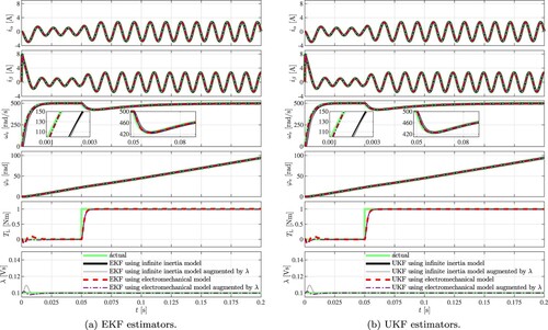
Table 1. Comparison of RMSE values for simulation using nominal parameters.

Estimator	RMSE of
	$i_{\alpha }$ [A]	$i_{\text{β}}$ [A]	${\omega }_e$ [rad/s]	${\phi }_e$ [rad]	$T_L$ [Nm]	λ [Vs]
EKF using infinite inertia model	$2.2927\cdot {10}^{-4}$	$1.9085\cdot {10}^{-3}$	11.0953	0.0503	–	–
EKF using infinite inertia model augmented by λ	$2.3625\cdot {10}^{-4}$	$1.9078\cdot {10}^{-3}$	12.2471	0.0530	–	$1.1378\cdot {10}^{-3}$
EKF using electromechanical model	$5.0767\cdot {10}^{-5}$	$1.8859\cdot {10}^{-3}$	1.7352	0.0499	0.0878	–
EKF using electromechanical model augmented by λ	$4.8545\cdot {10}^{-5}$	$1.8856\cdot {10}^{-3}$	2.3189	0.0517	0.0861	$4.3916\cdot {10}^{-4}$
UKF using infinite inertia model	$2.2663\cdot {10}^{-4}$	$1.9085\cdot {10}^{-3}$	11.0597	0.0499	–	–
UKF using infinite inertia model augmented by λ	$2.3473\cdot {10}^{-4}$	$1.9078\cdot {10}^{-3}$	12.1948	0.0518	–	$1.1407\cdot {10}^{-3}$
UKF using electromechanical model	$4.5641\cdot {10}^{-5}$	$1.8857\cdot {10}^{-3}$	1.6951	0.0492	0.0880	–
UKF using electromechanical model augmented by λ	$4.5579\cdot {10}^{-5}$	$1.8855\cdot {10}^{-3}$	2.3187	0.0505	0.0861	$3.1030\cdot {10}^{-4}$

In the second simulation, the PM flux linkage sensitivity of the estimators is investigated. Therefore, the parameter λ is reduced by 20% in the PMSM simulation model. Thus, λ parameter is inaccurate in estimators using conventional infinite inertia or electromechanical models, and the initial value of λ is incorrect in estimators using augmented models. The results are shown in Figure 2 and Table 2. Conventional estimators without λ estimation show increased position estimation error and very significant velocity estimation error. In addition, load estimation is very poor for estimators using the conventional electromechanical model. On the other hand, EKF and UKF with PM flux linkage estimation are almost insensitive to the λ uncertainty. Since the estimated value of λ converges relatively quickly to the actual value, all variables are accurately estimated when using the augmented models.

Figure 2. Performance of the position sensorless state estimators in the case of 20% detuned λ. (a) EKF estimators and (b) UKF estimators.

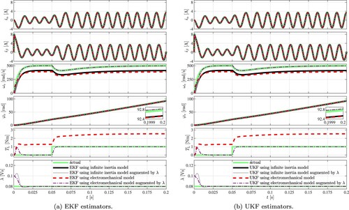
Table 2. Comparison of RMSE values for simulation using 20% detuned λ.

Estimator	RMSE of
	$i_{\alpha }$ [A]	$i_{\text{β}}$ [A]	${\omega }_e$ [rad/s]	${\phi }_e$ [rad]	$T_L$ [Nm]	λ [Vs]
EKF based on infinite inertia model	$2.5260\cdot {10}^{-3}$	$3.1596\cdot {10}^{-3}$	83.9020	0.2366	–	–
EKF based on infinite inertia model augmented by λ	$2.6196\cdot {10}^{-4}$	$1.9094\cdot {10}^{-3}$	17.1699	0.0619	–	$4.1420\cdot {10}^{-3}$
EKF based on electromechanical model	$2.5468\cdot {10}^{-3}$	$3.1719\cdot {10}^{-3}$	103.9686	0.2488	1.3855	–
EKF based on electromechanical model augmented by λ	$8.5668\cdot {10}^{-5}$	$1.8896\cdot {10}^{-3}$	5.1097	0.0544	0.1465	$2.9644\cdot {10}^{-3}$
UKF based on infinite inertia model	$2.5147\cdot {10}^{-3}$	$3.1507\cdot {10}^{-3}$	83.5885	0.2372	–	–
UKF based on infinite inertia model augmented by λ	$2.6008\cdot {10}^{-4}$	$1.9090\cdot {10}^{-3}$	17.1012	0.0603	–	$4.1598\cdot {10}^{-3}$
UKF based on electromechanical model	$2.5352\cdot {10}^{-3}$	$3.1625\cdot {10}^{-3}$	103.6145	0.2498	1.3791	–
UKF based on electromechanical model augmented by λ	$8.2951\cdot {10}^{-5}$	$1.8892\cdot {10}^{-3}$	4.9176	0.0519	0.1450	$2.9878\cdot {10}^{-3}$

The estimators with λ estimation show much better performance than the conventional estimators in case of PM flux linkage mismatch. However, the estimation error can also be caused by variations in other parameters. To analyze the impact of stator inductance and resistance uncertainty, two additional simulations are performed. First, parameter L is reduced by 20% and the results are shown in Figure 3 and Table 3. It can be seen that 20% difference in L has very little effect on the performance of the estimators. In contrast, the accuracy of speed and load estimation decreases if R differs by 20%, as shown in Figure 4 and Table 4. However, the error of estimators using augmented models is smaller than that of conventional estimators. In addition to electrical parameters, electromechanical models also include mechanical parameters D and J. However, these parameters are not used in infinite inertia models. Therefore, the effect of variations in mechanical parameters is not investigated in this study.

Figure 3. Performance of the position sensorless state estimators in the case of 20% detuned L. (a) EKF estimators, (b) UKF estimators.

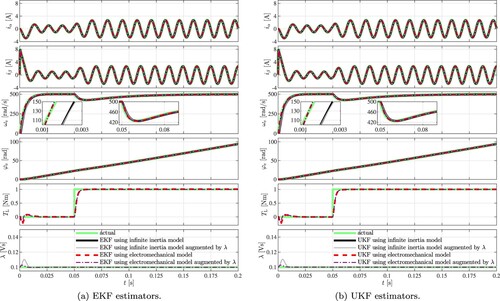
Figure 4. Performance of the position sensorless state estimators in the case of 20% detuned R. (a) EKF estimators, (b) UKF estimators.

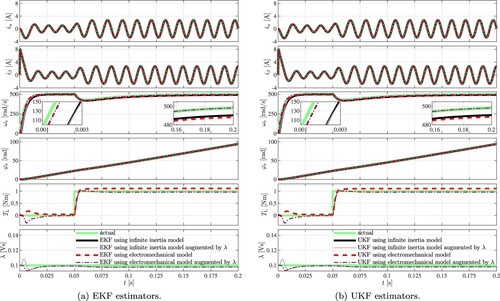
Table 3. Comparison of RMSE values for simulation using 20% detuned L.

Estimator	RMSE of
	$i_{\alpha }$ [A]	$i_{\text{β}}$ [A]	${\omega }_e$ [rad/s]	${\phi }_e$ [rad]	$T_L$ [Nm]	λ [Vs]
EKF based on infinite inertia model	$2.0465\cdot {10}^{-4}$	$1.9728\cdot {10}^{-3}$	10.5148	0.0370	–	–
EKF based on infinite inertia model augmented by λ	$2.1154\cdot {10}^{-4}$	$1.9720\cdot {10}^{-3}$	12.0462	0.0399	–	$1.3016\cdot {10}^{-3}$
EKF based on electromechanical model	$3.4070\cdot {10}^{-5}$	$1.9483\cdot {10}^{-3}$	2.2051	0.0364	0.0869	–
EKF based on electromechanical model augmented by λ	$2.9263\cdot {10}^{-5}$	$1.9482\cdot {10}^{-3}$	1.8168	0.0380	0.0855	$3.7081\cdot {10}^{-4}$
UKF based on infinite inertia model	$2.0225\cdot {10}^{-4}$	$1.9728\cdot {10}^{-3}$	10.4784	0.0366	–	–
UKF based on infinite inertia model augmented by λ	$2.1013\cdot {10}^{-4}$	$1.9721\cdot {10}^{-3}$	11.9950	0.0387	–	$1.3302\cdot {10}^{-3}$
UKF based on electromechanical model	$2.9813\cdot {10}^{-5}$	$1.9482\cdot {10}^{-3}$	2.1867	0.0358	0.0872	–
UKF based on electromechanical model augmented by λ	$2.8667\cdot {10}^{-5}$	$1.9481\cdot {10}^{-3}$	1.8589	0.0364	0.0857	$3.5988\cdot {10}^{-4}$

Table 4. Comparison of RMSE values for simulation using 20% detuned R.

Estimator	RMSE of
	$i_{\alpha }$ [A]	$i_{\text{β}}$ [A]	${\omega }_e$ [rad/s]	${\phi }_e$ [rad]	$T_L$ [Nm]	λ [Vs]
EKF based on infinite inertia model	$3.5678\cdot {10}^{-4}$	$1.9270\cdot {10}^{-3}$	15.6556	0.0368	–	–
EKF based on infinite inertia model augmented by λ	$2.8013\cdot {10}^{-4}$	$1.9124\cdot {10}^{-3}$	14.4513	0.0559	–	$2.4121\cdot {10}^{-3}$
EKF based on electromechanical model	$2.4889\cdot {10}^{-4}$	$1.9071\cdot {10}^{-3}$	9.1324	0.0324	0.1268	–
EKF based on electromechanical model augmented by λ	$9.6137\cdot {10}^{-5}$	$1.8916\cdot {10}^{-3}$	4.9279	0.0534	0.1027	$2.4139\cdot {10}^{-3}$
UKF based on infinite inertia model	$3.4883\cdot {10}^{-4}$	$1.9259\cdot {10}^{-3}$	15.5055	0.0364	–	–
UKF based on infinite inertia model augmented by λ	$2.7851\cdot {10}^{-4}$	$1.9122\cdot {10}^{-3}$	14.3878	0.0547	–	$2.2370\cdot {10}^{-3}$
UKF based on electromechanical model	$2.3859\cdot {10}^{-4}$	$1.9057\cdot {10}^{-3}$	8.7648	0.0317	0.1227	–
UKF based on electromechanical model augmented by λ	$9.2214\cdot {10}^{-5}$	$1.8914\cdot {10}^{-3}$	4.8101	0.0517	0.1015	$2.1890\cdot {10}^{-3}$

In summary, conventional EKF and UKF estimators work properly if the parameters of the PMSM are known accurately. Although the error in speed estimation is smaller during acceleration if the model used includes the equation of motion. However, all conventional estimators are highly sensitive to the uncertainty in the PM flux linkage. In contrast, estimators using augmented models are almost insensitive to PM flux linkage variation. The estimation accuracy depends mainly on the model used, but the Kalman filter algorithm used has practically no effect. The performance using the different models is summarized in Table 5.

Table 5. Comparison of estimation performances using different state-space models.

Applied model	Estimation of
	Rotor velocity	Rotor position	Load torque	PM flux linkage
Infinite inertia model	Moderate during acceleration, sensitive to λ and slightly sensitive to R variations	Slightly sensitive to λ variation	–	–
Infinite inertia model augmented by λ	Moderate during acceleration, but accurate at steady state	Accurate	–	Accurate
Electromechanical model	Sensitive to λ and slightly sensitive to R variations	Slightly sensitive to λ variation	Sensitive to λ and slightly sensitive to R variations	–
Electromechanical model augmented by λ	Accurate	Accurate	Accurate	Accurate

It is important to highlight that the observability conditions of the models used in the estimators were fulfilled in the simulations, when the rotor speed was not zero. Since the observability conditions are fulfilled, the models are locally weakly observable and the state vectors can be fully reconstructed from the measurements. If a model is unobservable, then the state-space model has several different solutions, so not all estimated state variables follow the actual values when they change. For this reason, it is important to analyze and ensure observability.

According to the simulation results, there is no difference between the performance of the EKF and UKF estimators when using the same model. However, it is well known that the UKF has higher computational burden than the EKF, since the application of the UT requires multiple evaluations of the nonlinear function. To compare the computational burdens, a target computer with Intel Core i5-2500 @ 3.3 GHz processor is used with the software tools provided by MATLAB R2018b Simulink Real-Time toolbox. Using Embedded Coder, target codes are generated for each estimator implemented in MATLAB/Simulink. Then the target codes are executed one by one in real-time on the target computer, while measuring the average task execution time using software tool Task Execution Time Monitor. For real-time execution of estimators, the sampling time is set to 100 μs. The average task execution times for each estimator are shown in Table 6. In case of the infinite inertia model with 4 state variables, the computational time of the UKF is approximately 14% higher than that of the EKF. If the model used for estimation has 5 state variables, the difference is 18%, and for 6 state variables it is about 19%. Since EKF and UKF provide the same accuracy, but UKF requires slightly more computational effort, the use of EKF estimators are recommended for PMSM drives.

Table 6. Comparison of the average execution time of the estimators.

Estimator	Average execution time [s]
EKF using infinite inertia model	$3.0425\cdot {10}^{-6}$
EKF using infinite inertia model augmented by λ	$3.2481\cdot {10}^{-6}$
EKF using electromechanical model	$3.2655\cdot {10}^{-6}$
EKF using electromechanical model augmented by λ	$3.5391\cdot {10}^{-6}$
UKF using infinite inertia model	$3.4783\cdot {10}^{-6}$
UKF using infinite inertia model augmented by λ	$3.8283\cdot {10}^{-6}$
UKF using electromechanical model	$3.8373\cdot {10}^{-6}$
UKF using electromechanical model augmented by λ	$4.2098\cdot {10}^{-6}$

5. Conclusions

In this study, novel position sensorless EKF and UKF state estimators have been presented for surface-mounted PMSM. The proposed estimators use augmented models in which the PM flux linkage is a state variable, so they can also estimate the PM flux linkage. For the models used for state estimation, a detailed observability study has been presented. To compare the estimation performances, numerical simulations have been carried out. The results showed that the proposed estimators are almost insensitive to the uncertainty in the PM flux linkage, unlike the conventional estimators using infinite inertia or electromechanical models. Since there is no difference between the performance of the EKF and UKF when using the same model, and the EKF has less computation time, EKF estimators are recommended for position sensorless PMSM drives.

Disclosure statement

No potential conflict of interest was reported by the author(s).

Additional information

Funding

Supported by the ÚNKP-23-4-II-SZE-73 New National Excellence Program of the Ministry for Culture and Innovation from the source of the National Research, Development and Innovation Fund.

References

- Zhu ZQ, Liang D, Liu K. Online parameter estimation for permanent magnet synchronous machines: An overview. IEEE Access. 2021;9:59059–59084. doi: 10.1109/ACCESS.2021.3072959
- Li S, Xia C, Zhou X. Disturbance rejection control method for permanent magnet synchronous motor speed-regulation system. Mechatronics. 2012;22(6):706–714. doi: 10.1016/j.mechatronics.2012.02.007
- Lu E, Li W, Wang S, et al. Disturbance rejection control for PMSM using integral sliding mode based composite nonlinear feedback control with load observer. ISA Trans. 2021;116:203–217. doi: 10.1016/j.isatra.2021.01.008
- Jankowska K, Petro V, Dybkowski M, et al. The application of a sliding mode observer in a speed sensor fault tolerant PMSM drive system. IEEE Access. 2023;11:130899–130908. doi: 10.1109/ACCESS.2023.3335121
- Amirouche E, Iffouzar K, Houari A, et al. Improved control strategy of dual star permanent magnet synchronous generator based tidal turbine system using sensorless field oriented control and direct power control techniques. Energy Sources A. 2021;43:1–22. doi: 10.1080/15567036.2021.1902429
- Zafari Y, Shoja-Majidabad S. Sensorless fault-tolerant control of five-phase IPMSMs via model reference adaptive systems. Automatika. 2020;61(4):564–573. doi: 10.1080/00051144.2020.1797349
- Solsona J, Valla M, Muravchik C. Nonlinear control of a permanent magnet synchronous motor with disturbance torque estimation. IEEE Trans Energy Convers. 2000;15(2):163–168. doi: 10.1109/60.866994
- Po-ngam S, Sangwongwanich S. Stability and dynamic performance improvement of adaptive full-order observers for sensorless PMSM drive. IEEE Trans Power Electron. 2012;27(2):588–600. doi: 10.1109/TPEL.2011.2153212
- Kyslan K, Petro V, Bober P, et al. A comparative study and optimization of switching functions for sliding-mode observer in sensorless control of PMSM. Energies. 2022;15(7):1–17. doi: 10.3390/en15072689
- Zuo Y, Lai C, Iyer KLV. A review of sliding mode observer based sensorless control methods for PMSM drive. IEEE Trans Power Electron. 2023;38(9):11352–11367. doi: 10.1109/TPEL.2023.3287828
- Bolognani S, Oboe R, Zigliotto M. Sensorless full-digital PMSM drive with EKF estimation of speed and rotor position. IEEE Trans Ind Electron. 1999;46(1):184–191. doi: 10.1109/41.744410
- Chan TF, Borsje P, Wang W. Application of unscented Kalman filter to sensorless permanent-magnet synchronous motor drive.Miami, USA.IEEE International Electric Machines and Drives Conference (IEMDC). 2009. p. 631–638, doi: 10.1109/IEMDC.2009.5075272.
- Xiao D, Nalakath S, Filho SR, et al. Universal full-speed sensorless control scheme for interior permanent magnet synchronous motors. IEEE Trans Power Electron. 2021;36(4):4723–4737. doi: 10.1109/TPEL.63
- Wang G, Valla M, Solsona J. Position sensorless permanent magnet synchronous machine drives – A review. IEEE Trans Ind Electron. 2020;67(7):5830–5842. doi: 10.1109/TIE.41
- Vaclavek P, Blaha P, Herman I. AC drive observability analysis. IEEE Trans Ind Electron. 2013;60(8):3047–3059. doi: 10.1109/TIE.2012.2203775
- Zerdali E, Rivera M, Wheeler P, et al. Speed-sensorless predictive direct speed control for PMSM drives Florianopolis, Brazil 17th Brazilian Power Electronics Conference – 8th IEEE International Conference on Southern Power Electronics Conference (COBEP/SPEC) 2023 p. 1–6, doi: 10.1109/SPEC56436.2023.10408131.
- Koteich M, Maloum A, Duc G, et al. Permanent magnet synchronous drives observability analysis for motion-sensorless control Sydney, Australia IEEE Symposium on Sensorless Control for Electrical Drives (SLED) 2015 p. 56–63, doi: 10.1109/SLED.2015.7339264.
- Inoue Y, Kawaguchi Y, Morimoto S, et al. Performance improvement of sensorless IPMSM drives in a low-speed region using online parameter identification. IEEE Trans Ind Appl. 2011;47(2):798–804. doi: 10.1109/TIA.2010.2101994
- Han YS, Choi JS, Kim YS. Sensorless PMSM drive with a sliding mode control based adaptive speed and stator resistance estimator. IEEE Trans Magn. 2000;36(5):3588–3591. doi: 10.1109/20.908786
- Gopinath GR, Shyama PD. Speed and position sensorless control of interior permanent magnet synchronous motor using square-root cubature Kalman filter with joint parameter estimation.Trivandrum, India.IEEE International Conference on Power Electronics, Drives and Energy Systems (PEDES).2016. p. 1867–1871, doi: 10.1109/PEDES.2016.7914540.
- Zhang X, Zhang L, Zhang Y. Model predictive current control for PMSM drives with parameter robustness improvement. IEEE Trans Power Electron. 2019;34(2):1645–1657. doi: 10.1109/TPEL.2018.2835835
- Shi Y, Sun K, Huang L, et al. Online identification of permanent magnet flux based on extended Kalman filter for IPMSM drive with position sensorless control. IEEE Trans Ind Electron. 2012;59(11):4169–4178. doi: 10.1109/TIE.2011.2168792
- Zerdali E, Wheeler P. Speed-sensorless finite control set model predictive control of PMSM with permanent magnet flux linkage estimation.Izmir, Turkey.2nd Global Power, Energy and Communication Conference (GPECOM).2020. p. 114–119, doi: 10.1109/GPECOM49333.2020.9247943.
- Horváth K. Load torque and permanent magnet flux linkage estimation of surface-mounted PMSM by using unscented Kalman filter.The High Tatras, Slovakia International Conference on Electrical Drives and Power Electronics (EDPE)2023. p. 402–409, doi: 10.1109/EDPE58625.2023.10274042.
- Julier S, Uhlmann J. Unscented filtering and nonlinear estimation. Proc IEEE. 2004;92(3):401–422. doi: 10.1109/JPROC.2003.823141
- Yildiz R, Barut M, Zerdali E. A comprehensive comparison of extended and unscented Kalman filters for speed-sensorless control applications of induction motors. IEEE Trans Ind Inf. 2020;16(10):6423–6432. doi: 10.1109/TII.9424
- Horváth K, Fodor D. Low speed operation of sensorless estimators for induction machines using extended, unscented and cubature Kalman filter techniques. The High Tatras, Slovakia. International Conference on Electrical Drives and Power Electronics (EDPE). 2019. p. 279–285, doi: 10.1109/EDPE.2019.8883936.