Full article: The relaxed gradient based iterative algorithm for solving the generalized coupled complex conjugate and transpose Sylvester matrix equations

Formulae display: $MathJax Logo$ ?Mathematical formulae have been encoded as MathML and are displayed in this HTML version using MathJax in order to improve their display. Uncheck the box to turn MathJax off. This feature requires Javascript. Click on a formula to zoom.

Abstract

Inspired by the idea of Ma et al. (Journal of the Franklin Institute, 2018), we adopt relaxation technique and introduce relaxation factors into the gradient based iterative (GI) algorithm, and the relaxed based iterative (RGI) algorithm is established to solve the generalized coupled complex conjugate and transpose Sylvester matrix equations. By applying the real representation and straighten operation, we contain the sufficient and necessary condition for convergence of the RGI method. In order to effectively utilize this algorithm, we further derive the optimal convergence parameter and some related conclusions. Moreover, to overcome the high dimension calculation problem, a sufficient condition for convergence with less computational complexity is determined. Finally, numerical examples are reported to demonstrate the availability and superiority of the constructed iterative algorithm.

Keywords:

1. Introduction

Solving matrix equations is one of the research focuses of computational mathematics [Citation1–4]. The Sylvester matrix equation is an important type of matrix equations, which has a wide range of applications in control and system theory, pole assignment, model reduction and so further [Citation5–7]. Therefore, finding feasible and effective algorithms for the Sylvester matrix equation has important theoretical significance and practical application value.

In this paper, we aim to find the solution of the generalized coupled complex conjugate and transpose Sylvester matrix equations (1) $\begin{aligned} \sum_{j = 1}^{q} (A_{ij} Y_{j} B_{ij} + C_{ij} \bar{Y_{j}} D_{ij} \\ + E_{ij} Y_{j}^{T} F_{ij} + G_{ij} Y_{j}^{H} H_{ij}) = M_{i}, i \in I [1, p], \end{aligned}$ (1) where $A_{ij}, C_{ij} \in C^{m_{i} \times r_{j}}$ , $B_{ij}, D_{ij} \in C^{s_{j} \times n_{i}}$ , $E_{ij}, G_{ij} \in C^{m_{i} \times s_{j}}$ , $F_{ij}, H_{ij} \in C^{r_{j} \times n_{i}}$ , $M_{i} \in C^{m_{i} \times n_{i}}$ , $i \in I [1, p]$ , $i \in I [1, q]$ are the known matrices and $Y_{j} \in C^{r_{j} \times s_{j}}$ are unknown matrices to be solved. Equation (Equation1(1) $\begin{aligned} \sum_{j = 1}^{q} (A_{ij} Y_{j} B_{ij} + C_{ij} \bar{Y_{j}} D_{ij} \\ + E_{ij} Y_{j}^{T} F_{ij} + G_{ij} Y_{j}^{H} H_{ij}) = M_{i}, i \in I [1, p], \end{aligned}$ (1) ) is involved in both science and engineering. Besides, its form includes many other special matrix equations, such as complex conjugate Sylvester matrix equations, complex transpose Sylvester matrix equations and complex conjugate and transpose Sylvester matrix equations [Citation8–10]. Therefore, it is meaningful to research efficient methods for solving Equation (Equation1(1) $\begin{aligned} \sum_{j = 1}^{q} (A_{ij} Y_{j} B_{ij} + C_{ij} \bar{Y_{j}} D_{ij} \\ + E_{ij} Y_{j}^{T} F_{ij} + G_{ij} Y_{j}^{H} H_{ij}) = M_{i}, i \in I [1, p], \end{aligned}$ (1) ).

At present, the methods for solving the Sylvester matrix equation mainly include direct methods and iterative methods. However, when solving high-dimensional matrix equations, the direct methods may lead to lengthy computation time. In order to efficiently solve these matrix equations, we prefer to apply iterative methods. In the past few decades, many scholars are devoted to establishing iterative methods to solve various types of Sylvester matrix equations [Citation7,Citation11–14].

From the previous works [Citation15,Citation16], we know that it is difficult to calculate the exact solution of matrix equations, which consumes large computing costs. In the field of systems and control, calculating approximate solutions is sufficient. So iterative solutions have been widely concerned by researchers, and many researchers paid attention to iterative methods and got excellent results. Ding and Chen developed various iterative algorithms to solve Ax = b, AXB = F and other Sylvester matrix equations [Citation17–19]. Subsequently, many effective iterative methods were proposed. In [Citation10], the least squares based iterative method has been applied to find the solutions of the Sylvester transpose matrix equation $AXB + C X^{T} D = F$ . Xie and Ding constructed the gradient based iterative (GI) methods for the matrix equations AXB + CXD = F [Citation9]. Wu et al. also investigated the GI method for solving the Sylvester conjugate matrix equation $AXB + C \bar{X} D = F$ [Citation20]. Owing to the availability of the GI algorithm, the GI algorithm has been extended to solve general Sylvester matrix equations by researchers. For instance, Wu et al. proposed the GI algorithm to find the solution of coupled Sylvester-conjugate matrix equations [Citation21] (2) $\sum_{i = 1}^{l} (A_{ij} X_{j} B_{ij} + C_{ij} {\bar{X}}_{j} D_{ij}) = F_{i}, i \in I [1, s],$ (2) where $A_{ij}, C_{ij} \in C^{m_{i} \times r_{j}}$ , $B_{ij}, D_{ij} \in C^{t_{j} \times n_{i}}$ , $F_{ij} \in C^{m_{i} \times n_{i}}$ ( $i \in I [1, s]$ , $j \in I [1, l])$ are the known matrices. Song et al. applied the GI method to the coupled Sylvester-transpose matrix equations [Citation22] (3) $\sum_{i = 1}^{l} (A_{ij} X_{j} B_{ij} + C_{ij} X_{j}^{T} D_{ij}) = F_{i}, i \in I [1, s],$ (3) where $A_{ij} \in R^{m_{i} \times r_{j}}$ , $C_{ij} \in R^{m_{i} \times t_{j}}$ , $B_{ij} \in C^{t_{j} \times n_{i}}$ , $D_{ij} \in C^{r_{j} \times n_{i}}$ , ( $i \in I [1, s]$ , $j \in I [1, l]$ ) are the known matrices. The above two matrix equations are important types of matrix equations, which are frequently involved in the fields of systems and control. Not only that, they are also the generalized forms of matrix equations in [Citation10,Citation20], respectively. The convergence properties and the optimal convergence parameters of the GI algorithm for Equations (Equation2(2) $\sum_{i = 1}^{l} (A_{ij} X_{j} B_{ij} + C_{ij} {\bar{X}}_{j} D_{ij}) = F_{i}, i \in I [1, s],$ (2) ) and (Equation3(3) $\sum_{i = 1}^{l} (A_{ij} X_{j} B_{ij} + C_{ij} X_{j}^{T} D_{ij}) = F_{i}, i \in I [1, s],$ (3) ) have been investigated.

Subsequently, Beik et al. proposed the GI algorithm for solving the generalized coupled Sylvester-transpose and conjugate matrix equations [Citation23] (4) $\begin{aligned} T_{v} (X) & = \sum_{i = 1}^{p} (\sum_{μ = 1}^{s_{1}} A_{viμ} X_{i} B_{viμ} + \sum_{μ = 1}^{s_{2}} C_{viμ} X_{i}^{T} D_{viμ} \\ + \sum_{μ = 1}^{s_{3}} M_{viμ} \bar{X_{i}} N_{viμ} + \sum_{μ = 1}^{s_{4}} H_{viμ} X_{i}^{H} G_{viμ}) \\ = F_{v}, \end{aligned}$ (4) where $A_{viμ}, B_{viμ}, C_{viμ}, D_{viμ}, M_{viμ}, N_{viμ}, H_{viμ}, G_{viμ}, F_{v} (v = 1, 2, \dots, N)$ are known matrices with proper dimensions. The form of the above matrix equations is quite general. When p and $s_{1}, s_{2}, s_{3}, s_{4}$ , are taken to be some special values, Equation (Equation4(4) $\begin{aligned} T_{v} (X) & = \sum_{i = 1}^{p} (\sum_{μ = 1}^{s_{1}} A_{viμ} X_{i} B_{viμ} + \sum_{μ = 1}^{s_{2}} C_{viμ} X_{i}^{T} D_{viμ} \\ + \sum_{μ = 1}^{s_{3}} M_{viμ} \bar{X_{i}} N_{viμ} + \sum_{μ = 1}^{s_{4}} H_{viμ} X_{i}^{H} G_{viμ}) \\ = F_{v}, \end{aligned}$ (4) ) can be transformed into other matrix equations.

Except for the above classical Sylvester matrix equations, the GI algorithm has also been applied to solve periodic matrix equations [Citation24,Citation25]. Li et al. established the GI method for the forward periodic Sylvester matrix equations and backward forward periodic Sylvester matrix equations [Citation25] (5) $A_{i} X_{i} B_{i} + C_{i} X_{i + 1} D_{i} = F_{i}, i \in I [1, γ],$ (5) and (6) $A_{i} X_{i + 1} B_{i} + C_{i} X_{i} D_{i} = F_{i}, i \in I [1, γ],$ (6) where $A_{i}, B_{i}, C_{i}, D_{i}, F_{i} \in R^{n \times n}$ are the known matrices. In theory, Li et al. proposed the sufficient and necessary conditions for the convergence of the GI algorithm. Numerical experiments have also showed the effectiveness of the GI algorithm.

Although the theory of the GI algorithm has been systematically proposed by researchers, this algorithm still has some drawbacks. In [Citation26], Fan et al. pointed out that the GI algorithm costs large computation time and storage space when encountering ill-posed problems. In order to further optimize the convergence performance of the GI algorithm, the relaxed gradient based iterative (RGI) algorithm has been proposed by introducing the relaxed factor to adjust the weight of the iteration sequences. Niu et al. developed the RGI algorithm to solve the Sylvester matrix equations [Citation27]. Numerical experiments have shown that relaxation techniques can effectively reduce computation time and storage space, and improve the convergence rate of the GI algorithm.

Due to the superiority of the RGI algorithm, many scholars have extended this algorithm to solve more general matrix equations. Recently, in [Citation28,Citation29], Huang et al. applied the RGI algorithm to solve coupled Sylvester-conjugate matrix equation (Equation2(2) $\sum_{i = 1}^{l} (A_{ij} X_{j} B_{ij} + C_{ij} {\bar{X}}_{j} D_{ij}) = F_{i}, i \in I [1, s],$ (2) ) and coupled Sylvester-transpose matrix equation (Equation3(3) $\sum_{i = 1}^{l} (A_{ij} X_{j} B_{ij} + C_{ij} X_{j}^{T} D_{ij}) = F_{i}, i \in I [1, s],$ (3) ). And the experiments results illustrate that the convergence rate of the RGI algorithm is faster than the GI one. Then Wang et al. consider the solution of the complex conjugate and transpose matrix equations (7) $A_{1} X B_{1} + A_{2} \bar{X} B_{2} + A_{3} X^{T} B_{3} + A_{4} X^{H} B_{4} = E,$ (7) where $A_{i}$ , $B_{i}$ , $E \in C^{n \times n}$ ( $i \in I [1, 4]$ ) are the known matrices. By introducing relaxation factors and applying the hierarchical identification principle [Citation30], Wang et al. presented the RGI method to solve Equation (Equation7(7) $A_{1} X B_{1} + A_{2} \bar{X} B_{2} + A_{3} X^{T} B_{3} + A_{4} X^{H} B_{4} = E,$ (7) ). However, Wang et al. didn't discuss the generalized form of Equation (Equation7(7) $A_{1} X B_{1} + A_{2} \bar{X} B_{2} + A_{3} X^{T} B_{3} + A_{4} X^{H} B_{4} = E,$ (7) ). Based on the ideas of [Citation30], we extend the RGI algorithm to the generalized coupled complex conjugate and transpose Sylvester matrix equations.

Inspired by the idea of [Citation28], we construct the RGI algorithm for solving Equation (Equation1(1) $\begin{aligned} \sum_{j = 1}^{q} (A_{ij} Y_{j} B_{ij} + C_{ij} \bar{Y_{j}} D_{ij} \\ + E_{ij} Y_{j}^{T} F_{ij} + G_{ij} Y_{j}^{H} H_{ij}) = M_{i}, i \in I [1, p], \end{aligned}$ (1) ). Its form can be specific written as

(8) ${\begin{cases} \sum_{j = 1}^{q} A_{1 j} Y_{j} B_{1 j} + \sum_{j = 1}^{q} C_{1 j} \bar{Y_{j}} D_{1 j} \\ + \sum_{j = 1}^{q} E_{1 j} Y_{j}^{T} F_{1 j} + \sum_{j = 1}^{q} G_{1 j} Y_{j}^{H} H_{1 j} = M_{1}, \\ \sum_{j = 1}^{q} A_{2 j} Y_{j} B_{2 j} + \sum_{j = 1}^{q} C_{2 j} \bar{Y_{j}} D_{2 j} \\ + \sum_{j = 1}^{q} E_{2 j} Y_{j}^{T} F_{2 j} + \sum_{j = 1}^{q} G_{2 j} Y_{j}^{H} H_{2 j} = M_{2}, \\ ⋮ \\ \sum_{j = 1}^{q} A_{pj} Y_{j} B_{pj} + \sum_{j = 1}^{q} C_{pj} \bar{Y_{j}} D_{pj} \\ + \sum_{j = 1}^{q} E_{pj} Y_{j}^{T} F_{pj} + \sum_{j = 1}^{q} G_{pj} Y_{j}^{H} H_{p} = M_{p} . \end{cases}$ (8) The form of the above matrix equations is quite general, which contains several classic Sylverster matrix equations. Especially, Equations (Equation2(2) $\sum_{i = 1}^{l} (A_{ij} X_{j} B_{ij} + C_{ij} {\bar{X}}_{j} D_{ij}) = F_{i}, i \in I [1, s],$ (2) )–(Equation3(3) $\sum_{i = 1}^{l} (A_{ij} X_{j} B_{ij} + C_{ij} X_{j}^{T} D_{ij}) = F_{i}, i \in I [1, s],$ (3) ) are special cases of Equation (Equation1(1) $\begin{aligned} \sum_{j = 1}^{q} (A_{ij} Y_{j} B_{ij} + C_{ij} \bar{Y_{j}} D_{ij} \\ + E_{ij} Y_{j}^{T} F_{ij} + G_{ij} Y_{j}^{H} H_{ij}) = M_{i}, i \in I [1, p], \end{aligned}$ (1) ). If i = j = p = q = 1, Equation (Equation1(1) $\begin{aligned} \sum_{j = 1}^{q} (A_{ij} Y_{j} B_{ij} + C_{ij} \bar{Y_{j}} D_{ij} \\ + E_{ij} Y_{j}^{T} F_{ij} + G_{ij} Y_{j}^{H} H_{ij}) = M_{i}, i \in I [1, p], \end{aligned}$ (1) ) will reduce to Equation (Equation7(7) $A_{1} X B_{1} + A_{2} \bar{X} B_{2} + A_{3} X^{T} B_{3} + A_{4} X^{H} B_{4} = E,$ (7) ). Therefore, finding faster algorithms to solve Equation (Equation1(1) $\begin{aligned} \sum_{j = 1}^{q} (A_{ij} Y_{j} B_{ij} + C_{ij} \bar{Y_{j}} D_{ij} \\ + E_{ij} Y_{j}^{T} F_{ij} + G_{ij} Y_{j}^{H} H_{ij}) = M_{i}, i \in I [1, p], \end{aligned}$ (1) ) is of great significance.

To accelerate convergence rate of the GI algorithm for Equation (Equation1(1) $\begin{aligned} \sum_{j = 1}^{q} (A_{ij} Y_{j} B_{ij} + C_{ij} \bar{Y_{j}} D_{ij} \\ + E_{ij} Y_{j}^{T} F_{ij} + G_{ij} Y_{j}^{H} H_{ij}) = M_{i}, i \in I [1, p], \end{aligned}$ (1) ), we combine relaxation technology with hierarchical identification principle, and we derive the relaxed gradient based iterative (RGI) algorithm to solve Equation (Equation1(1) $\begin{aligned} \sum_{j = 1}^{q} (A_{ij} Y_{j} B_{ij} + C_{ij} \bar{Y_{j}} D_{ij} \\ + E_{ij} Y_{j}^{T} F_{ij} + G_{ij} Y_{j}^{H} H_{ij}) = M_{i}, i \in I [1, p], \end{aligned}$ (1) ). This principle regards the unknown matrix as the system parameter matrix to be solved, then it builds a recursive formula to approach the unknown solution [Citation27,Citation28,Citation30,Citation31]. Furthermore, we can effectively control the weight of the iteration sequence by introducing relaxation factors. In theory, we exploit the real representation and the straightening operator to prove the convergence properties of the constructed algorithm. Meanwhile, the sufficient and necessary condition for convergence is presented. Finally, numerical experiments further demonstrate the effectiveness and superiority of the RGI algorithm. The main motivation and contribution of this paper are summarized as follows:

In order to accelerate the convergence rate of the GI algorithm [Citation23], we combine the GI algorithm with relaxation technique. By introducing l relaxation factors, we construct the RGI algorithm for Equation (Equation1(1) $\begin{aligned} \sum_{j = 1}^{q} (A_{ij} Y_{j} B_{ij} + C_{ij} \bar{Y_{j}} D_{ij} \\ + E_{ij} Y_{j}^{T} F_{ij} + G_{ij} Y_{j}^{H} H_{ij}) = M_{i}, i \in I [1, p], \end{aligned}$ (1) ). Due to that Equation (Equation1(1) $\begin{aligned} \sum_{j = 1}^{q} (A_{ij} Y_{j} B_{ij} + C_{ij} \bar{Y_{j}} D_{ij} \\ + E_{ij} Y_{j}^{T} F_{ij} + G_{ij} Y_{j}^{H} H_{ij}) = M_{i}, i \in I [1, p], \end{aligned}$ (1) ) extremely is general, the algorithm constructed in this paper is also more general. It is meaningful to promote the development of the field of solving matrix equations.
To optimize convergence theory, we utilize real representation and straighten operation as tool, and present the sufficient and necessary condition for convergence of the RGI method. To overcome high-dimensional computing problems, the sufficient condition for convergence and some related results are proposed. Besides, we use numerical experiments to fully demonstrate the effectiveness and superiority of the RGI algorithm.

The remainder of this paper is structured as follows. In Section 2, we list several useful notations and definitions. Moreover, we construct the relaxed gradient based iterative (RGI) algorithm to find the iterative solution of Equation (Equation1(1) $\begin{aligned} \sum_{j = 1}^{q} (A_{ij} Y_{j} B_{ij} + C_{ij} \bar{Y_{j}} D_{ij} \\ + E_{ij} Y_{j}^{T} F_{ij} + G_{ij} Y_{j}^{H} H_{ij}) = M_{i}, i \in I [1, p], \end{aligned}$ (1) ) in Section 3. In Section 4, we deduce the convergence properties of the proposed method, including the sufficient and necessary condition for convergence, the optimal convergence factor and the related corollary. In Section 5, two numerical experiments are reported to validate the superior of convergence for the new algorithm. In the end, Section 6 proposes the some conclusions.

2. Preliminaries

For the sake of convenience, we provide several main notations and lemmas which are used throughout this paper. The set of $m \times n$ complex matrix is denoted by $C^{m \times n}$ . For $A \in C^{m \times n}$ , there are some related notations as follows:

$\bar{A}$ indicates the conjugate of the matrix A;
$A^{T}$ represents the transpose of the matrix A;
$A^{H}$ stands for the conjugate transpose of the matrix A;
$σ_{max} (A)$ stands for the maximal singular of the matrix A;
$σ_{min} (A)$ stands for the minimal singular of the matrix A;
$cond (A) = σ_{max} (A) / σ_{min} (A)$ is defined as the condition number of A;
$λ_{max} (A)$ represents the maximal eigenvalue of the matrix A;
$λ_{min} (A)$ indicates the minimal eigenvalue of the matrix A;
$∥ A ∥_{2}$ is defined as the the spectral norm of the matrix A.
$∥ A ∥$ indicates the Frobenius norm of the matrix A.
$ρ (A)$ represents the spectral radius of the matrix A;

Then, some significant definitions and lemmas are listed below.

Definition 2.1

[Citation28]

Let $A \in C^{m \times n}$ , then A can be uniquely expressed as $A = A_{1} + i A_{2}$ with $A_{1}, A_{2} \in R^{m \times n}$ . $A^{▽}$ denotes the real representation of a complex matrix A (9) $A^{▽} = (\begin{array}{cc} A_{1} & - A_{2} \\ A_{2} & A_{1} \end{array}) \in R^{2 m \times 2 n} .$ (9)

Definition 2.2

[Citation32]

For two matrices $A = (a_{ij}) \in C^{m \times n}$ , $B = (b_{ij}) \in C^{k \times l}$ , the Kronecker product is defined as (10) $A \otimes B = (\begin{array}{cccc} a_{11} B & a_{12} B & \dots & a_{1 n} B \\ a_{21} B & a_{22} B & \dots & a_{2 n} B \\ ⋮ & ⋮ & ⋮ \\ a_{m 1} B & a_{m 2} B & \dots & a_{mn} B \end{array}) .$ (10)

Definition 2.3

[Citation28]

Let $e_{in}$ denote an n-dimensional column vector which has 1 in the ith position and 0's elsewhere. The vec-permutation matrix $P_{mn}$ can be defined as (11) $P_{mn} := (\begin{array}{l} I_{m} \otimes e_{1 n}^{T} \\ I_{m} \otimes e_{2 n}^{T} \\ ⋮ \\ I_{m} \otimes e_{nn}^{T} \end{array}) .$ (11) If $X, A \in C^{m \times n}$ and $B \in C^{p \times q}$ , we have (12) $P_{mn} P_{mn} = I_{mn}, P_{mn}^{T} = P_{mn}^{- 1} = P_{mn},$ (12) and (13) $\begin{aligned} B \otimes A & = P_{mp}^{T} (A \otimes B) P_{nq}, \\ (A \otimes B) P_{nq} & = P_{mp} (B \otimes A) . \end{aligned}$ (13)

Next, we review several lemmas which are used to prove the convergence property.

Lemma 2.1

[Citation33]

If $A \in C^{m \times n}$ , $B \in C^{s \times t}$ , $X \in C^{n \times s}$ , then (14) $\begin{aligned} vec (ABC) & = (C^{T} \otimes A) vec (B), \end{aligned}$ (14) (15) $\begin{aligned} (A \otimes B) (C \otimes D) & = (AC) \otimes (BD) . \end{aligned}$ (15)

Lemma 2.2

[Citation29]

For two matrices A and B, it has (16) $‖ A \otimes B ‖_{2} = ‖ A ‖_{2} ‖ B ‖_{2} .$ (16)

Lemma 2.3

[Citation28]

For $A \in C^{m \times r}$ , $B \in C^{s \times n}$ , $F \in C^{m \times n}$ , if the matrix equation AXB = F has unique solution, then the iterative sequences ${X (k)}$ converges to the exact solution $X^{*}$ for any initial matrix $X (0)$ by the following algorithm (17) $X (k + 1) = X (k) + μ A^{H} (F - AX (k) B) B^{H},$ (17) and the algorithm is convergent if and only if (18) $0 < μ < \frac{2}{‖ A ‖_{2}^{2} ‖ B ‖_{2}^{2}} .$ (18) Meanwhile, the optimal convergence factor is (19) $μ_{0} = \frac{2}{\begin{array}{l} λ_{max} (A^{H} A) λ_{max} (B^{H} B) \\ + λ_{min} (A^{H} A) λ_{min} (B^{H} B) \end{array}} .$ (19)

Proof.

Define error matrix $\tilde{X} (k) = X (k) - X^{*} .$ According to the expression (Equation17(17) $X (k + 1) = X (k) + μ A^{H} (F - AX (k) B) B^{H},$ (17) ), it has $\tilde{X} (k + 1) = \tilde{X} (k) - μ A^{H} A \tilde{X} (k) B B^{H} .$ Let $Z (k) = A \tilde{X} (k) B$ , utilizing the properties of matrix Frobenius norm, Lemmas 2.1 and 2.2, it follows that $\begin{aligned} ‖ \tilde{X} (k + 1) ‖^{2} \\ = ‖ \tilde{X} (k) ‖^{2} - μtr (B^{H} {\tilde{X}}^{H} (k) A^{H} Z (k)) \\ - μtr (Z^{H} (k) A \tilde{X} (k) B) + μ^{2} ‖ A^{H} Z (k) B^{H} ‖^{2} \\ \leq ‖ \tilde{X} (k) ‖^{2} - μtr (Z^{H} (k) Z (k)) - μtr (Z^{H} (k) Z (k)) \\ + μ^{2} ‖ (\bar{B} \otimes A^{H}) vec (Z (k)) ‖^{2} \\ = ‖ \tilde{X} (k) ‖^{2} - μ (2 - μ ‖ \bar{B} \otimes A^{H} ‖_{2}^{2}) ‖ Z (k) ‖^{2} \\ = ‖ \tilde{X} (k) ‖^{2} - μ (2 - μ ‖ A ‖_{2}^{2} ‖ B ‖_{2}^{2}) ‖ Z (k) ‖^{2} . \end{aligned}$ Repeatedly applying the relationship of the above expression leads to $\begin{aligned} ‖ \tilde{X} (k + 1) ‖^{2} \\ \leq ‖ \tilde{X} (k - 1) ‖^{2} - μ (2 - μ ‖ A ‖_{2}^{2} ‖ B ‖_{2}^{2}) (‖ Z (k) ‖^{2} \\ + ‖ Z (k - 1) ‖^{2}) \\ \leq ‖ \tilde{X} (0) ‖^{2} - μ (2 - μ ‖ A ‖_{2}^{2} ‖ B ‖_{2}^{2}) (\sum_{i = 0}^{k} ‖ Z (i) ‖^{2}) . \end{aligned}$ If the convergence parameter μ is selected to satisfy $0 < μ < \frac{2}{‖ A ‖_{2}^{2} ‖ B ‖_{2}^{2}},$ the following inequality holds $0 < μ (2 - μ ‖ A ‖_{2}^{2} ‖ B ‖_{2}^{2}) \sum_{i = 0}^{\infty} ‖ Z (i) ‖^{2} \leq ‖ \tilde{X} (0) ‖^{2} .$ This means that $lim_{i \to \infty} ‖ Z (i) ‖^{2} = 0$ . Due to that the matrix equation AXB = F has unique solution, then it has $lim_{k \to \infty} \tilde{X} (k) = 0$ . The proof of Equation (Equation18(18) $0 < μ < \frac{2}{‖ A ‖_{2}^{2} ‖ B ‖_{2}^{2}} .$ (18) ) is completed.

Taking the vec-operator of both sides of the expression (Equation17(17) $X (k + 1) = X (k) + μ A^{H} (F - AX (k) B) B^{H},$ (17) ) and applying Lemma 2.2, it can get $vec (\tilde{X} (k + 1)) = (I - μB B^{H} \otimes A^{H} A) vec (\tilde{X} (k)) .$ The above equation implies that $I - μB B^{H} \otimes A^{H} A$ is the iterative matrix of the algorithm. Thus, the optimal convergence parameter satisfies the following equation $\begin{aligned} min max {| 1 - μ λ_{1} (B B^{H} \otimes A^{H} A) |, \dots, \\ 1 - μ λ_{sm} (B B^{H} \otimes A^{H} A) |} \\ = min max {| 1 - μ λ_{max} (B B^{H} \otimes A^{H} A) |, \\ | 1 - μ λ_{min} (B B^{H} \otimes A^{H} A) |}, \end{aligned}$ which means that $| 1 - μ λ_{max} (B B^{H} \otimes A^{H} A) | = | 1 - μ λ_{min} (B B^{H} \otimes A^{H} A) |$ has a non-trivial solution. By simple deductions, Expression (Equation19(19) $μ_{0} = \frac{2}{\begin{array}{l} λ_{max} (A^{H} A) λ_{max} (B^{H} B) \\ + λ_{min} (A^{H} A) λ_{min} (B^{H} B) \end{array}} .$ (19) ) can be obtained.

Lemma 2.4

[Citation28]

The properties of real representation $(.)^{▽}$ are as follows:

For two complex matrices $A \in C^{m \times n}$ , $B \in C^{n \times r}$ , then (20) $\begin{aligned} (AB)^{▽} & = A^{▽} B^{▽}, (A^{T})^{▽} = E_{n} (A^{▽})^{T} E_{m}, \\ (A^{H})^{▽} & = (A^{▽})^{T}, (\bar{A})^{▽} = E_{m} A^{▽} E_{n} . \end{aligned}$ (20) Here, unitary matrices $E_{n}$ is defined as (21) $E_{n} = (\begin{array}{cc} 0 & I_{n} \\ I_{n} & 0 \end{array}) .$ (21) Furthermore, based on the definition of matrix Frobenius norm and real representation, then (22) $\begin{aligned} ‖ A^{▽} ‖^{2} & = 2 ‖ A ‖^{2}, \end{aligned}$ (22) (23) $\begin{aligned} ‖ A^{▽} ‖_{2} & = ‖ A ‖_{2} . \end{aligned}$ (23)

Lemma 2.5

[Citation29]

If $m_{i}, i \in I [1, n]$ are any given positive number, denote the maximum and minimum values of $m_{i}$ as $m_{max} = {max}_{1 \leq i \leq n} m_{i}$ and $m_{min} = {min}_{1 \leq i \leq n} m_{i}$ , respectively. It has (24) $min_{0 < μ < \frac{2}{m_{max}}} max_{1 \leq i \leq n} | 1 - μ m_{i} | = \frac{m_{max} - m_{min}}{m_{max} + m_{min}},$ (24) then, the optimal convergence parameter μ is selected as $μ_{opt} = \frac{2}{m_{max} + m_{min}} .$

Proof.

Build function $y = {max}_{1 \leq i \leq n} | 1 - μ m_{i} |$ , and then Equation (Equation24(24) $min_{0 < μ < \frac{2}{m_{max}}} max_{1 \leq i \leq n} | 1 - μ m_{i} | = \frac{m_{max} - m_{min}}{m_{max} + m_{min}},$ (24) ) has been obtained by drawing graph in [Citation29]. Besides, $| 1 - μ m_{i} | < 1$ if and only if $0 < u < \frac{2}{m_{max}}$ . The optimal convergence factor μ satisfies $\begin{aligned} min max {| 1 - μ m_{1} |, | 1 - μ m_{2} |, \dots, | 1 - μ m_{n} |} \\ = min max {| 1 - μ m_{1} |, | 1 - μ m_{n} |} . \end{aligned}$ The above equation indicates that $| 1 - μ m_{} | = | 1 - μ m_{n} |$ , that is, $- 1 + μ m_{1} = 1 - μ m_{n}$ . By simple calculations, it has $μ_{opt} = \frac{2}{m_{1} + m_{n}} = \frac{2}{m_{max} + m_{min}} .$ Thus, the proof is completed.

3. The relaxed gradient-based iterative algorithm

In this section, we mainly propose the relaxed gradient based iterative (RGI) algorithm to solve the generalized coupled complex conjugate and transpose matrix equation. The main idea of this algorithm is to use the hierarchical identification principle to divide Equation (Equation1(1) $\begin{aligned} \sum_{j = 1}^{q} (A_{ij} Y_{j} B_{ij} + C_{ij} \bar{Y_{j}} D_{ij} \\ + E_{ij} Y_{j}^{T} F_{ij} + G_{ij} Y_{j}^{H} H_{ij}) = M_{i}, i \in I [1, p], \end{aligned}$ (1) ) into several subsystems. The unknown matrixes $Y_{j}$ are regarded as the identified parameters matrices. Meanwhile, we construct intermediate matrices and adopt an average strategy. Then, the relaxation factors $ω_{l}$ , $l \in I [1, q]$ are introduced, which are utilized to adjust the weights of matrix schemes. The construction process of the RGI algorithm is as follows.

Firstly, define the following intermediate matrices, $i \in I [1, p]$ , $l \in I [1, q]$ , (25) $\begin{aligned} Π_{il} & = M_{i} - \sum_{j = 1}^{q} (A_{ij} Y_{j} B_{ij} + C_{ij} \bar{Y_{j}} D_{ij} + E_{ij} Y_{j}^{T} F_{ij} \\ + G_{ij} Y_{j}^{H} H_{ij}) + A_{il} Y_{l} B_{il}, \end{aligned}$ (25) (26) $\begin{aligned} Υ_{il} & = \bar{\begin{array}{l} M_{i} - \sum_{j = 1}^{q} (A_{ij} Y_{j} B_{ij} + C_{ij} \bar{Y_{j}} D_{ij} + E_{ij} Y_{j}^{T} F_{ij} \\ + G_{ij} Y_{j}^{H} H_{ij}) + C_{il} {\bar{Y}}_{l} D_{il}, \end{array}} \end{aligned}$ (26) (27) $\begin{aligned} Φ_{il} & = (M_{i} - \sum_{j = 1}^{q} (A_{ij} Y_{j} B_{ij} + C_{ij} \bar{Y_{j}} D_{ij} + E_{ij} Y_{j}^{T} F_{ij} \\ + G_{ij} Y_{j}^{H} H_{ij}) + E_{il} Y_{l}^{T} F_{il})^{T}, \end{aligned}$ (27) (28) $\begin{aligned} Ψ_{il} & = (M_{i} - \sum_{j = 1}^{q} (A_{ij} Y_{j} B_{ij} + C_{ij} \bar{Y_{j}} D_{ij} + E_{ij} Y_{j}^{T} F_{ij} \\ + G_{ij} Y_{j}^{H} H_{ij}) + G_{il} Y_{l}^{H} H_{il})^{H} . \end{aligned}$ (28) From the expression of Equation (Equation1(1) $\begin{aligned} \sum_{j = 1}^{q} (A_{ij} Y_{j} B_{ij} + C_{ij} \bar{Y_{j}} D_{ij} \\ + E_{ij} Y_{j}^{T} F_{ij} + G_{ij} Y_{j}^{H} H_{ij}) = M_{i}, i \in I [1, p], \end{aligned}$ (1) ), some subsystems are given below, $i \in I [1, p]$ , $l \in I [1, q]$ , (29) $\begin{aligned} A_{il} Y_{l} B_{il} & = Π_{il}, \end{aligned}$ (29) (30) $\begin{aligned} \bar{C_{il}} Y_{l} \bar{D_{il}} & = Υ_{il}, \end{aligned}$ (30) (31) $\begin{aligned} F_{il}^{T} Y_{l} E_{il}^{T} & = Φ_{il}, \end{aligned}$ (31) (32) $\begin{aligned} H_{il}^{H} Y_{l} G_{il}^{H} & = Ψ_{il} . \end{aligned}$ (32) According to the above fictitious subsystems and Lemma 2.3, we can put forward the iterative schemes as follows, $i \in I [1, p]$ , $l \in I [1, q]$ , (33) $\begin{aligned} Y_{l}^{1, i} (k + 1) & = Y_{l}^{1, i} (k) + μ A_{il}^{H} [Π_{il} - A_{il} Y_{l}^{1, i} (k) B_{il}] B_{il}^{H}, \end{aligned}$ (33) (34) $\begin{aligned} Y_{l}^{2, i} (k + 1) & = Y_{l}^{2, i} (k) + μ C_{il}^{T} [Υ_{il} - \bar{C_{il}} Y_{l}^{2, i} (k) \bar{D_{il}}] D_{il}^{T}, \end{aligned}$ (34) (35) $\begin{aligned} Y_{l}^{3, i} (k + 1) & = Y_{l}^{3, i} (k) + μ \bar{F_{il}} [Φ_{il} - F_{il}^{T} Y_{l}^{3, i} (k) E_{il}^{T}] \bar{E_{il}}, \end{aligned}$ (35) (36) $\begin{aligned} Y_{l}^{4, i} (k + 1) & = Y_{l}^{4, i} (k) + μ H_{il} [Ψ_{il} - H_{il}^{H} Y_{l}^{4, i} (k) G_{il}^{H}] G_{il} . \end{aligned}$ (36) For the sake of convenience, we provide the following notations, $s \in I [1, 4]$ , (37) $\begin{aligned} Γ_{ij}^{s, i} (k) & = \sum_{j = 1}^{q} (A_{ij} Y_{j}^{s, i} (k) B_{ij} + C_{ij} \bar{Y_{j}^{s, i} (k)} D_{ij} \\ + E_{ij} Y_{j}^{s, i} (k)^{T} F_{ij} + G_{ij} Y_{j}^{s, i} (k)^{H} H_{ij}) . \end{aligned}$ (37) Combining Equations (Equation25(25) $\begin{aligned} Π_{il} & = M_{i} - \sum_{j = 1}^{q} (A_{ij} Y_{j} B_{ij} + C_{ij} \bar{Y_{j}} D_{ij} + E_{ij} Y_{j}^{T} F_{ij} \\ + G_{ij} Y_{j}^{H} H_{ij}) + A_{il} Y_{l} B_{il}, \end{aligned}$ (25) )–(Equation28(28) $\begin{aligned} Ψ_{il} & = (M_{i} - \sum_{j = 1}^{q} (A_{ij} Y_{j} B_{ij} + C_{ij} \bar{Y_{j}} D_{ij} + E_{ij} Y_{j}^{T} F_{ij} \\ + G_{ij} Y_{j}^{H} H_{ij}) + G_{il} Y_{l}^{H} H_{il})^{H} . \end{aligned}$ (28) ) with Equations(Equation33(33) $\begin{aligned} Y_{l}^{1, i} (k + 1) & = Y_{l}^{1, i} (k) + μ A_{il}^{H} [Π_{il} - A_{il} Y_{l}^{1, i} (k) B_{il}] B_{il}^{H}, \end{aligned}$ (33) )–(Equation36(36) $\begin{aligned} Y_{l}^{4, i} (k + 1) & = Y_{l}^{4, i} (k) + μ H_{il} [Ψ_{il} - H_{il}^{H} Y_{l}^{4, i} (k) G_{il}^{H}] G_{il} . \end{aligned}$ (36) ) and utilizing the hierarchical identification principle, the recursive systems are established. Due to that the unknown matrices $Y_{j}$ are included in the expressions, we replace $Y_{j}$ in (Equation25(25) $\begin{aligned} Π_{il} & = M_{i} - \sum_{j = 1}^{q} (A_{ij} Y_{j} B_{ij} + C_{ij} \bar{Y_{j}} D_{ij} + E_{ij} Y_{j}^{T} F_{ij} \\ + G_{ij} Y_{j}^{H} H_{ij}) + A_{il} Y_{l} B_{il}, \end{aligned}$ (25) )–(Equation28(28) $\begin{aligned} Ψ_{il} & = (M_{i} - \sum_{j = 1}^{q} (A_{ij} Y_{j} B_{ij} + C_{ij} \bar{Y_{j}} D_{ij} + E_{ij} Y_{j}^{T} F_{ij} \\ + G_{ij} Y_{j}^{H} H_{ij}) + G_{il} Y_{l}^{H} H_{il})^{H} . \end{aligned}$ (28) ) with $Y_{j}^{1, i} (k), Y_{j}^{2, i} (k), Y_{j}^{3, i} (k), Y_{j}^{4, i} (k)$ , respectively. Therefore, the following expressions are given, $i \in I [1, p]$ , $l \in I [1, q]$ , (38) $\begin{aligned} X_{l}^{1, i} (k + 1) & = X_{l}^{1, i} (k) + μ A_{il}^{H} [M_{i} - \sum_{j = 1}^{q} Γ_{ij}^{1, i} (k)] B_{il}^{H}, \end{aligned}$ (38) (39) $\begin{aligned} X_{l}^{2, i} (k + 1) & = X_{l}^{2, i} (k) + μ C_{il}^{T} \bar{[M_{i} - \sum_{j = 1}^{q} Γ_{ij}^{2, i} (k)]} D_{il}^{T}, \end{aligned}$ (39) (40) $\begin{aligned} X_{l}^{3, i} (k + 1) & = X_{l}^{3, i} (k) + μ \bar{F_{il}} {[M_{i} - \sum_{j = 1}^{q} Γ_{ij}^{3, i} (k)]}^{T} \bar{E_{il}}, \end{aligned}$ (40) (41) $\begin{aligned} X_{l}^{4, i} (k + 1) & = X_{l}^{4, i} (k) + μ H_{il} {[M_{i} - \sum_{j = 1}^{q} Γ_{ij}^{4, i} (k)]}^{H} G_{il} . \end{aligned}$ (41) Then, by taking the average value of $Y_{j}^{1, i} (k), Y_{j}^{2, i} (k), Y_{j}^{3, i} (k)$ and $Y_{j}^{4, i} (k)$ , for $i \in I [1, p]$ we have $\begin{aligned} Y_{l}^{'} (k + 1) & = Y_{l}^{'} (k) + \frac{μ}{p} \sum_{i = 1}^{p} A_{il}^{H} \\ \times [M_{i} - \sum_{j = 1}^{q} (A_{ij} Y_{j}^{'} (k) B_{ij} + C_{ij} \bar{Y_{j}^{'} (k)} D_{ij} \\ + E_{ij} Y_{j}^{'} (k)^{T} F_{ij} + G_{ij} Y_{j}^{'} (k)^{H} H_{ij})] B_{il}^{H}, \\ Y_{l}^{′′} (k + 1) & = Y_{l}^{′′} (k) + \frac{μ}{p} \sum_{i = 1}^{p} C_{il}^{T} \\ \bar{\begin{array}{l} [M_{i} - \sum_{j = 1}^{q} (A_{ij} Y_{j}^{′′} (k) B_{ij} \\ + C_{ij} \bar{Y_{j}^{′′} (k)} D_{ij} + E_{ij} Y_{j}^{′′} (k)^{T} F_{ij} \\ + G_{ij} Y_{j}^{′′} (k)^{H} H_{ij})] \end{array}} D_{il}^{T}, \\ \overset{ˇ}{Y_{l}} (k + 1) & = \overset{ˇ}{Y_{l}} (k) + \frac{μ}{p} \sum_{i = 1}^{p} \bar{F_{il}} \\ \times [M_{i} - \sum_{j = 1}^{q} (A_{ij} \overset{ˇ}{Y_{j}} (k) B_{ij} + C_{ij} \bar{\overset{ˇ}{Y_{j}} (k)} D_{ij} \\ + E_{ij} \overset{ˇ}{Y_{j}} (k)^{T} F_{ij} + G_{ij} \overset{ˇ}{Y_{j}} (k)^{H} H_{ij})]^{T} \bar{E_{il}}, \\ \overset{´}{Y_{l}} (k + 1) & = \overset{´}{Y_{l}} (k) + \frac{μ}{p} \sum_{i = 1}^{p} H_{il} \\ \times [M_{i} - \sum_{j = 1}^{q} (A_{ij} \overset{´}{Y_{j}} (k) B_{ij} + C_{ij} \bar{\overset{´}{Y_{j}} (k)} D_{ij} \\ + E_{ij} \overset{´}{Y_{j}} (k)^{T} F_{ij} + G_{ij} \overset{´}{Y_{j}} (k)^{H} H_{ij})]^{H} G_{il} . \end{aligned}$ Inspire by the idea of the RGI method in [Citation28], we introduce the relaxation factors $ω_{l}$ ( $l \in I [1, q]$ ) into the above recursive systems. Based on the previous analysis process, the relaxed gradient-based iterative (RGI) algorithm for Equation (Equation1(1) $\begin{aligned} \sum_{j = 1}^{q} (A_{ij} Y_{j} B_{ij} + C_{ij} \bar{Y_{j}} D_{ij} \\ + E_{ij} Y_{j}^{T} F_{ij} + G_{ij} Y_{j}^{H} H_{ij}) = M_{i}, i \in I [1, p], \end{aligned}$ (1) ) is presented as follows.

In the RGI algorithm μ indicates the convergence parameter. The relaxation factors $ω_{l}$ ( $l \in I [1, q]$ ) are used to control the weight of iterative sequences, and it can effectively improve the convergence rate of the GI method. In particular, if the relaxed factors are selected as $ω_{l} = \frac{1}{2}$ for all l, Algorithm 1 will reduce to the GI algorithm [Citation23]. Besides, Algorithm 1 with $ω_{l} = \frac{1}{2}$ and p = q = i = j = 1 will change into the iterative method in [Citation30]. Compared with the RGI algorithm in [Citation28], the new algorithm is more general which includes many kind of iterative formulas.

In what follows, the convergence properties of the RGI method are analysed below. At the same time, we also provide the detailed proof of convergence theory.

4. Convergence analysis of the RGI algorithm

The section presents the sufficient and necessary condition for convergence of the RGI algorithm. Furthermore, to overcome the high-dimensional calculation problem of the iterative matrix, we further discuss the sufficient condition for convergence.

Theorem 4.1

Assume that the generalized coupled complex conjugate and transpose matrix Equation (Equation1(1) $\begin{aligned} \sum_{j = 1}^{q} (A_{ij} Y_{j} B_{ij} + C_{ij} \bar{Y_{j}} D_{ij} \\ + E_{ij} Y_{j}^{T} F_{ij} + G_{ij} Y_{j}^{H} H_{ij}) = M_{i}, i \in I [1, p], \end{aligned}$ (1) ) has a unique solution, then the iterative sequences $Y_{l} (k)$ $l \in I [1, q]$ converge to the exact solution $Y_{l}^{*}$ by the RGI algorithm for any initial matrices $Y_{l} (0)$ for all $l \in I [1, q]$ if and only if the convergence factor μ is selected to satisfy (42) $0 < μ < \frac{2}{‖ Q M^{\frac{1}{2}} ‖_{2}^{2}},$ (42) where (43) $\begin{aligned} M & = (\begin{array}{cc} \frac{1}{4} ω_{1} (1 - ω_{1}) I_{4 s_{1} r_{1}} & 0 \\ 0 & \frac{1}{4} ω_{2} (1 - ω_{2}) I_{4 s_{2} r_{2}} \\ ⋮ & ⋮ \\ 0 & 0 \end{array} \\ \begin{array}{cc} \dots & 0 \\ \dots & 0 \\ ⋱ & ⋮ \\ \dots & \frac{1}{4} ω_{q} (1 - ω_{q}) I_{4 s_{q} r_{q}} \end{array}), \end{aligned}$ (43) (44) $\begin{aligned} Q & = (\begin{array}{cccc} Q_{11} & Q_{12} & \dots & Q_{1 q} \\ Q_{21} & Q_{22} & \dots & Q_{2 q} \\ ⋮ & ⋮ & ⋱ & ⋮ \\ Q_{p 1} & Q_{p 2} & \dots & Q_{pq} \end{array}), \end{aligned}$ (44) (45) $\begin{aligned} Q_{ij} & = (B_{ij}^{▽})^{T} \otimes (A_{ij}^{▽}) + (D_{ij}^{▽})^{T} E_{sj} \otimes (C_{ij}^{▽}) E_{rj} \\ + ((F_{ij}^{▽})^{T} E_{rj} \otimes (E_{ij}^{▽}) E_{sj}) P_{4 r_{j} s_{j}} \\ + ((H_{ij}^{▽})^{T} \otimes (G_{ij}^{▽})) P_{4 r_{j} s_{j}}, i \in I [1, p], \\ l \in I [1, q] . \end{aligned}$ (45)

Proof.

Denote (46) $\begin{aligned} {\tilde{Y}}_{l}^{(1)} (k) & = Y_{l}^{(1)} (k) - Y_{l}^{*}, {\tilde{Y}}_{l}^{(2)} (k) = Y_{l}^{(2)} (k) - Y_{l}^{*}, \\ {\tilde{Y}}_{l}^{(3)} (k) & = Y_{l}^{(3)} (k) - Y_{l}^{*}, \\ {\tilde{Y}}_{l}^{(4)} (k) & = Y_{l}^{(4)} (k) - Y_{l}^{*}, \\ {\tilde{Y}}_{l} (k) & = Y_{l} (k) - Y_{l}^{*}, l \in I [1, q] . \end{aligned}$ (46) To facilitate our statement, the expressions of $Z_{i} (k) (i \in I [1, p])$ are defined as follows (47) $\begin{aligned} Z_{i} (k) & = \sum_{j = 1}^{q} (A_{ij} {\tilde{Y}}_{j} (k) B_{ij} + C_{ij} {\bar{\tilde{Y}}}_{j} (k) D_{ij} + E_{ij} {\tilde{Y}}_{j} (k)^{T} F_{ij} \\ + G_{ij} {\tilde{Y}}_{j} (k)^{H} H_{ij}) . \end{aligned}$ (47) From the definition of error matrices and the expression of $Y_{l}^{(1)} (k + 1)$ in the RGI algorithm, we derive that for $l \in I [1, q]$ (48) $\begin{aligned} {\tilde{Y}}_{l}^{(1)} (k + 1) = Y_{l}^{(1)} (k + 1) - Y_{l}^{*} \\ = {\tilde{Y}}_{l}^{(1)} (k) - \frac{1}{2} μ ω_{l} \sum_{i = 1}^{p} A_{il}^{H} \\ \times [\sum_{j = 1}^{q} (A_{ij} {\tilde{Y}}_{j} (k) B_{ij} + C_{ij} {\bar{\tilde{Y}}}_{j} (k) D_{ij} \\ + E_{ij} {\tilde{Y}}_{j} (k)^{T} F_{ij} + G_{ij} {\tilde{Y}}_{j} (k)^{H} H_{ij}] B_{il}^{H} \\ = {\tilde{Y}}_{l}^{(1)} (k) - \frac{1}{2} μ ω_{l} \sum_{i = 1}^{p} A_{il}^{H} Z_{i} (k) B_{il}^{H} . \end{aligned}$ (48) It follows from the expression of $Y_{l}^{(2)} (k + 1)$ in the RGI method that (49) $\begin{aligned} {\tilde{Y}}_{l}^{(2)} (k + 1) = Y_{l}^{(2)} (k + 1) - Y_{l}^{*} \\ = {\tilde{Y}}_{l}^{(2)} (k) - \frac{1}{2} μ ω_{l} \sum_{i = 1}^{p} C_{il}^{T} \\ \times [\begin{matrix} \bar{\begin{array}{l} \sum_{j = 1}^{q} (A_{ij} {\tilde{Y}}_{j} (k) B_{ij} + C_{ij} {\bar{\tilde{Y}}}_{j} (k) D_{ij} \\ + E_{ij} {\tilde{Y}}_{j} (k)^{T} F_{ij} + G_{ij} {\tilde{Y}}_{j} (k)^{H} H_{ij} \end{array}} \end{matrix}] D_{il}^{T} \\ = {\tilde{Y}}_{l}^{(2)} (k) - \frac{1}{2} μ ω_{l} \sum_{i = 1}^{p} C_{il}^{T} \bar{Z_{i} (k)} D_{il}^{T} . \end{aligned}$ (49) By the expression of $Y_{l}^{(3)} (k + 1)$ in Algorithm 1, for $l \in I [1, q]$ one has (50) $\begin{aligned} {\tilde{Y}}_{l}^{(3)} (k + 1) = Y_{l}^{(3)} (k + 1) - Y_{l}^{*} \\ = {\tilde{Y}}_{l}^{(3)} (k) - \frac{1}{2} μ (1 - ω_{l}) \sum_{i = 1}^{p} \bar{F_{il}} \\ \times [\sum_{j = 1}^{q} (A_{ij} {\tilde{Y}}_{j} (k) B_{ij} + C_{ij} {\bar{\tilde{Y}}}_{j} (k) D_{ij} \\ {+ E_{ij} {\tilde{Y}}_{j} (k)^{T} F_{ij} + G_{ij} {\tilde{Y}}_{j} (k)^{H} H_{ij}]}^{T} \bar{E_{il}} \\ = {\tilde{Y}}_{l}^{(3)} (k) - \frac{1}{2} μ (1 - ω_{l}) \sum_{i = 1}^{p} \bar{F_{il}} Z_{i} (k)^{T} \bar{E_{il}} . \end{aligned}$ (50) It follows from the expression of $Y_{l}^{(4)} (k + 1)$ in Algorithm 1 that for $l \in I [1, q]$ (51) $\begin{aligned} {\tilde{Y}}_{l}^{(4)} (k + 1) = Y_{l}^{(4)} (k + 1) - Y_{l}^{*} \\ = {\tilde{Y}}_{l}^{(4)} (k) - \frac{1}{2} μ (1 - ω_{l}) \sum_{i = 1}^{p} H_{il} \\ \times [\sum_{j = 1}^{q} (A_{ij} {\tilde{Y}}_{j} (k) B_{ij} + C_{ij} {\bar{\tilde{Y}}}_{j} (k) D_{ij} + E_{ij} {\tilde{Y}}_{j} (k)^{T} F_{ij} \\ {+ G_{ij} {\tilde{Y}}_{j} (k)^{H} H_{ij}]}^{H} G_{il} \\ = {\tilde{Y}}_{l}^{(4)} (k) - \frac{1}{2} μ (1 - ω_{l}) \sum_{i = 1}^{p} H_{il} Z_{i} (k)^{H} G_{il} . \end{aligned}$ (51) Combing (Equation48(48) $\begin{aligned} {\tilde{Y}}_{l}^{(1)} (k + 1) = Y_{l}^{(1)} (k + 1) - Y_{l}^{*} \\ = {\tilde{Y}}_{l}^{(1)} (k) - \frac{1}{2} μ ω_{l} \sum_{i = 1}^{p} A_{il}^{H} \\ \times [\sum_{j = 1}^{q} (A_{ij} {\tilde{Y}}_{j} (k) B_{ij} + C_{ij} {\bar{\tilde{Y}}}_{j} (k) D_{ij} \\ + E_{ij} {\tilde{Y}}_{j} (k)^{T} F_{ij} + G_{ij} {\tilde{Y}}_{j} (k)^{H} H_{ij}] B_{il}^{H} \\ = {\tilde{Y}}_{l}^{(1)} (k) - \frac{1}{2} μ ω_{l} \sum_{i = 1}^{p} A_{il}^{H} Z_{i} (k) B_{il}^{H} . \end{aligned}$ (48) )–(Equation51(51) $\begin{aligned} {\tilde{Y}}_{l}^{(4)} (k + 1) = Y_{l}^{(4)} (k + 1) - Y_{l}^{*} \\ = {\tilde{Y}}_{l}^{(4)} (k) - \frac{1}{2} μ (1 - ω_{l}) \sum_{i = 1}^{p} H_{il} \\ \times [\sum_{j = 1}^{q} (A_{ij} {\tilde{Y}}_{j} (k) B_{ij} + C_{ij} {\bar{\tilde{Y}}}_{j} (k) D_{ij} + E_{ij} {\tilde{Y}}_{j} (k)^{T} F_{ij} \\ {+ G_{ij} {\tilde{Y}}_{j} (k)^{H} H_{ij}]}^{H} G_{il} \\ = {\tilde{Y}}_{l}^{(4)} (k) - \frac{1}{2} μ (1 - ω_{l}) \sum_{i = 1}^{p} H_{il} Z_{i} (k)^{H} G_{il} . \end{aligned}$ (51) ) with Line 5 of the RGI algorithm leads to (52) $\begin{aligned} {\tilde{Y}}_{l} (k + 1) & = Y_{l} (k + 1) - Y_{l}^{*} \\ = \frac{1}{2} (1 - ω_{l}) Y_{l}^{(1)} (k + 1) \\ + \frac{1}{2} (1 - ω_{l}) Y_{l}^{(2)} (k + 1) \\ + \frac{1}{2} ω_{l} Y_{l}^{(3)} (k + 1) \\ + \frac{1}{2} ω_{l} Y_{l}^{(4)} (k + 1) - Y_{l}^{*} \\ = \frac{1}{2} (1 - ω_{l}) {\tilde{Y}}_{l}^{(1)} (k + 1) \\ + \frac{1}{2} (1 - ω_{l}) {\tilde{Y}}_{l}^{(2)} (k + 1) \\ + \frac{1}{2} ω_{l} {\tilde{Y}}_{l}^{(3)} (k + 1) \\ + \frac{1}{2} ω_{l} {\tilde{Y}}_{l}^{(4)} (k + 1) \\ = {\tilde{Y}}_{l} (k) - \frac{1}{4} μ ω_{l} (1 - ω_{l}) \sum_{i = 1}^{p} (A_{il}^{H} Z_{i} (k) B_{il}^{H} \\ + C_{il}^{T} \bar{Z_{i} (k)} D_{il}^{T} + \bar{F_{il}} Z_{i} (k)^{T} \bar{E_{il}} \\ + H_{il} Z_{i} (k)^{H} G_{il}) . \end{aligned}$ (52) According to Lemma 2.4, taking the real representation on both sides of (Equation52(52) $\begin{aligned} {\tilde{Y}}_{l} (k + 1) & = Y_{l} (k + 1) - Y_{l}^{*} \\ = \frac{1}{2} (1 - ω_{l}) Y_{l}^{(1)} (k + 1) \\ + \frac{1}{2} (1 - ω_{l}) Y_{l}^{(2)} (k + 1) \\ + \frac{1}{2} ω_{l} Y_{l}^{(3)} (k + 1) \\ + \frac{1}{2} ω_{l} Y_{l}^{(4)} (k + 1) - Y_{l}^{*} \\ = \frac{1}{2} (1 - ω_{l}) {\tilde{Y}}_{l}^{(1)} (k + 1) \\ + \frac{1}{2} (1 - ω_{l}) {\tilde{Y}}_{l}^{(2)} (k + 1) \\ + \frac{1}{2} ω_{l} {\tilde{Y}}_{l}^{(3)} (k + 1) \\ + \frac{1}{2} ω_{l} {\tilde{Y}}_{l}^{(4)} (k + 1) \\ = {\tilde{Y}}_{l} (k) - \frac{1}{4} μ ω_{l} (1 - ω_{l}) \sum_{i = 1}^{p} (A_{il}^{H} Z_{i} (k) B_{il}^{H} \\ + C_{il}^{T} \bar{Z_{i} (k)} D_{il}^{T} + \bar{F_{il}} Z_{i} (k)^{T} \bar{E_{il}} \\ + H_{il} Z_{i} (k)^{H} G_{il}) . \end{aligned}$ (52) ) results in (53) $\begin{aligned} ({\tilde{Y}}_{l} (k + 1))^{▽} \\ = ({\tilde{Y}}_{l} (k))^{▽} - \frac{1}{4} μ ω_{l} (1 - ω_{l}) \sum_{i = 1}^{p} (A_{il}^{H} Z_{i} (k) B_{il}^{H} \\ + C_{il}^{T} \bar{Z_{i} (k)} D_{il}^{T} + \bar{F_{il}} Z_{i} (k)^{T} \bar{E_{il}} + H_{il} Z_{i} (k)^{H} G_{il})^{▽} \\ = ({\tilde{Y}}_{l} (k))^{▽} - \frac{1}{4} μ ω_{l} (1 - ω_{l}) \sum_{i = 1}^{p} \\ \times [(A_{il}^{H})^{▽} (Z_{i} (k))^{▽} (B_{il}^{H})^{▽} + (C_{il}^{T})^{▽} (\bar{Z_{i} (k)})^{▽} (D_{il}^{T})^{▽} \\ + (\bar{F_{il}})^{▽} (Z_{i} (k)^{T})^{▽} (\bar{E_{il}})^{▽} + (H_{il}^{▽}) (Z_{i} (k)^{H})^{▽} (G_{il}^{▽})] \\ = ({\tilde{Y}}_{l} (k))^{▽} - \frac{1}{4} μ ω_{l} (1 - ω_{l}) \sum_{i = 1}^{p} \\ \times [(A_{il}^{▽})^{T} (Z_{i} (k))^{▽} (B_{il}^{▽})^{T} \\ + E_{r_{l}} (C_{il}^{▽})^{T} E_{m_{i}} E_{m_{i}} (Z_{i} (k))^{▽} E_{n_{i}} E_{n_{i}} (D_{il}^{▽})^{T} E_{s_{l}} \\ + E_{r_{l}} (F_{il}^{▽}) E_{n_{i}} E_{n_{i}} (Z_{i} (k)^{▽})^{T} E_{m_{i}} E_{m_{i}} (E_{il}^{▽}) E_{s_{l}} \\ + (H_{il}^{▽}) (Z_{i} (k)^{▽})^{T} (G_{il}^{▽})] \\ = ({\tilde{Y}}_{l} (k))^{▽} - \frac{1}{4} μ ω_{l} (1 - ω_{l}) \sum_{i = 1}^{p} \\ \times [(A_{il}^{▽})^{T} (Z_{i} (k))^{▽} (B_{il}^{▽})^{T} \\ + E_{r_{l}} (C_{il}^{▽})^{T} (Z_{i} (k))^{▽} (D_{il}^{▽})^{T} E_{s_{l}} \\ + E_{r_{l}} (F_{il}^{▽}) (Z_{i} (k)^{▽})^{T} (E_{il}^{▽}) E_{s_{l}} \\ + (H_{il}^{▽}) (Z_{i} (k)^{▽})^{T} (G_{il}^{▽})] . \end{aligned}$ (53) Using straightening operator in (Equation53(53) $\begin{aligned} ({\tilde{Y}}_{l} (k + 1))^{▽} \\ = ({\tilde{Y}}_{l} (k))^{▽} - \frac{1}{4} μ ω_{l} (1 - ω_{l}) \sum_{i = 1}^{p} (A_{il}^{H} Z_{i} (k) B_{il}^{H} \\ + C_{il}^{T} \bar{Z_{i} (k)} D_{il}^{T} + \bar{F_{il}} Z_{i} (k)^{T} \bar{E_{il}} + H_{il} Z_{i} (k)^{H} G_{il})^{▽} \\ = ({\tilde{Y}}_{l} (k))^{▽} - \frac{1}{4} μ ω_{l} (1 - ω_{l}) \sum_{i = 1}^{p} \\ \times [(A_{il}^{H})^{▽} (Z_{i} (k))^{▽} (B_{il}^{H})^{▽} + (C_{il}^{T})^{▽} (\bar{Z_{i} (k)})^{▽} (D_{il}^{T})^{▽} \\ + (\bar{F_{il}})^{▽} (Z_{i} (k)^{T})^{▽} (\bar{E_{il}})^{▽} + (H_{il}^{▽}) (Z_{i} (k)^{H})^{▽} (G_{il}^{▽})] \\ = ({\tilde{Y}}_{l} (k))^{▽} - \frac{1}{4} μ ω_{l} (1 - ω_{l}) \sum_{i = 1}^{p} \\ \times [(A_{il}^{▽})^{T} (Z_{i} (k))^{▽} (B_{il}^{▽})^{T} \\ + E_{r_{l}} (C_{il}^{▽})^{T} E_{m_{i}} E_{m_{i}} (Z_{i} (k))^{▽} E_{n_{i}} E_{n_{i}} (D_{il}^{▽})^{T} E_{s_{l}} \\ + E_{r_{l}} (F_{il}^{▽}) E_{n_{i}} E_{n_{i}} (Z_{i} (k)^{▽})^{T} E_{m_{i}} E_{m_{i}} (E_{il}^{▽}) E_{s_{l}} \\ + (H_{il}^{▽}) (Z_{i} (k)^{▽})^{T} (G_{il}^{▽})] \\ = ({\tilde{Y}}_{l} (k))^{▽} - \frac{1}{4} μ ω_{l} (1 - ω_{l}) \sum_{i = 1}^{p} \\ \times [(A_{il}^{▽})^{T} (Z_{i} (k))^{▽} (B_{il}^{▽})^{T} \\ + E_{r_{l}} (C_{il}^{▽})^{T} (Z_{i} (k))^{▽} (D_{il}^{▽})^{T} E_{s_{l}} \\ + E_{r_{l}} (F_{il}^{▽}) (Z_{i} (k)^{▽})^{T} (E_{il}^{▽}) E_{s_{l}} \\ + (H_{il}^{▽}) (Z_{i} (k)^{▽})^{T} (G_{il}^{▽})] . \end{aligned}$ (53) ) and applying Definition 2.3, for $l \in I [1, q]$ we have (54) $\begin{aligned} vec [({\tilde{Y}}_{l} (k + 1))^{▽}] \\ = vec [({\tilde{Y}}_{l} (k))^{▽}] - \frac{1}{4} μ ω_{l} (1 - ω_{l}) \sum_{i = 1}^{p} \\ \times [(B_{il}^{▽}) \otimes (A_{il}^{▽})^{T} + E_{s_{l}} (D_{il}^{▽}) \otimes E_{r_{l}} (C_{il}^{▽})^{T} \\ + {P_{4 r_{l} s_{l}}}^{T} (E_{r_{l}} (F_{il}^{▽}) \otimes E_{s_{l}} (E_{il}^{▽})^{T}) \\ + {P_{4 r_{l} s_{l}}}^{T} ((H_{il}^{▽}) \otimes (G_{il}^{▽})^{T})] vec [(Z_{i} (k))^{▽}] . \end{aligned}$ (54) Furthermore, by applying the real representation on two sides of (Equation47(47) $\begin{aligned} Z_{i} (k) & = \sum_{j = 1}^{q} (A_{ij} {\tilde{Y}}_{j} (k) B_{ij} + C_{ij} {\bar{\tilde{Y}}}_{j} (k) D_{ij} + E_{ij} {\tilde{Y}}_{j} (k)^{T} F_{ij} \\ + G_{ij} {\tilde{Y}}_{j} (k)^{H} H_{ij}) . \end{aligned}$ (47) ), we get (55) $\begin{aligned} (Z_{i} (k))^{▽} & = \sum_{j = 1}^{q} (A_{ij} {\tilde{Y}}_{j} (k) B_{ij} + C_{ij} {\bar{\tilde{Y}}}_{j} (k) D_{ij} \\ + E_{ij} {\tilde{Y}}_{j} (k)^{T} F_{ij} + G_{ij} {\tilde{Y}}_{j} (k)^{H} H_{ij})^{▽} \\ = \sum_{j = 1}^{q} ((A_{ij}^{▽}) ({\tilde{Y}}_{j} (k))^{▽} (B_{ij}^{▽}) \\ + (C_{ij}^{▽}) E_{r_{j}} ({\tilde{Y}}_{j} (k))^{▽} E_{s_{j}} (D_{ij}^{▽}) \\ + (E_{ij}^{▽}) E_{s_{j}} (({\tilde{Y}}_{j} (k))^{▽})^{T} E_{r_{j}} (F_{ij}^{▽}) \\ + (G_{ij}^{▽}) ({\tilde{Y}}_{j} (k)^{▽})^{T} (H_{ij}^{▽})) . \end{aligned}$ (55) Then, utilizing the vec-operator in (Equation55(55) $\begin{aligned} (Z_{i} (k))^{▽} & = \sum_{j = 1}^{q} (A_{ij} {\tilde{Y}}_{j} (k) B_{ij} + C_{ij} {\bar{\tilde{Y}}}_{j} (k) D_{ij} \\ + E_{ij} {\tilde{Y}}_{j} (k)^{T} F_{ij} + G_{ij} {\tilde{Y}}_{j} (k)^{H} H_{ij})^{▽} \\ = \sum_{j = 1}^{q} ((A_{ij}^{▽}) ({\tilde{Y}}_{j} (k))^{▽} (B_{ij}^{▽}) \\ + (C_{ij}^{▽}) E_{r_{j}} ({\tilde{Y}}_{j} (k))^{▽} E_{s_{j}} (D_{ij}^{▽}) \\ + (E_{ij}^{▽}) E_{s_{j}} (({\tilde{Y}}_{j} (k))^{▽})^{T} E_{r_{j}} (F_{ij}^{▽}) \\ + (G_{ij}^{▽}) ({\tilde{Y}}_{j} (k)^{▽})^{T} (H_{ij}^{▽})) . \end{aligned}$ (55) ) can deduce (56) $\begin{aligned} vec [(Z_{i} (k))^{▽}] \\ = vec [\sum_{j = 1}^{q} ((A_{ij}^{▽}) ({\tilde{Y}}_{j} (k))^{▽} (B_{ij}^{▽}) \\ + (C_{ij}^{▽}) E_{rj} ({\tilde{Y}}_{j} (k))^{▽} E_{sj} (D_{ij}^{▽}) \\ + (E_{ij}^{▽}) E_{s_{j}} (({\tilde{Y}}_{j} (k))^{▽})^{T} E_{r_{j}} (F_{ij}^{▽}) \\ + (G_{ij}^{▽}) ({\tilde{Y}}_{j} (k)^{▽})^{T} (H_{ij}^{▽}))] \\ = \sum_{j = 1}^{q} [(B_{ij}^{▽})^{T} \otimes (A_{ij}^{▽}) + (D_{ij}^{▽})^{T} E_{s_{j}} \otimes (C_{ij}^{▽}) E_{r_{j}} \\ + ((F_{ij}^{▽})^{T} E_{r_{j}} \otimes (E_{ij}^{▽}) E_{s_{j}}) P_{4 r_{j} s_{j}} \\ + ((H_{ij}^{▽})^{T} \otimes (G_{ij}^{▽})) P_{4 r_{j} s_{j}}] vec [{\tilde{Y}}_{j} (k)^{▽}] . \end{aligned}$ (56) Finally, substituting (Equation56(56) $\begin{aligned} vec [(Z_{i} (k))^{▽}] \\ = vec [\sum_{j = 1}^{q} ((A_{ij}^{▽}) ({\tilde{Y}}_{j} (k))^{▽} (B_{ij}^{▽}) \\ + (C_{ij}^{▽}) E_{rj} ({\tilde{Y}}_{j} (k))^{▽} E_{sj} (D_{ij}^{▽}) \\ + (E_{ij}^{▽}) E_{s_{j}} (({\tilde{Y}}_{j} (k))^{▽})^{T} E_{r_{j}} (F_{ij}^{▽}) \\ + (G_{ij}^{▽}) ({\tilde{Y}}_{j} (k)^{▽})^{T} (H_{ij}^{▽}))] \\ = \sum_{j = 1}^{q} [(B_{ij}^{▽})^{T} \otimes (A_{ij}^{▽}) + (D_{ij}^{▽})^{T} E_{s_{j}} \otimes (C_{ij}^{▽}) E_{r_{j}} \\ + ((F_{ij}^{▽})^{T} E_{r_{j}} \otimes (E_{ij}^{▽}) E_{s_{j}}) P_{4 r_{j} s_{j}} \\ + ((H_{ij}^{▽})^{T} \otimes (G_{ij}^{▽})) P_{4 r_{j} s_{j}}] vec [{\tilde{Y}}_{j} (k)^{▽}] . \end{aligned}$ (56) ) into (Equation54(54) $\begin{aligned} vec [({\tilde{Y}}_{l} (k + 1))^{▽}] \\ = vec [({\tilde{Y}}_{l} (k))^{▽}] - \frac{1}{4} μ ω_{l} (1 - ω_{l}) \sum_{i = 1}^{p} \\ \times [(B_{il}^{▽}) \otimes (A_{il}^{▽})^{T} + E_{s_{l}} (D_{il}^{▽}) \otimes E_{r_{l}} (C_{il}^{▽})^{T} \\ + {P_{4 r_{l} s_{l}}}^{T} (E_{r_{l}} (F_{il}^{▽}) \otimes E_{s_{l}} (E_{il}^{▽})^{T}) \\ + {P_{4 r_{l} s_{l}}}^{T} ((H_{il}^{▽}) \otimes (G_{il}^{▽})^{T})] vec [(Z_{i} (k))^{▽}] . \end{aligned}$ (54) ) results in (57) $\begin{aligned} vec [({\tilde{Y}}_{l} (k + 1))^{▽}] \\ = vec [({\tilde{Y}}_{l} (k))^{▽}] - \frac{1}{4} μ ω_{l} (1 - ω_{l}) \sum_{i = 1}^{p} \\ \times [(B_{il}^{▽}) \otimes (A_{il}^{▽})^{T} + E_{s_{l}} (D_{il}^{▽}) \otimes E_{r_{l}} (C_{il}^{▽})^{T} \\ + P_{4 r_{l} s_{l}}^{T} (E_{r_{l}} (F_{il}^{▽}) \otimes E_{s_{l}} (E_{il}^{▽})^{T}) \\ + P_{4 r_{l} s_{l}}^{T} ((H_{il}^{▽}) \otimes (G_{il}^{▽})^{T})] \sum_{j = 1}^{q} \\ \times [(B_{ij}^{▽})^{T} \otimes (A_{ij}^{▽}) \\ + (D_{ij}^{▽})^{T} E_{s_{j}} \otimes (C_{ij}^{▽}) E_{r_{j}} \\ + ((F_{ij}^{▽})^{T} E_{r_{j}} \otimes (E_{ij}^{▽}) E_{s_{j}}) P_{4 r_{j} s_{j}} \\ + ((H_{ij}^{▽})^{T} \otimes (G_{ij}^{▽})) P_{4 r_{j} s_{j}}] vec [{\tilde{Y}}_{j} (k)^{▽}] . \end{aligned}$ (57) Denote (58) $\begin{aligned} vec [(\tilde{Y} (k))^{▽}] & = [vec (({\tilde{Y}}_{1} (k))^{▽})^{T}, vec (({\tilde{Y}}_{2} (k))^{▽})^{T}, \\ {\dots, vec (({\tilde{Y}}_{q} (k))^{▽})^{T}]}^{T} . \end{aligned}$ (58) Thus, Equation (Equation57(57) $\begin{aligned} vec [({\tilde{Y}}_{l} (k + 1))^{▽}] \\ = vec [({\tilde{Y}}_{l} (k))^{▽}] - \frac{1}{4} μ ω_{l} (1 - ω_{l}) \sum_{i = 1}^{p} \\ \times [(B_{il}^{▽}) \otimes (A_{il}^{▽})^{T} + E_{s_{l}} (D_{il}^{▽}) \otimes E_{r_{l}} (C_{il}^{▽})^{T} \\ + P_{4 r_{l} s_{l}}^{T} (E_{r_{l}} (F_{il}^{▽}) \otimes E_{s_{l}} (E_{il}^{▽})^{T}) \\ + P_{4 r_{l} s_{l}}^{T} ((H_{il}^{▽}) \otimes (G_{il}^{▽})^{T})] \sum_{j = 1}^{q} \\ \times [(B_{ij}^{▽})^{T} \otimes (A_{ij}^{▽}) \\ + (D_{ij}^{▽})^{T} E_{s_{j}} \otimes (C_{ij}^{▽}) E_{r_{j}} \\ + ((F_{ij}^{▽})^{T} E_{r_{j}} \otimes (E_{ij}^{▽}) E_{s_{j}}) P_{4 r_{j} s_{j}} \\ + ((H_{ij}^{▽})^{T} \otimes (G_{ij}^{▽})) P_{4 r_{j} s_{j}}] vec [{\tilde{Y}}_{j} (k)^{▽}] . \end{aligned}$ (57) ) can be written as the following expression (59) $\begin{aligned} vec [(\tilde{Y} (k + 1))^{▽}] & = vec [(\tilde{Y} (k))^{▽}] \\ - μM Q^{T} Qvec [(\tilde{Y} (k))^{▽}] \\ = [I - μM Q^{T} Q] vec [(\tilde{Y} (k))^{▽}] . \end{aligned}$ (59) The matrices M and Q are given in (Equation43(43) $\begin{aligned} M & = (\begin{array}{cc} \frac{1}{4} ω_{1} (1 - ω_{1}) I_{4 s_{1} r_{1}} & 0 \\ 0 & \frac{1}{4} ω_{2} (1 - ω_{2}) I_{4 s_{2} r_{2}} \\ ⋮ & ⋮ \\ 0 & 0 \end{array} \\ \begin{array}{cc} \dots & 0 \\ \dots & 0 \\ ⋱ & ⋮ \\ \dots & \frac{1}{4} ω_{q} (1 - ω_{q}) I_{4 s_{q} r_{q}} \end{array}), \end{aligned}$ (43) ) and (Equation44(44) $\begin{aligned} Q & = (\begin{array}{cccc} Q_{11} & Q_{12} & \dots & Q_{1 q} \\ Q_{21} & Q_{22} & \dots & Q_{2 q} \\ ⋮ & ⋮ & ⋱ & ⋮ \\ Q_{p 1} & Q_{p 2} & \dots & Q_{pq} \end{array}), \end{aligned}$ (44) ). It follows from Equation (Equation59(59) $\begin{aligned} vec [(\tilde{Y} (k + 1))^{▽}] & = vec [(\tilde{Y} (k))^{▽}] \\ - μM Q^{T} Qvec [(\tilde{Y} (k))^{▽}] \\ = [I - μM Q^{T} Q] vec [(\tilde{Y} (k))^{▽}] . \end{aligned}$ (59) ) that the matrix $[I - μM Q^{T} Q]$ is the iterative matrix of Algorithm 1. So the sufficient and necessary condition for convergence of the RGI algorithm is (60) $ρ (I - μM Q^{T} Q) < 1.$ (60) Due to the fact that the iterative matrix $M Q^{T} Q$ is similar to $M^{\frac{1}{2}} Q^{T} Q M^{\frac{1}{2}}$ , and $M^{\frac{1}{2}} Q^{T} Q M^{\frac{1}{2}}$ is symmetric matrix, so one obtains (61) $\begin{aligned} λ_{i} (I - μM Q^{T} Q) & = 1 - μ λ_{i} (M^{\frac{1}{2}} Q^{T} Q M^{\frac{1}{2}}) \\ = 1 - μ σ_{i}^{2} (Q M^{\frac{1}{2}}), i \in I [1, p] . \end{aligned}$ (61) Since $ρ (I - μM Q^{T} Q) < 1$ , it follows that (62) $\begin{aligned} - 1 < 1 - μ σ_{i}^{2} (Q M^{\frac{1}{2}}) < 1 or 0 < μ < \frac{2}{σ_{i}^{2} (Q M^{\frac{1}{2}})}, \\ i \in I [1, p] . \end{aligned}$ (62) Finally, the range of convergence parameter μ making the RGI algorithm convergent is (63) $0 < μ < \frac{2}{‖ Q M^{\frac{1}{2}} ‖_{2}^{2}} .$ (63) Here, we complete the proof of Theorem 4.1.

In order to further effectively utilize the RGI algorithm, we should get the optimal convergence parameter μ of this method. When $ρ (I - M^{\frac{1}{2}} Q^{T} Q M^{\frac{1}{2}})$ reaches minimum value, the convergence behaviour of the RGI method achieves the optimum. According to Lemma 2.5, the necessary and sufficient condition for $ρ (I - M^{\frac{1}{2}} Q^{T} Q M^{\frac{1}{2}})$ is (64) $| 1 - μ σ_{min}^{2} (Q M^{\frac{1}{2}}) | = | 1 - μ σ_{max}^{2} (Q M^{\frac{1}{2}}) | .$ (64) By simple calculations, the optimal convergence parameter is obtained as (65) $μ_{opt} = \frac{2}{σ_{min}^{2} (Q M^{\frac{1}{2}}) + σ_{max}^{2} (Q M^{\frac{1}{2}})} .$ (65) Then, we will further discuss the convergence properties of the RGI method with the relaxation parameters $ω_{l} = ω$ for $l \in I [1, q]$ . Some relevant conclusions are proposed below.

Theorem 4.2

Assume that $Y (0) = (Y_{1} (0), Y_{2} (0), \dots, Y_{q} (0))$ and $Y^{*} (k) = (Y_{1}^{*} (k), Y_{2}^{*} (k), \dots, Y_{q}^{*} (k))$ represent the initial value and unique solution of the RGI algorithm, respectively. Based on the conditions of Theorem 4.1, if the relaxation factor are selected as $ω_{l} = ω$ for $l \in I [1, q]$ , it holds that (66) $\begin{aligned} ‖ Y (k) - Y^{*} ‖ \\ \leq ρ^{k} (I - \frac{1}{4} μω (1 - ω) Q^{T} Q) ‖ Y (0) - Y^{*} ‖ . \end{aligned}$ (66)

And the optimal convergence parameter is (67) $μ_{opt} = \frac{8}{ω (1 - ω) (σ_{max}^{2} (Q) + σ_{min}^{2} (Q))} .$ (67) Under this situation, the following inequality holds (68) $‖ Y (k) - Y^{*} ‖ \leq {(\frac{con d^{2} (Q M^{\frac{1}{2}}) - 1}{con d^{2} (Q M^{\frac{1}{2}}) + 1})}^{k} ‖ Y (0) - Y^{*} ‖ .$ (68)

Proof.

According to the fact that $I - \frac{1}{4} μω (1 - ω) Q^{T} Q$ is the symmetric matrix, it has (69) $\begin{aligned} {‖ I - \frac{1}{4} μω (1 - ω) Q^{T} Q ‖}_{2} \\ = ρ (I - \frac{1}{4} μω (1 - ω) Q^{T} Q) . \end{aligned}$ (69) Combining Expression (Equation59(59) $\begin{aligned} vec [(\tilde{Y} (k + 1))^{▽}] & = vec [(\tilde{Y} (k))^{▽}] \\ - μM Q^{T} Qvec [(\tilde{Y} (k))^{▽}] \\ = [I - μM Q^{T} Q] vec [(\tilde{Y} (k))^{▽}] . \end{aligned}$ (59) ) with the properties of matrix norms, we derive (70) $\begin{aligned} ‖ (\tilde{Y} (k + 1))^{▽} ‖ \\ = ‖ vec [(\tilde{Y} (k + 1))^{▽}] ‖_{2} \\ = {‖ [I - \frac{1}{4} μω (1 - ω) Q^{T} Q] vec [(\tilde{Y} (k))^{▽}] ‖}_{2} \\ \leq ‖ [I - \frac{1}{4} μω (1 - ω) Q^{T} Q] ‖_{2} ‖ vec [(\tilde{Y} (k))^{▽}] ‖_{2} \\ = {‖ [I - \frac{1}{4} μω (1 - ω) Q^{T} Q] ‖}_{2} ‖ vec [(\tilde{Y} (k))^{▽}] ‖ \\ = ρ (I - \frac{1}{4} μω (1 - ω) Q^{T} Q) ‖ (\tilde{Y} (k))^{▽} ‖, \end{aligned}$ (70) with (71) $(\tilde{Y} (k))^{▽} = [({\tilde{Y}}_{1} (k))^{▽}, ({\tilde{Y}}_{2} (k))^{▽}, \dots, ({\tilde{Y}}_{q} (k))^{▽}] .$ (71) Based on Lemma 2.4 and $‖ A^{▽} ‖^{2} = 2 ‖ A ‖^{2}$ , it holds (72) $\begin{aligned} ‖ \tilde{Y} (k + 1) ‖ = \frac{1}{\sqrt{2}} ‖ (\tilde{Y} (k + 1))^{▽} ‖ \\ \leq ρ (I - \frac{1}{4} μω (1 - ω) Q^{T} Q) \frac{1}{\sqrt{2}} ‖ (\tilde{Y} (k))^{▽} ‖ \\ = ρ (I - \frac{1}{4} μω (1 - ω) Q^{T} Q) ‖ \tilde{Y} (k) ‖ . \end{aligned}$ (72) By the definition of the error matrix and Inequality (Equation70(70) $\begin{aligned} ‖ (\tilde{Y} (k + 1))^{▽} ‖ \\ = ‖ vec [(\tilde{Y} (k + 1))^{▽}] ‖_{2} \\ = {‖ [I - \frac{1}{4} μω (1 - ω) Q^{T} Q] vec [(\tilde{Y} (k))^{▽}] ‖}_{2} \\ \leq ‖ [I - \frac{1}{4} μω (1 - ω) Q^{T} Q] ‖_{2} ‖ vec [(\tilde{Y} (k))^{▽}] ‖_{2} \\ = {‖ [I - \frac{1}{4} μω (1 - ω) Q^{T} Q] ‖}_{2} ‖ vec [(\tilde{Y} (k))^{▽}] ‖ \\ = ρ (I - \frac{1}{4} μω (1 - ω) Q^{T} Q) ‖ (\tilde{Y} (k))^{▽} ‖, \end{aligned}$ (70) ), we derive that (73) $\begin{aligned} ‖ Y (k) - Y^{*} ‖ = ‖ \tilde{Y} (k) ‖ \\ \leq ρ^{k} (I - \frac{1}{4} μω (1 - ω) M Q^{T} Q) ‖ Y (0) - Y^{*} ‖ . \end{aligned}$ (73) Moreover, when $ρ (I - \frac{1}{4} μω (1 - ω) Q^{T} Q)$ is minimized, the convergence performance of the RGI algorithm can achieve optimal. So we should choose the optimal parameter $μ_{opt}$ to minimize $ρ (I - \frac{1}{4} μω (1 - ω) Q^{T} Q)$ . The minimum value of $ρ (I - \frac{1}{4} μω (1 - ω) Q^{T} Q)$ is (74) $\begin{aligned} min ρ (I - \frac{1}{4} μω (1 - ω) Q^{T} Q) \\ = min max {| 1 - \frac{1}{4} μω (1 - ω) σ_{i}^{2} (Q) |} \\ = min max {| 1 - \frac{1}{4} μω (1 - ω) σ_{max}^{2} (Q) |, \\ | 1 - \frac{1}{4} μω (1 - ω) σ_{min}^{2} (Q) |}, \end{aligned}$ (74) which indicates that $| 1 - \frac{1}{4} μω (1 - ω) σ_{max}^{2} (Q) | = | 1 - \frac{1}{4} μω (1 - ω) σ_{min}^{2} (Q) |$ has a non-trivial solution. By simple derivations, the best convergence parameter is (75) $μ_{opt} = \frac{8}{ω (1 - ω) (σ_{max}^{2} (Q) + σ_{min}^{2} (Q))} .$ (75) If the convergence parameter μ is selected as the one in (Equation75(75) $μ_{opt} = \frac{8}{ω (1 - ω) (σ_{max}^{2} (Q) + σ_{min}^{2} (Q))} .$ (75) ), it will lead to (76) $\begin{aligned} ρ (I - \frac{1}{4} μω (1 - ω) Q^{T} Q) \\ = max {1 - \frac{1}{4} μω (1 - ω) λ_{i} (Q^{T} Q)} \\ = 1 - \frac{1}{4} \frac{8}{ω (1 - ω) (σ_{max}^{2} (Q) + σ_{min}^{2} (Q))}} \\ \times ω (1 - ω) λ_{min} (Q^{T} Q) \\ = 1 - \frac{2}{(σ_{max}^{2} (Q) + σ_{min}^{2} (Q))} λ_{min} (Q^{T} Q) \\ = 1 - \frac{2 σ_{min}^{2} (Q)}{σ_{max}^{2} (Q) + σ_{min}^{2} (Q)} \\ = \frac{σ_{max}^{2} (Q) - σ_{min}^{2} (Q)}{σ_{max}^{2} (Q) + σ_{min}^{2} (Q)} \\ = \frac{con d^{2} (Q) - 1}{con d^{2} (Q) + 1} . \end{aligned}$ (76) Then Equation (Equation68(68) $‖ Y (k) - Y^{*} ‖ \leq {(\frac{con d^{2} (Q M^{\frac{1}{2}}) - 1}{con d^{2} (Q M^{\frac{1}{2}}) + 1})}^{k} ‖ Y (0) - Y^{*} ‖ .$ (68) ) can be derived by substituting Equation (Equation76(76) $\begin{aligned} ρ (I - \frac{1}{4} μω (1 - ω) Q^{T} Q) \\ = max {1 - \frac{1}{4} μω (1 - ω) λ_{i} (Q^{T} Q)} \\ = 1 - \frac{1}{4} \frac{8}{ω (1 - ω) (σ_{max}^{2} (Q) + σ_{min}^{2} (Q))}} \\ \times ω (1 - ω) λ_{min} (Q^{T} Q) \\ = 1 - \frac{2}{(σ_{max}^{2} (Q) + σ_{min}^{2} (Q))} λ_{min} (Q^{T} Q) \\ = 1 - \frac{2 σ_{min}^{2} (Q)}{σ_{max}^{2} (Q) + σ_{min}^{2} (Q)} \\ = \frac{σ_{max}^{2} (Q) - σ_{min}^{2} (Q)}{σ_{max}^{2} (Q) + σ_{min}^{2} (Q)} \\ = \frac{con d^{2} (Q) - 1}{con d^{2} (Q) + 1} . \end{aligned}$ (76) ) into (Equation73(73) $\begin{aligned} ‖ Y (k) - Y^{*} ‖ = ‖ \tilde{Y} (k) ‖ \\ \leq ρ^{k} (I - \frac{1}{4} μω (1 - ω) M Q^{T} Q) ‖ Y (0) - Y^{*} ‖ . \end{aligned}$ (73) ).

Remark 4.1

In Theorem 4.1, the sufficient and necessary condition for convergence of the RGI method is obtained. However, $‖ Q M^{\frac{1}{2}} ‖_{2}^{2}$ involves the calculation of real representation and Kronecker product, which leads to high-dimensional problems. In order to overcome this drawback and develop computational efficiency, we further derive sufficient condition for the convergence with less computational complexity.

Corollary 4.1

Assume that the conditions of Theorem 4.1 are satisfied, then Algorithm 1 is convergent for any initial matrix if the parameters ω and μ are selected to satisfy the following inequality (77) $0 < μ \leq \frac{2}{\begin{array}{l} \sum_{i = 1}^{p} \sum_{j = 1}^{q} ω_{j} (1 - ω_{j}) [‖ B_{ij} ‖_{2}^{2} ‖ A_{ij} ‖_{2}^{2} \\ + ‖ D_{ij} ‖_{2}^{2} ‖ C_{ij} ‖_{2}^{2} + ‖ F_{ij} ‖_{2}^{2} ‖ E_{ij} ‖_{2}^{2} \\ + ‖ H_{ij} ‖_{2}^{2} ‖ G_{ij} ‖_{2}^{2}] \end{array}} .$ (77)

Proof.

By the properties of Frobenius norm of matrix, one has (78) $\begin{aligned} ‖ Q M^{\frac{1}{2}} ‖_{2}^{2} & \leq \sum_{i = 1}^{p} \sum_{j = 1}^{q} ‖ (\sqrt{\frac{1}{4} ω_{j} (1 - ω_{j})}) (B_{ij}^{▽})^{T} \otimes (A_{ij}^{▽}) \\ + (D_{ij}^{▽})^{T} E_{s_{j}} \otimes (C_{ij}^{▽}) E_{r_{j}} \\ + ((F_{ij}^{▽})^{T} E_{r_{j}} \otimes (E_{ij}^{▽}) E_{s_{j}}) P_{4 r_{j} s_{j}} \\ {+ ((H_{ij}^{▽})^{T} \otimes (G_{ij}^{▽})) P_{4 r_{j} s_{j}} ‖}_{2}^{2} \\ \leq \sum_{i = 1}^{p} \sum_{j = 1}^{q} \frac{1}{4} ω_{j} (1 - ω_{j}) [‖ (B_{ij}^{▽})^{T} \otimes (A_{ij}^{▽}) ‖_{2} \\ + ‖ (D_{ij}^{▽})^{T} E_{s_{j}} \otimes (C_{ij}^{▽}) E_{r_{j}} ‖_{2} \\ + ‖ ((F_{ij}^{▽})^{T} E_{r_{j}} \otimes (E_{ij}^{▽}) E_{s_{j}}) P_{4 r_{j} s_{j}} ‖_{2} \\ {+ ‖ ((H_{ij}^{▽})^{T} \otimes (G_{ij}^{▽})) P_{4 r_{j} s_{j}} ‖_{2}]}^{2} \\ \leq \sum_{i = 1}^{p} \sum_{j = 1}^{q} \frac{1}{2} ω_{j} (1 - ω_{j}) [(‖ (B_{ij}^{▽})^{T} \otimes (A_{ij}^{▽}) ‖_{2} \\ {+ ‖ (D_{ij}^{▽})^{T} E_{s_{j}} \otimes (C_{ij}^{▽}) E_{r_{j}} ‖_{2})}^{2} \\ + (‖ ((F_{ij}^{▽})^{T} E_{r_{j}} \otimes (E_{ij}^{▽}) E_{s_{j}}) P_{4 r_{j} s_{j}} ‖_{2} \end{aligned}$ (78) $\begin{aligned} {+ ‖ ((H_{ij}^{▽})^{T} \otimes (G_{ij}^{▽})) P_{4 r_{j} s_{j}} ‖_{2})}^{2}] \\ \leq \sum_{i = 1}^{p} \sum_{j = 1}^{q} ω_{j} (1 - ω_{j}) [‖ (B_{ij}^{▽})^{T} \otimes (A_{ij}^{▽}) ‖_{2}^{2} \\ + ‖ (D_{ij}^{▽})^{T} E_{s_{j}} \otimes (C_{ij}^{▽}) E_{r_{j}} ‖_{2}^{2} \\ + ‖ ((F_{ij}^{▽})^{T} E_{r_{j}} \otimes (E_{ij}^{▽}) E_{s_{j}}) P_{4 r_{j} s_{j}} ‖_{2}^{2} \\ + ‖ ((H_{ij}^{▽})^{T} \otimes (G_{ij}^{▽})) P_{4 r_{j} s_{j}} ‖_{2}^{2}] \\ = \sum_{i = 1}^{p} \sum_{j = 1}^{q} ω_{j} (1 - ω_{j}) [‖ (B_{ij}^{▽})^{T} \otimes (A_{ij}^{▽}) ‖_{2}^{2} \\ + ‖ (D_{ij}^{▽})^{T} E_{s_{j}} \otimes (C_{ij}^{▽}) E_{r_{j}} ‖_{2}^{2} \\ + ‖ ((F_{ij}^{▽})^{T} E_{r_{j}} \otimes (E_{ij}^{▽}) E_{s_{j}}) ‖_{2}^{2} \\ + ‖ ((H_{ij}^{▽})^{T} \otimes (G_{ij}^{▽})) ‖_{2}^{2}] . \end{aligned}$ Notice the fact that $‖ A \otimes B ‖_{2} = ‖ A ‖_{2} ‖ B ‖_{2}, ‖ A^{▽} ‖_{2} = ‖ A ‖_{2}$ , and we have the following inequality (79) $\begin{aligned} ‖ Q M^{\frac{1}{2}} ‖_{2}^{2} & \leq \sum_{i = 1}^{p} \sum_{j = 1}^{q} ω_{j} (1 - ω_{j}) [‖ (B_{ij}^{▽})^{T} ‖_{2}^{2} ‖ (A_{ij}^{▽}) ‖_{2}^{2} \\ + ‖ (D_{ij}^{▽})^{T} E_{s_{j}} ‖_{2}^{2} ‖ (C_{ij}^{▽}) E_{r_{j}} ‖_{2}^{2} \\ + ‖ (F_{ij}^{▽})^{T} E_{r_{j}} ‖_{2}^{2} ‖ E_{ij}^{▽} E_{s_{j}} ‖_{2}^{2} \\ + ‖ (H_{ij}^{▽})^{T} ‖_{2}^{2} ‖ (G_{ij}^{▽}) ‖_{2}^{2}] \\ = \sum_{i = 1}^{p} \sum_{j = 1}^{q} ω_{j} (1 - ω_{j}) [‖ E_{n_{i}} (B_{ij}^{T})^{▽} E_{s_{j}} ‖_{2}^{2} ‖ A_{ij} ‖_{2}^{2} \\ + ‖ E_{n_{i}} (D_{ij}^{T})^{▽} ‖_{2}^{2} ‖ C_{ij} ‖_{2}^{2} \\ + ‖ E_{n_{i}} (F_{ij}^{T})^{▽} ‖_{2}^{2} ‖ E_{ij}^{▽} E_{s_{j}} ‖_{2}^{2} \\ + ‖ E_{n_{i}} (H_{ij}^{T})^{▽} E_{r_{i}} ‖_{2}^{2} ‖ G_{ij}^{▽} ‖_{2}^{2}] \\ = \sum_{i = 1}^{p} \sum_{j = 1}^{q} ω_{j} (1 - ω_{j}) [‖ B_{ij} ‖_{2}^{2} ‖ A_{ij} ‖_{2}^{2} \\ + ‖ D_{ij} ‖_{2}^{2} ‖ C_{ij} ‖_{2}^{2} + ‖ F_{ij} ‖_{2}^{2} ‖ E_{ij} ‖_{2}^{2} \\ + ‖ H_{ij} ‖_{2}^{2} ‖ G_{ij} ‖_{2}^{2}] . \end{aligned}$ (79) By combining (Equation79(79) $\begin{aligned} ‖ Q M^{\frac{1}{2}} ‖_{2}^{2} & \leq \sum_{i = 1}^{p} \sum_{j = 1}^{q} ω_{j} (1 - ω_{j}) [‖ (B_{ij}^{▽})^{T} ‖_{2}^{2} ‖ (A_{ij}^{▽}) ‖_{2}^{2} \\ + ‖ (D_{ij}^{▽})^{T} E_{s_{j}} ‖_{2}^{2} ‖ (C_{ij}^{▽}) E_{r_{j}} ‖_{2}^{2} \\ + ‖ (F_{ij}^{▽})^{T} E_{r_{j}} ‖_{2}^{2} ‖ E_{ij}^{▽} E_{s_{j}} ‖_{2}^{2} \\ + ‖ (H_{ij}^{▽})^{T} ‖_{2}^{2} ‖ (G_{ij}^{▽}) ‖_{2}^{2}] \\ = \sum_{i = 1}^{p} \sum_{j = 1}^{q} ω_{j} (1 - ω_{j}) [‖ E_{n_{i}} (B_{ij}^{T})^{▽} E_{s_{j}} ‖_{2}^{2} ‖ A_{ij} ‖_{2}^{2} \\ + ‖ E_{n_{i}} (D_{ij}^{T})^{▽} ‖_{2}^{2} ‖ C_{ij} ‖_{2}^{2} \\ + ‖ E_{n_{i}} (F_{ij}^{T})^{▽} ‖_{2}^{2} ‖ E_{ij}^{▽} E_{s_{j}} ‖_{2}^{2} \\ + ‖ E_{n_{i}} (H_{ij}^{T})^{▽} E_{r_{i}} ‖_{2}^{2} ‖ G_{ij}^{▽} ‖_{2}^{2}] \\ = \sum_{i = 1}^{p} \sum_{j = 1}^{q} ω_{j} (1 - ω_{j}) [‖ B_{ij} ‖_{2}^{2} ‖ A_{ij} ‖_{2}^{2} \\ + ‖ D_{ij} ‖_{2}^{2} ‖ C_{ij} ‖_{2}^{2} + ‖ F_{ij} ‖_{2}^{2} ‖ E_{ij} ‖_{2}^{2} \\ + ‖ H_{ij} ‖_{2}^{2} ‖ G_{ij} ‖_{2}^{2}] . \end{aligned}$ (79) ) with (Equation42(42) $0 < μ < \frac{2}{‖ Q M^{\frac{1}{2}} ‖_{2}^{2}},$ (42) ), the conclusion of Corollary 4.1 is correct.

5. Numerical experimental results

In this section, we present two numerical examples to testify the effectiveness and feasibility of the RGI algorithm proposed in this paper. All experiments are performed on a personal computer with AMD Ryzen 5 5600U with Radeon Graphics 2.30 GHz, 16.0 GB. The programming language is computed in MATLAB R2021b. In our experiment, we compare the convergence behaviour of the RGI algorithm with the GI one in terms of the iterative number (IT), calculation time (CPU) in seconds and the relative error (ERR).

Example 5.1

[Citation34]

We consider the generalized coupled complex conjugate and transpose Sylvester matrix Equation (Equation1(1) $\begin{aligned} \sum_{j = 1}^{q} (A_{ij} Y_{j} B_{ij} + C_{ij} \bar{Y_{j}} D_{ij} \\ + E_{ij} Y_{j}^{T} F_{ij} + G_{ij} Y_{j}^{H} H_{ij}) = M_{i}, i \in I [1, p], \end{aligned}$ (1) ) in the case of p = q = 4, and its form is as follows (80) ${\begin{cases} A_{11} Y_{1} B_{11} + C_{13} {\bar{Y}}_{3} D_{13} \\ + E_{12} Y_{2}^{T} F_{12} + G_{14} Y_{4}^{H} H_{14} = M_{1}, \\ A_{22} Y_{2} B_{22} + C_{24} {\bar{Y}}_{4} D_{24} \\ + E_{23} Y_{3}^{T} F_{23} + G_{21} Y_{1}^{H} H_{21} = M_{2}, \\ A_{33} Y_{3} B_{33} + C_{31} {\bar{Y}}_{1} D_{31} \\ + E_{34} Y_{4}^{T} F_{34} + G_{32} Y_{2}^{H} H_{32} = M_{3}, \\ A_{44} Y_{4} B_{44} + C_{42} {\bar{Y}}_{2} D_{42} \\ + E_{41} Y_{1}^{T} F_{41} + G_{43} Y_{3}^{H} H_{43} = M_{4}, \end{cases}$ (80) with $\begin{aligned} A_{11} & = [\begin{array}{ccc} - 12 - 7 i & 10 - 11 i & - 9 + 10 i \\ 2 - 32 i & 27 - 3 i & 1 - 3 i \\ 10 + 11 i & 3 - 7 i & - 14 - 4 i \end{array}], \\ B_{11} & = [\begin{array}{ccc} - 17 - 7 i & - 8 - 25 i & 13 + 1 i \\ 7 + 4 i & - 2 - 9 i & 0 + 6 i \\ 7 - 11 i & - 4 - 2 i & 7 + 6 i \end{array}], \\ A_{22} & = [\begin{array}{ccc} 11 - 9 i & - 8 - 7 i & - 18 - 2 i \\ 33 - 25 i & - 3 + 6 i & 5 - 23 i \\ 7 - 7 i & - 3 + 11 i & - 12 - 15 i \end{array}], \\ B_{22} & = [\begin{array}{ccc} - 4 + 13 i & 7 - 14 i & - 10 + 2 i \\ 12 + 5 i & - 4 + 3 i & 8 - 16 i \\ 1 - 5 i & 19 + 7 i & 7 - 7 i \end{array}], \\ A_{33} & = [\begin{array}{ccc} 7 + 6 i & - 5 + 11 i & 4 + 8 i \\ - 24 - 1 i & 11 - 3 i & 0 + 22 i \\ 0 - 7 i & - 2 - 9 i & 0 - 6 i \end{array}], \\ B_{33} & = [\begin{array}{ccc} 4 - 9 i & - 20 + 15 i & - 23 + 20 i \\ - 25 + 4 i & - 4 - 2 i & 11 + 1 i \\ - 14 - 4 i & - 4 + 8 i & 10 - 1 i \end{array}], \end{aligned}$ $\begin{aligned} A_{44} & = [\begin{array}{ccc} - 12 + 12 i & - 2 + 5 i & 1 - 9 i \\ 2 - 2 i & 10 - 6 i & - 26 + 3 i \\ - 19 + 13 i & - 3 + 15 i & - 7 - 17 i \end{array}], \\ B_{44} & = [\begin{array}{ccc} - 1 - 5 i & 2 + 9 i & - 3 + 4 i \\ 16 - 7 i & 1 + 4 i & - 9 - 5 i \\ - 8 - 6 i & - 6 + 4 i & 1 \end{array}], \\ C_{13} & = [\begin{array}{ccc} 5 + 6 i & 11 + 7 i & - 12 + 4 i \\ - 15 + 2 i & - 5 + 7 i & 0 - 14 i \\ 11 + 4 i & - 9 - 17 i & 2 + 21 i \end{array}], \\ D_{13} & = [\begin{array}{ccc} 6 + 3 i & - 22 + 9 i & 10 - 4 i \\ 16 + 17 i & 6 + 2 i & 0 + 2 i \\ 14 + 3 i & - 12 - 2 i & - 7 - 2 i \end{array}], \\ C_{24} & = [\begin{array}{ccc} - 16 + 1 i & 0 - 3 i & - 7 - 10 i \\ - 3 & - 4 + 6 i & - 9 + 7 i \\ - 9 - 2 i & 19 - 9 i & 6 - 3 i \end{array}], \\ D_{24} & = [\begin{array}{ccc} - 6 - 14 i & - 7 + 20 i & 4 \\ 0 - 19 i & - 6 - 8 i & - 5 + 8 i \\ - 12 - 6 i & 0 & - 7 - 17 i \end{array}], \end{aligned}$ $\begin{aligned} C_{31} & = [\begin{array}{ccc} - 13 - 2 i & 15 + 16 i & 12 - 23 i \\ - 10 - 4 i & - 10 - 3 i & - 15 + 12 i \\ - 3 - 9 i & 5 + 20 i & - 5 + 5 i \end{array}], \\ D_{31} & = [\begin{array}{ccc} - 6 + 6 i & - 9 + 6 i & - 20 - 19 i \\ 9 + 14 i & 1 + 21 i & - 8 - 12 i \\ - 12 - 12 i & - 17 - 4 i & 3 + 8 i \end{array}], \\ C_{42} & = [\begin{array}{ccc} - 1 + 5 i & - 5 + 25 i & - 2 - 4 i \\ 19 - 11 i & - 2 - 6 i & - 2 + 9 i \\ - 10 + 2 i & - 5 - 9 i & 13 + 10 i \end{array}], \\ D_{42} & = [\begin{array}{ccc} - 5 & 0 + 1 i & 10 + 16 i \\ 2 - 1 i & - 24 + 2 i & - 6 + 1 i \\ - 1 - 12 i & - 6 + 14 i & 4 - 13 i \end{array}], \\ E_{12} & = [\begin{array}{ccc} - 14 + 2 i & 2 + 5 i & 4 - 3 i \\ 9 + 5 i & - 3 + 10 i & 8 + 6 i \\ - 8 - 1 i & 5 + 9 i & - 21 - 1 i \end{array}], \end{aligned}$ $\begin{aligned} F_{12} & = [\begin{array}{ccc} - 13 + 1 i & - 21 + 6 i & - 11 - 3 i \\ 2 + 7 i & - 10 + 4 i & - 10 + 10 i \\ - 3 + 5 i & 9 - 11 i & - 13 + 13 i \end{array}], \\ E_{23} & = [\begin{array}{ccc} 8 - 2 i & - 8 + 2 i & 0 - 5 i \\ 3 + 6 i & 8 - 2 i & - 3 - 1 i \\ 10 - 3 i & - 13 + 3 i & - 14 + 7 i \end{array}], \\ F_{23} & = [\begin{array}{ccc} - 16 - 27 i & - 26 + 2 i & - 12 - 10 i \\ 6 - 8 i & 2 + 33 i & 1 - 9 i \\ - 5 - 12 i & 12 - 18 i & 29 + 7 i \end{array}], \\ E_{34} & = [\begin{array}{ccc} 14 + 21 i & - 9 + 8 i & 4 - 14 i \\ 7 + 7 i & 19 - 2 i & 0 + 5 i \\ 7 + 10 i & - 5 + 8 i & 7 - 18 i \end{array}], \\ F_{34} & = [\begin{array}{ccc} 0 + 8 i & 16 - 12 i & - 8 + 17 i \\ - 5 + 18 i & 4 + 12 i & 10 + 9 i \\ 10 - 1 i & 12 - 14 i & 17 - 5 i \end{array}], \end{aligned}$ $\begin{aligned} E_{41} & = [\begin{array}{ccc} 3 + 8 i & - 18 + 10 i & - 9 + 14 i \\ - 17 + 6 i & 3 + 6 i & 14 + 7 i \\ 5 & - 5 - 17 i & - 6 + 5 i \end{array}], \\ F_{41} & = [\begin{array}{ccc} - 5 - 1 i & 16 + 3 i & - 5 - 13 i \\ - 19 + 6 i & - 12 & - 9 - 3 i \\ - 12 + 4 i & - 6 - 12 i & 6 + 3 i \end{array}], \\ G_{14} & = [\begin{array}{ccc} 2 - 29 i & - 6 - 3 i & 8 + 8 i \\ - 3 + 3 i & - 6 - 3 i & 1 - 14 i \\ 1 & - 3 - 11 i & - 1 + 19 i \end{array}], \\ H_{14} & = [\begin{array}{ccc} 8 - 8 i & - 10 - 2 i & - 5 + 6 i \\ 1 & - 3 + 6 i & 16 + 6 i \\ - 9 + 8 i & 9 & - 3 - 2 i \end{array}], \\ G_{21} & = [\begin{array}{ccc} 15 + 15 i & - 5 + 19 i & - 16 - 4 i \\ - 7 - 14 i & 5 + 12 i & - 11 - 16 i \\ - 1 + 5 i & 5 - 3 i & - 1 - 3 i \end{array}], \\ H_{21} & = [\begin{array}{ccc} - 4 + 15 i & - 18 + 3 i & 6 - 10 i \\ 6 - 1 i & 4 - 3 i & 9 - 16 i \\ 10 + 2 i & - 17 + 12 i & - 2 - 8 i \end{array}], \end{aligned}$ $\begin{aligned} G_{32} & = [\begin{array}{ccc} 14 - 4 i & 25 - 3 i & 5 - 2 i \\ 4 - 5 i & 2 - 16 i & 3 - 2 i \\ 7 - 22 i & 2 + 5 i & 7 - 18 i \end{array}], \\ H_{32} & = [\begin{array}{ccc} 10 + 5 i & 8 + 1 i & 12 - 9 i \\ 12 - 3 i & 6 - 7 i & - 3 + 13 i \\ 4 - 3 i & - 7 - 4 i & - 6 - 10 i \end{array}], \\ G_{43} & = [\begin{array}{ccc} 5 + 21 i & 1 + 20 i & - 4 + 12 i \\ - 7 - 8 i & 6 - 6 i & - 2 + 15 i \\ - 13 + 5 i & - 22 + 4 i & - 2 + 5 i \end{array}], \\ H_{43} & = [\begin{array}{ccc} - 13 - 18 i & 3 - 26 i & - 3 - 8 i \\ - 2 + 16 i & 9 - 4 i & 11 - 5 i \\ 9 + 7 i & 5 + 4 i & 2 - 14 i \end{array}], \end{aligned}$ $\begin{aligned} M_{1} & = [\begin{array}{rr} - 2418 + 3322 i & 10353 - 966 i \\ - 11927 - 7210 i & - 7206 - 12568 i \\ 1619 - 9753 i & 16692 + 11938 i \end{array} \\ \begin{array}{r} 5238 + 1933 i \\ 4614 + 7638 i \\ - 3798 - 2865 i \end{array}], \\ M_{2} & = [\begin{array}{rr} - 4750 + 14828 i & 10137 - 3634 i \\ - 11651 + 15269 i & - 11063 - 9783 i \\ - 2388 + 17370 i & 2934 - 1222 i \end{array} \\ \begin{array}{r} - 18315 + 2472 i \\ - 16515 + 18210 i \\ - 3823 + 2947 i \end{array}], \end{aligned}$ $\begin{aligned} M_{3} & = [\begin{array}{rr} 22162 - 7358 i & 22122 - 18790 i \\ 7263 + 4634 i & 4142 + 7164 i \\ 12844 - 6822 i & - 11828 - 13695 i \end{array} \\ \begin{array}{r} - 3570 - 2827 i \\ 6578 + 26838 i \\ 9789 - 20700 i \end{array}], \\ M_{4} & = [\begin{array}{rr} - 5068 - 9357 i & 6306 - 13376 i \\ 9215 + 5146 i & 8946 - 8825 i \\ - 2927 - 1660 i & - 5342 + 4327 i \end{array} \\ \begin{array}{r} - 3738 - 6683 i \\ 14012 - 7731 i \\ 6279 - 2721 i \end{array}] . \end{aligned}$ This matrix equation has the following exact solution $\begin{aligned} Y_{1} & = [\begin{array}{ccc} - 9 + 8 i & - 12 - 5 i & 9 + 7 i \\ 6 + 7 i & - 10 - 4 i & 14 + 2 i \\ 6 - 10 i & 10 + 11 i & - 1 \end{array}], \\ Y_{2} & = [\begin{array}{ccc} 13 + 6 i & - 19 + 6 i & - 11 - 11 i \\ 16 - 15 i & 16 - 16 i & 9 + 11 i \\ - 7 - 10 i & 5 + 6 i & - 5 - 2 i \end{array}], \\ Y_{3} & = [\begin{array}{ccc} - 13 + 7 i & 14 + 3 i & 2 + i \\ - 3 + 9 i & 8 + 3 i & - 1 + 6 i \\ - 15 - i & - 6 - 4 i & 5 + 4 i \end{array}], \\ Y_{4} & = [\begin{array}{ccc} - 2 - 14 i & 9 + 11 i & - 9 - 17 i \\ - 9 - 13 i & 2 + 13 i & 9 + 8 i \\ 10 - 13 i & - 2 - 6 i & 7 - 14 i \end{array}] . \end{aligned}$

In this example, the initial iterative matrices are taken as $Y_{i} (0) = 10 \times I_{3}, i \in I [1, 4]$ , and the relative iterative error is defined as (81) $ERR = \frac{\sqrt{\begin{array}{l} ‖ Y_{1} - Y_{1} (k) ‖^{2} + ‖ Y_{2} - Y_{2} (k) ‖^{2} \\ + ‖ Y_{3} - Y_{3} (k) ‖^{2} + ‖ Y_{4} - Y_{4} (k) ‖^{2} \end{array}}}{\sqrt{‖ Y_{1} ‖^{2} + ‖ Y_{2} ‖^{2} + ‖ Y_{3} ‖^{2} + ‖ Y_{4} ‖^{2}}},$ (81) where $Y_{i} (k) (i \in I [1, 4])$ stand for the kth iteration solution. The iteration is terminated if the relative iterative error is less than δ or the number of the prescribed iteration step $k_{max} = 30000$ is exceeded. Here, δ is a positive number.

By some calculations, we find that Example 5.1 satisfies the condition of Theorem 4.1. Then the optimal parameter of the RGI algorithm is obtained as $μ = 5.2559 e - 06$ when relaxation factors are chosen as $ω_{1} = 0.25, ω_{2} = 0.52, ω_{3} = 0.32, ω_{4} = 0.48$ . However, there are errors in the experiment, and the convergence rate of the RGI method is not the fastest if μ is chosen to be 5.2559e−06. Thus, we try to find the optimal experimental parameter near the value $μ = 5.2559 e - 06$ . In Figure , we compare the convergence performance of the RGI algorithm under $μ_{1} = 5.1499 e - 06$ , $μ_{2} = 5.2559 e - 06$ , $μ_{3} = 5.0499 e - 06$ and $μ_{opt} = 5.2499 e - 06$ , respectively. As shown in Figure , if the convergence parameter μ is selected as different values, the convergence curve also has corresponding change. In order to more intuitively observe the performance of the RGI algorithm under different convergence parameters, we list the IT of the RGI algorithm in Table . It is evident that the convergence performance is the best when parameter μ is chosen to be $μ_{RGI} = 5.2499 e - 06$ .

Figure 1. Comparison of convergence performance of RGI with different parameters μ for Example 5.1.

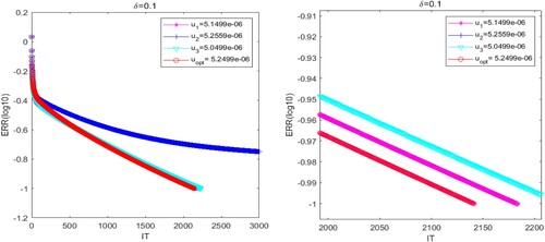
Table 1. Iterative number of the RGI algorithm with different μ for Example 5.1.

Display Table

Moreover, the RGI algorithm with $ω_{1} = ω_{2} = ω_{3} = ω_{4} = 0.5$ reduces to the GI algorithm. Similarly, we adopt the method of experiment debugging to find the optimal experimental parameter of the GI algorithm. Finally, the IT of the GI algorithm with $μ_{GI} = 4.5503 e - 06$ is the least.

In Figures –, we present that the convergence curves of the RGI and GI algorithms with different δ. In this experiment, we compare the convergence curves of two algorithms under the optimal experimental parameters. It follows from Figures – that the ERR decreases as the IT increases and gradually approaches 0, which indicates that the tested algorithms are effective and convergent. In addition, Figures – clearly show that the IT of the RGI and GI algorithms are decreasing as the increasing of δ. Besides, we can find that the convergence speed of the RGI algorithm is always faster than the GI one in the above four situations.

In order to more specifically verify the advantages of the RGI algorithm, we list detailed numerical results of the RGI and GI algorithms in Table , which includes IT, CPU and ERR. According to Table , the IT and CPU of the tested algorithms are gradually increase with the decreasing of the parameter δ. Moreover, it can be seen that the IT and CPU of the RGI method are always less than the GI one. Therefore, we can conclude that the convergence performance of the RGI algorithm proposed in this paper is better than the GI algorithm [Citation23].

Figure 2. The convergence curves of the tested methods with $δ = 0.1$ (left) and $δ = 0.01$ (right) for Example 5.1.

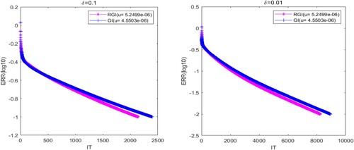
Figure 3. The convergence curves of the tested methods with $δ = 0.001$ (left) and $δ = 0.0001$ (right) for Example 5.1.

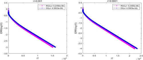
Table 2. Numerical results of the tested methods with different δ for Example 5.1.

Display Table

Example 5.2

We consider the generalized coupled complex conjugate and transpose Sylvester matrix equation (Equation1(1) $\begin{aligned} \sum_{j = 1}^{q} (A_{ij} Y_{j} B_{ij} + C_{ij} \bar{Y_{j}} D_{ij} \\ + E_{ij} Y_{j}^{T} F_{ij} + G_{ij} Y_{j}^{H} H_{ij}) = M_{i}, i \in I [1, p], \end{aligned}$ (1) ) in the special case of p = q = 2, and it has (82) ${\begin{cases} A_{11} Y_{1} B_{11} + C_{11} \bar{Y_{1}} D_{11} \\ + E_{12} Y_{2}^{T} F_{12} + G_{12} Y_{2}^{H} H_{12} = M_{1}, \\ A_{21} Y_{1} B_{21} + C_{21} \bar{Y_{1}} D_{21} \\ + E_{22} Y_{2}^{T} F_{22} + G_{22} Y_{2}^{H} H_{22} = M_{2}, \end{cases}$ (82) with the following parametric matrices $\begin{aligned} A_{11} & = [\begin{array}{ccc} 3 & - 5 & - 6 \\ - 1 + 7 i & - 5 + 3 i & 1 \\ - 2 + 7 i & - 9 + 6 i & 0 \end{array}], \\ B_{11} & = [\begin{array}{ccc} - 3 + 8 i & 2 - 9 i & - 3 \\ - 1 + 4 i & - 3 + 11 i & 10 \\ 1 + 8 i & 2 + 6 i & - 3 + 1 i \end{array}], \\ A_{21} & = [\begin{array}{ccc} 5 - 3 i & 1 & 14 - 3 i \\ 1 - 6 i & - 1 + 11 i & 1 + 14 i \\ 7 & 9 - 5 i & 1 + 3 i \end{array}], \\ B_{21} & = [\begin{array}{ccc} - 1 & 3 & 5 \\ 1 & - 3 & 1 \\ 1 & 2 & - 3 \end{array}], \end{aligned}$ $\begin{aligned} C_{11} & = [\begin{array}{ccc} 14 + 2 i & 3 + 5 i & 4 - 1 i \\ - 6 - 6 i & - 8 - 1 i & 5 + 1 i \\ 2 + 3 i & - 8 + 2 i & 1 - 9 i \end{array}], \\ D_{11} & = [\begin{array}{ccc} - 13 + 1 i & - 11 + 6 i & - 11 - 2 i \\ 2 + 7 i & - 10 + 4 i & - 10 + 1 i \\ - 2 + 5 i & 12 - 18 i & 1 - 9 i \end{array}], \\ C_{21} & = [\begin{array}{ccc} 8 - 2 i & - 8 - 2 i & - 5 i \\ 2 + 7 i & - 10 + 4 i & - 10 + 1 i \\ - 2 + 5 i & 12 - 18 i & 1 - 9 i \end{array}], \\ D_{21} & = [\begin{array}{ccc} - 12 + 1 i & - 10 + 6 i & - 20 \\ 2 + 7 i & - 10 + 4 i & - 10 + 1 i \\ - 2 + 5 i & 12 - 18 i & 1 - 9 i \end{array}], \end{aligned}$ $\begin{aligned} E_{12} & = [\begin{array}{ccc} 1 + 8 i & 6 - 2 i & - 8 + 17 i \\ 4 + 2 i & 10 + 9 i & 2 + 9 i \\ - 5 - 3 i & 4 + 10 i & 10 + 9 i \end{array}], \\ F_{12} & = [\begin{array}{ccc} 11 + 2 i & 2 - 8 i & 2 - 3 i \\ 7 + 7 i & 9 - 1 i & 1 + 5 i \\ 7 + 10 i & 5 + 8 i & 7 - 8 i \end{array}], \\ E_{22} & = [\begin{array}{ccc} 1 & - i & 1 \\ i & 1 & 1 \\ - 1 & 1 & 1 \end{array}], F_{22} = [\begin{array}{ccc} 1 & 2 & 2 \\ 1 & 0 & 0 \\ 0 & 1 & - 3 \end{array}], \\ G_{12} & = [\begin{array}{ccc} 1 & 1 & - 1 \\ 1 & 4 & 1 \\ - 2 & 0 & - 2 \end{array}], H_{12} = [\begin{array}{ccc} 1 & 2 & 2 \\ 1 & 0 & 0 \\ 0 & 1 & 1 \end{array}], \\ G_{22} & = [\begin{array}{ccc} 1 & 1 & - 1 \\ 1 & 4 & 1 \\ - 2 & 0 & - 2 \end{array}], H_{12} = [\begin{array}{ccc} 1 & 0 & - 1 \\ - 1 & - i & 1 \\ - 1 & 2 & 1 \end{array}], \end{aligned}$ $\begin{aligned} M_{1} & = [\begin{array}{cc} - 4792 + 2166 i & 2299 + 5490 i \\ 4679 + 3574 i & - 3507 - 629 i \\ - 2720 - 2137 i & - 4833 + 2642 i \end{array} \\ \begin{matrix} 3353 - 3607 i \\ 1933 - 1090 i \\ 2164 + 163 i \end{matrix}], \\ M_{2} & = [\begin{array}{cc} 562 + 1926 i & 356 + 452 i \\ - 1858 + 1250 i & 1113 + 610 i \\ - 511 + 863 i & 677 - 3228 i \end{array} \\ \begin{matrix} 1636 + 492 i \\ 2678 + 3267 i \\ 346 - 3251 i \end{matrix}] . \end{aligned}$ It has the exact solution $\begin{aligned} Y_{1} & = [\begin{array}{ccc} 2 + 2 i & 2 - 2 i & 1 \\ 1 & - 1 & 2 i \\ 2 - 2 i & 2 + 2 i & - 1 \end{array}], \\ Y_{2} & = [\begin{array}{ccc} 16 + 16 i & 20 - 28 i & 12 + 4 i \\ 29 - 4 i & - 7 + 5 i & - 4 + 17 i \\ 10 - 19 i & 9 + 11 i & - 1 - 2 i \end{array}] . \end{aligned}$

The initial iterative matrices are taken to be $Y_{i} (0) = 10^{- 6} \times I_{3}, i \in I [1, 2]$ . Then, we denote the relative iterative error by (83) $ERR = \frac{\sqrt{‖ Y_{1} - Y_{1} (k) ‖^{2} + ‖ Y_{2} - Y_{2} (k) ‖^{2}}}{\sqrt{‖ Y_{1} ‖^{2} + ‖ Y_{2} ‖^{2}}} .$ (83) In this example, all runs are stopped once ERR is less than ξ or k reaches the maximal iterative steps $k_{max} = 50,000$ . Here, ξ is a positive number.

For Example 5.2, we also compare the convergence performance of the RGI and GI algorithms. The optimal convergence parameters involved in two algorithms are determined by the following method. If relaxation factors are selected as $ω_{1} = 0.07, ω_{2} = 0.18$ , the optimal convergence factor of the RGI algorithm is adopted as $μ_{RGI} = 1.0821 e - 04$ by Theorem 4.1. Moreover, the RGI algorithm with $ω_{1} = ω_{2} = 0.5$ reduce to the GI algorithm. By some calculations, the best convergence parameter of the GI algorithm is $μ_{GI} = 4.5361 e - 05$ .

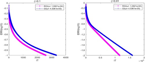
In Figures –, we plot the graphs of ERR(log10) versus the IT of the RGI and GI algorithms with different ξ. According to the convergence curves, we observe that the two algorithms are both convergent and efficient. It is obvious that the convergence rate of the RGI method ( $ω_{1} = 0.07, ω_{2} = 0.18$ ) is always faster than GI one ( $ω_{1} = ω_{2} = 0.5$ ) for the four cases of ξ. In addition, it follows from Figures – that the IT and CPU of the tested algorithms are increasing with the decreasing of ξ. In particular, the convergence advantage of the RGI algorithm is more obvious when ξ is smaller. The results illustrate that the RGI algorithm is superior to the GI algorithm if the relaxation parameters are chosen appropriately.

Figure 4. The convergence curves of the tested methods with $ξ = 0.1$ (left) and $ξ = 0.01$ (right) for Example 5.2.

In order to further verify the advantages of the proposed algorithm, we clearly report the numerical results of the RGI and GI methods for Example 5.2 in Table . From Table , it is easy to discover that the IT of the algorithms is increasing with the decreasing of relative error. Furthermore, the IT and CPU of the RGI method are less than those of the GI one. As a whole, the proposed algorithm has better convergence behaviours than the GI method. This means that the relaxation technique can effectively improve the convergence rate of the GI algorithm.

Figure 5. The convergence curves of the tested methods with $ξ = 0.001$ (left) and $ξ = 0.0001$ (right) for of Example 5.2.

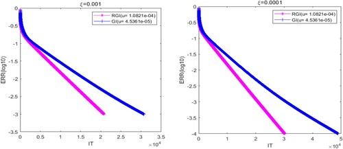
Table 3. Numerical results of the tested methods with different ξ for Example 5.2.

Display Table

6. Concluding remarks

In this paper, by adopting the relaxation technique into the GI algorithm, we establish the relaxed gradient-based iterative (RGI) algorithm to solve the generalized coupled complex conjugate and transpose Sylvester matrix equations. The main idea of the algorithm is introducing relaxation parameter to control the weights of iterative sequences. Applying straighten operation and real representation of complex matrices, we derive the necessary and sufficient condition for convergence of the RGI algorithm. Besides, the optimal convergence parameter and some related conclusions are given. To overcome high-dimensional computational problems, we propose sufficient condition for convergence with smaller computational complexity. Finally, numerical experiments verify that the RGI algorithm has more excellent convergence performance than the GI one.

Note that in our experiment, the relaxation factors $ω_{l}$ ( $l \in I [1, q]$ ) are obtained through experimental debugging. The selection criteria for the optimal relaxation factors are not provided. The future research direction is to further develop the theory of selecting the optimal relaxation factor. Besides, the value of the convergence parameter μ in the RGI algorithm is fixed. To optimize the convergence performance of the RGI algorithm, we will consider to introduce different step size factors into the RGI algorithm.

Supplemental material

Disclosure statement

No potential conflict of interest was reported by the author(s).

Additional information

Funding

This work is supported by the Guangxi Natural Science Foundations [No. 2021GXNSFBA196064, Guike AD21220129], the National Science Foundation of China [No. 11901123], the Guangxi Natural Science Foundations [2019GXNSFBA185014, Guike AD20159056], the Natural Science Foundation of Guangxi University for Nationalities [No. 2019KJQN001].

References

Hajarian M. Computing symmetric solutions of general Sylvester matrix equations via Lanczos version of biconjugate residual algorithm. Comput Math Appl. 2018;76:686–700. doi: 10.1016/j.camwa.2018.05.010
Web of Science ®Google Scholar
Hajarian M. Developing CGNE algorithm for the periodic discrete-time generalized coupled Sylvester matrix equations. Comput Appl Math. 2015;34:755–771. doi: 10.1007/s40314-014-0138-7
Google Scholar
Zhou Y-H, Zhang X, Ding F. Partially-coupled nonlinear parameter optimization algorithm for a class of multivariate hybrid models. Appl Math Comput. 2022;414:Article ID 126663.
Web of Science ®Google Scholar
Dehghan M, Hajarian M. The generalised Sylvester matrix equations over the generalized bisymmetric and skew-symmetric matrices. Int J Syst Sci. 2012;43:1580–1590. doi: 10.1080/00207721.2010.549584
Web of Science ®Google Scholar
Zhou B, Wei X-Z, Duan G-R. Stability and stabilization of discrete-time periodic linear systems with actuator saturation. Automatica. 2011;47:1813–1820. doi: 10.1016/j.automatica.2011.04.015
Web of Science ®Google Scholar
Zhou B, Duan G-R. Periodic Lyapunov equation based approaches to the stabilization of continuous-time periodic linear systems. IEEE Trans Automat Contr. 2011;57:2139–2146. doi: 10.1109/TAC.2011.2181796
Web of Science ®Google Scholar
Ding F, Wang F. Decomposition based least squares iterative identification algorithm for multivariate pseudo-linear ARMA systems using the data filtering. J Franklin Inst. 2017;354:1321–1339. doi: 10.1016/j.jfranklin.2016.11.030
Web of Science ®Google Scholar
Shen H-L, Peng C, Zhang T. Gradient based iterative solutions for Sylvester conjugate matrix equations. J Math Res Appl. 2017;03:103–118.
Google Scholar
Li X, Ding J, Ding F. Gradient based iterative solutions for general linear matrix equations. Comput Math Appl. 2009;58:1441–1448. doi: 10.1016/j.camwa.2009.06.047
Web of Science ®Google Scholar
Li X, Liu Y-J, Yang H-Z. Gradient based and least squares based iterative algorithms for matrix equations AXB+CXTD=F. Appl Math Comput. 2010;217:2191–2199.
Web of Science ®Google Scholar
Bai Z-Z, Guo X-X, Yin J-F. On two iteration methods for the quadratic matrix equations. Int J Numer Anal Model. 2005;2:114–122.
Web of Science ®Google Scholar
Chen Z-B, Chen X-S. Modification on the convergence results of the Sylvester matrix equation AX + XB = C. J Franklin Inst. 2022;359:3126–3147. doi: 10.1016/j.jfranklin.2022.02.021
Web of Science ®Google Scholar
Xu L, Ding F, Zhu Q-M. Separable synchronous multi-innovation gradient-based iterative signal modeling from on-line measurements. IEEE Trans Instrum Meas. 2022;71:1–13.
Web of Science ®Google Scholar
Ding F. Least squares parameter estimation and multi-innovation least squares methods for linear fitting problems from noisy data. J Comput Appl Math. 2023;426:Article ID 115107. doi: 10.1016/j.cam.2023.115107
Web of Science ®Google Scholar
Ding J, Liu Y-J, Ding F. Iterative solutions to matrix equations of the form AiXBi=Fi. Comput Math Appl. 2010;59:3500–3507. doi: 10.1016/j.camwa.2010.03.041
Web of Science ®Google Scholar
Ding F, Ding J. Iterative solutions of the generalized Sylvester matrix equations by using the hierarchical identification principle. Appl Math Comput. 2008;197:41–50.
Web of Science ®Google Scholar
Ding F, Chen T-W. Gradient based iterative algorithms for solving a class of matrix equations. IEEE Trans Automat Contr. 2005;50:1216–1221. doi: 10.1109/TAC.2005.852558
Web of Science ®Google Scholar
Ding F, Chen T-W. On iterative solutions of general coupled matrix equations. SIAM J Control Optim. 2006;44:2269–2284. doi: 10.1137/S0363012904441350
Web of Science ®Google Scholar
Ding F, Chen T-W. Iterative least-squares solutions of coupled Sylvester matrix equations. Syst Control Lett. 2005;54:95–107. doi: 10.1016/j.sysconle.2004.06.008
Web of Science ®Google Scholar
Wu A-G, Zeng X-L, Duan G-R, et al. Iterative solutions to the extended Sylvester-conjugate matrix equations. Appl Math Comput. 2010;217:130–142.
Web of Science ®Google Scholar
Wu A-G, Feng G, Duan G-R, et al. Iterative solutions to coupled Sylvester-conjugate matrix equations. Comput Math Appl. 2010;60:54–66. doi: 10.1016/j.camwa.2010.04.029
Web of Science ®Google Scholar
Song C-Q, Chen G-L, Zhao L-L. Iterative solutions to coupled Sylvester-transpose matrix equations. Appl Math Model. 2011;35:4675–4683. doi: 10.1016/j.apm.2011.03.038
Web of Science ®Google Scholar
Beik FPA, Mahmoud MM. Gradient-based iterative algorithm for solving the generalized coupled Sylvester-transpose and conjugate matrix equations over reflexive (anti-reflexive) matrices. Trans Inst Meas Control. 2014;36:99–110. doi: 10.1177/0142331213482485
Web of Science ®Google Scholar
Lv L-L, Chen J-B, Zhang L, et al. Gradient-based neural networks for solving periodic Sylvester matrix equations. J Franklin Inst. 2022;359:10849–10866. doi: 10.1016/j.jfranklin.2022.05.023
Web of Science ®Google Scholar
Li S-H, Ma C-F. Factor gradient iterative algorithm for solving a class of discrete periodic Sylvester matrix equations. J Franklin Inst. 2022;359:9952–9970. doi: 10.1016/j.jfranklin.2022.09.041
Web of Science ®Google Scholar
Fan W, Gu C-Q, Tian Z-L. Jacobi-gradient iterative algorithms for Sylvester matrix equations. In: Linear algebra society topics. Shanghai, China: Shanghai University; 2007. p. 16–20.
Google Scholar
Niu Q, Wang X, Lu L-Z. A relaxed gradient based algorithm for solving Sylvester equations. Asian J Control. 2011;13:461–464. doi: 10.1002/asjc.v13.3
Web of Science ®Google Scholar
Huang B-H, Ma C-F. The relaxed gradient-based iterative algorithms for a class of generalized coupled Sylvester-conjugate matrix equations. J Franklin Inst. 2018;355:3168–3195. doi: 10.1016/j.jfranklin.2018.02.014
Web of Science ®Google Scholar
Huang B-H, Ma C-F. On the relaxed gradient-based iterative methods for the generalized coupled Sylvester-transpose matrix equations. J Franklin Inst. 2022;359:10688–10725. doi: 10.1016/j.jfranklin.2022.07.051
Web of Science ®Google Scholar
Wang W-L, Song C-Q, Ji S-P. Iterative solution to a class of complex matrix equations and its application in time-varying linear system. J Appl Math Comput. 2021;67:317–341. doi: 10.1007/s12190-020-01486-6
Web of Science ®Google Scholar
Ding F. Hierarchical multi-innovation stochastic gradient algorithm for Hammerstein nonlinear system modeling. Appl Math Model. 2013;37:1694–1704. doi: 10.1016/j.apm.2012.04.039
Web of Science ®Google Scholar
Wu A-G, Zhang Y, Qian Y-Y. Complex conjugate matrix equations. Beijing: Science Press; 2017.
Google Scholar
Ding F, Chen T-W. Hierarchical gradient-based identification of multivariable discrete-time systems. Automatica. 2005;41:315–325. doi: 10.1016/j.automatica.2004.10.010
Web of Science ®Google Scholar
Zhang H-M. A finite iterative algorithm for solving the complex generalized coupled Sylvester matrix equations by using the linear operators. J Franklin Inst. 2017;354:1856–1874. doi: 10.1016/j.jfranklin.2016.12.011
Web of Science ®Google Scholar

The relaxed gradient based iterative algorithm for solving the generalized coupled complex conjugate and transpose Sylvester matrix equations

Abstract

1. Introduction

2. Preliminaries

[Citation28]

[Citation32]

[Citation28]

[Citation33]

[Citation29]

[Citation28]

[Citation28]

[Citation29]

3. The relaxed gradient-based iterative algorithm

4. Convergence analysis of the RGI algorithm

5. Numerical experimental results

[Citation34]

Table 1. Iterative number of the RGI algorithm with different μ for Example 5.1.

Table 2. Numerical results of the tested methods with different δ for Example 5.1.

Table 3. Numerical results of the tested methods with different ξ for Example 5.2.

6. Concluding remarks

example1.pdf

u111.eps

u1u2u3.pdf

example2.pdf

x3.eps

x2.eps

x1.eps

x2.pdf

q2.eps

x4.pdf

q2.pdf

q3.eps

q4.pdf

u111.pdf

x4.eps

q1.pdf

example01.pdf

q3.pdf

u222.pdf

x3.pdf

x1.pdf

q1.eps

q4.eps

u222.eps

Disclosure statement

Additional information

Funding

References

Related research

To cite this article:

Download citation

Your download is now in progress and you may close this window

Login or register to access this feature

Information for

Open access

Opportunities

Help and information

Keep up to date