Fine-scale selection of nesting habitat in Little Crake Porzana parva and Water Rail Rallus aquaticus in small ponds

Abstract

Capsule The most important factor determining fine-scale selection of nesting habitat in Little Crake and Water Rail is water depth.

Aims To evaluate factors affecting nest-site selection and relative inter-specific differences in two poorly studied Rallidae species, the Little Crake and Water Rail.

Methods Habitat variables describing water depth, water cover, as well as vegetation type and structure were measured within 3-m radius plots around birds' nests and random points, located in small ponds scattered within a largely cultivated landscape in north-eastern Poland. Descriptive statistics and multi-adaptive regression splines were used to describe nesting habitat and to model nest-site selection in the study species.

Results Little Crake nested in sites with deeper water and lower percentage of vegetation cover than Water Rail. Both species chose nest sites according to water depth (probability of Little Crake nests occurrence was the highest around 40 cm and of Water Rail below 12 cm) and vegetation stage in which nests were build (old vegetation was preferred). Little Crake nests were also associated with vegetation height lower than 1.5 m and high percentage cover of old vegetation within a 3-m radius around nests, whereas Water Rail preferred Carex spp. and Juncus effusus for nesting.

Conclusion For both species, water depth was the main driver of nest-site selection, followed by vegetation traits. Water depth was also the variable most important in discriminating between the nesting sites of the two species. The different patterns of habitat selection showed by the two species are likely to be due to different morphology and nest characteristics, and are probably driven by the need to maximize both nest and adult safety.

Habitat selection is the process determining the choice of a particular habitat amongst others available (Patridge 1978), and is often considered as a hierarchical process (Hutto 1985, Saab 1999, Harvey & Weatherhead 2006). Different environmental features (food availability, vegetation structure and social factors) may be responsible for habitat selection at different levels (Burger 1985, Anderson et al. 2005, Mayor et al. 2009). In birds, during the breeding season, the final step in this hierarchical process is the selection of the nest site, after more general choices at the landscape and territory level (Jones & Robertson 2001, Martinez et al. 2003, Bailey & Thompson 2007). In many species, the most important factor for nest-site selection seems to be the vegetation structure in close proximity to the nest (Burger 1985, Orians & Wittenberger 1991). Because for most birds, the main cause of nest failure is predation (Ricklefs 1969), it has been posited that birds choose their nest sites according to the vegetation structure, which has a direct influence on the probability of nest detection by predators, and thus on brood survival (Møller 1989, Martin 1993, Sieving & Willson 1998, Liebezeit & George 2002, Baxter et al. 2009).

This study focuses on the nest-site selection process of two marsh-nesting bird species belonging to the Rallidae family, the Little Crake Porzana parva and the Water Rail Rallus aquaticus. Members of this family are specially adapted to live and move smoothly in dense vegetation with their laterally compressed body and relatively long legs and toes (Del Hoyo et al. 1996, Taylor & Van Perlo 1998). This high specialization may influence the preferences and selection of particular vegetation types and structure in the breeding site in contrast to other waterbirds. Both Little Crake and Water Rail occupy a wide range of freshwater, usually eutrophic wetlands (natural and semi-natural), with fairly tall and dense aquatic vegetation (Cramp 1980, Taylor & Van Perlo 1998). A few recent studies have investigated landscape and spatial determinants of Water Rail occurrence or abundance (Jenkins & Ormerod 2002, Brambilla & Rubolini 2004, Brambilla et al. 2012), but small-scale nest-site preferences of both species are poorly known (Schiermann 1929, Kux 1959, De Kroon 2000, De Kroon & Mommers 2002, De Kroon 2004), although water depth at nest sites has been reported to vary between the two species, with Water Rail nesting in shallower places than Little Crake (Bauer 1960). Nevertheless, virtually no study has quantitatively analysed which habitat features are most likely to drive nest-site selection in these two secretive species.

The aim of the present study was thus (1) to describe the habitat factors within a 3-m radius plot around birds' nests (related to water depth and cover, vegetation structure, type and cover) affecting nest-site selection and (2) to investigate whether the fine-scale nest-site preferences of Little Crake and Water Rail overlap or differ.

METHODS

Study area

The study was conducted in north-eastern Poland (the Mazurian Lake District), within a typical young post-glacial landscape, characterized by a large number of lakes and by many small inland water bodies (ponds). Until the 1990s, intensive agricultural practices were carried out in this area, which resulted in the draining of many of these wetlands. After the State Agricultural Farms collapsed in 1993, land-use practices changed and many fields were abandoned. Due to the lack of conservation of drainage channels, many small midfield water bodies started to recover in natural depressions. These changes were reinforced by the implementation of water retention and by the increasing abundance of Eurasian Beavers Castor fiber in this region in last two decades (Czech 2010), which has resulted in an increase in flooded sites and ponds.

Data were collected at 20 unnamed water bodies distributed at 53°48′–53°53′ N and 21°34′–21°44′ E. The area of these water bodies varied from 0.1 to 10.6 ha (mean 2.58 ha), the average depth was usually less than 2 m and water acidity pH ranged from 6.3 to 8.2 (mean 7.11). Most of the ponds were located in depressions filled by organic sediments, mainly peat. The vegetation of the littoral zone was typical for early stages of development. Most of the ponds were strongly dominated by typical hydrophytes such as Typha spp., Common Reed Phragmites australis and Carex spp., with some clumps of Grey Willow Salix cinerea. Water bodies were surrounded by agricultural (arable fields, meadows and pastures) or post-agricultural (fallows) lands.

Data collection

Data were collected from mid-April to the end of July in 2011–2013 by the same observer (J.J.). During these three breeding seasons, nests of Little Crake and Water Rail were searched for and habitat variables were measured around the nests and at the random points in the study area.

The high vocal activity of both species during the breeding season is helpful in estimating rail density and in finding nests (Taylor & Van Perlo 1998). Along the shore line of each water body, birds were stimulated every 50 m (Dombrowski et al. 1993) with a playback of their voices in the periods of their highest vocal activity, usually before sunrise and before sunset (Polak 2005, Brambilla & Jenkins 2009). To stimulate birds, we used 30-second long sequences of the announcement call of male Water Rails and of the advertising call of male Little Crakes (Cramp 1980). If birds responded to the vocal stimulation the site was marked on a 1:10000 map. If there was no response within 2 minutes, the stimulation was repeated. Monitoring was conducted every 10–14 days in each site (from mid-April to the end of June) and after confirming that birds responded from the same place during two consecutive controls, the vegetation around the marked places was systematically and carefully investigated. The position of each nest was marked using a handheld GPS receiver (Topcon GRS-1; accuracy less than 0.5 m). Also the stage of the nests was assessed at the time of finding (egg laying, incubating or nestling period), and the size of the clutch was also checked seven days later.

At each nest site and in a corresponding random point, 16 different habitat variables were recorded. The ‘Random points’ tool in QGIS 1.8.0 software was used to choose random points and a handheld GPS receiver to find them in the field. The random points were chosen separately for Little Crake and Water Rail in the littoral vegetation at the same water bodies as the birds' nests (for each pond, the number of random points equalled the number of nests for each species). Habitat variables were measured in a circular plot, defined as a 3-m radius around the nest or the random point (nest-site plots and random plots, respectively). The minimum distance between a nest and random point or among neighbouring random points was 6 m, so as to avoid non-independent variable recording due to plot overlap.

At nest-site and random plots the following habitat variables were measured: water depth at the centre of the plot (estimated with 1 cm precision), mean water depth (average value from ten randomly selected points within the plot), standard deviation for water depth, height of emergent vegetation at the centre of the plot (estimated from the water surface with 5 cm precision), mean vegetation height from ten randomly selected points within the plot and standard deviation for vegetation height. Emergent vegetation around nests and random points was identified to particular species, and the stage of vegetation growth was assigned to one of three categories: new (fresh vegetation), old (1 or more year-old vegetation) or mixed (old with new vegetation). The main plant species used as nest material was recorded in all nests. In each plot, the proportional area covered by new and old vegetation, and by open water was recorded. Percentage cover values were estimated with 5% precision. Old and new vegetation cover was estimated separately, because both covers usually overlap in clumped littoral vegetation (new vegetation growing over the old from the same clump). The proportional cover of the following vegetation categories was also determined (with 5% precision) at the nesting-site plots and in random plots: Typha spp. (Bulrush Typha latifolia and Lesser Bulrush Typha angustifolia), Common Reed, Carex spp. (mainly Lesser Pond-sedge Carex acutiformis and Greater Pond-sedge Carex riparia), Soft-rush Juncus effusus, Water-plantain Alisma plantago-aquatica, Reed Sweet-grass Glyceria maxima, Reed Canary-grass Phalaris arundinacea, Sweet-flag Acorus calamus, Wood Club-rush Scirpus sylvaticus, Amphibious Bistort Persicaria amphibia, Yellow Iris Iris pseudacorus, Water Horsetail Equisetum fluviatile, dicotyledon herbs (mainly Skullcap Scutellaria galericulata, Bittersweet Solanum dulcamara and Gypsywort Lycopus europaeus) and Grey Willow. Using these categories, the dominant vegetation was assessed within each plot and habitat heterogeneity was estimated according to Shannon diversity index (H = −Σp_iln p_i, where p_i is the proportion of the ith vegetation category within the nest or the random plot; Magurran 2004). Finally, the distances from the nest sites or the random points to the nearest shore, open water and Grey Willow shrub were measured (with 1 m precision), using QGIS 1.8.0 software and satellite photographs.

Statistical analyses

Multi-adaptive regression splines (MARS) were used to model habitat association in the study species, relating their occurrence to the set of environmental variables listed above. MARS is a recent machine-learning technique (Friedman 1991, Hastie et al. 2009), and thanks to its flexibility and ability to model non-linear relationships (Elith & Leathwick 2007), MARS is now increasingly used in ecology (Leathwick et al. 2005, Mac Nally et al. 2008, Heinanen & von Numers 2009, Brambilla & Gobbi 2014). This regression method fits non-linear functions by fitting linear segments (or piecewise linear basis functions) to the data, breaking predictors at knots, allowing the slope of segments to vary between knots and connecting adjacent segments at knots, thus keeping the full fitted function without gaps or steps. Model fitting is achieved by a forward procedure that identifies many potential predictors and knots, on the basis of a specified increase in model performance (the ‘threshold’), followed by backward pruning that reduces the number of predictors and knots on the basis of a penalty value.

Prior to multivariate analyses, variable correlations were checked. Although variable autocorrelation has been reported to be less problematic for machine-learning than for statistical methods, it may still affect models (Merow et al. 2013) and in particular the interpretation of the effects of habitat factors on species' response. Therefore, for pairs of variables which were highly intercorrelated (r > 0.7, P < 0.05), only one of the two was alternatively entered in the analyses, and thus different sets of models were tested, excluding different variables each time (see Supplementary online material). The earth package version 3.2-1 (http://cran.r-project.org/web/packages/earth/index.html) in R 3.0.1 (R Development Core Team 2013) was used. The earth package allows MARS analyses for different types of distribution, including binomial distributions (Milborrow 2011a), which was used for the model with nest and random plots of Little Crake and Water Rail, respectively, as the dependent variable. The following settings, commonly adopted as default values, were used for model selection: threshold = 0.001, penalty = 2 and degree of interactions = 1 (no interaction allowed among variables). The model was subjected to cross-validation, which was used to estimate model performance over different subsets of the data. The number of folders for cross-validation was five for Water Rail, and two for Little Crake, given that for the latter increasing the number of folders resulted in too high a standard deviation. The discriminatory ability of the models was evaluated by means of the area of the curve of the receiver operating characteristic plot, calculated considering the cross-validation output. Variable importance was evaluated on the basis of the evimp command (Milborrow 2011a, Brambilla et al. 2013). The evimp command estimates variable importance in a MARS model according to three criteria: (1) the number of model subsets generated by the pruning pass, which include a given variable: variables included in more subsets are considered more important; (2) the decrease in the residual sum of squares (RSS) for each subset relative to the previous subset: for each variable evimp sums these decrease over all subsets that include the variable and rescales the summed decreases to a percentage scale (largest one equal to 100); (3) the generalized cross-validation (GCV) of the model, calculated using the penalty argument, which considers the increase or decrease in the GCV associated with a variable being added to the model; the evimp command uses GCV criterion exactly like the RSS criterion (Milborrow 2011a). The plotmo package version 1.3-1 (http://cran.r-project.org/web/packages/plotmo/index.html) was used to plot the fitted functions (Milborrow 2011b). After repeating the same procedure for all subsets of variables, the models which showed both the inclusion of relevant variables and good cross-validation statistics were selected, indicating model robustness and consistency across data (Supplementary online material). When two models received the same statistical support, the simplest one was selected. The two most correlated variables were water depth and mean water depth. Models including the latter were preferred, because it seemed that depth in the close surroundings of the nest could be more important in determining nest accessibility (both to breeding species and predators), rather than the depth at a very specific point. In any case, all models tested are reported in the Supplementary online material.

To assess what factors differ in habitat selection between the two species, we built a further model using all data, with nest presence/absence as dependent variables, and as predictors the most relevant (according to species-specific models) and weakly correlated habitat variables (mean water depth, vegetation height, vegetation type, vegetation stage, distance from bank, distance from open water, distance from bushes and percentage of old vegetation) and species as a factor. We then tested the effect of the interaction of habitat predictors by species, to evaluate variables subjected to different selection by the two species. We adopted the same MARS procedure described above also for this analysis.

RESULTS

Nest-site features

During the three breeding seasons, 70 nests of Little Crake and 37 nests of Water Rail were found. The earliest nests were found on 30 April for Water Rail and on 6 May for Little Crake. The latest nests were found on 11 July for Water Rail and on 25 July for Little Crake. Nineteen nests of Little Crake and 30 nests of Water Rail were recorded during the egg-laying period. Five nests of each species were found as abandoned after predation. The rest of the nests were recorded during the incubation period. Distance between neighbouring nest of Little Crake averaged 75.9 m (sd ± 43.3 m, n = 58), between Water Rail nests averaged 122.4 m (sd ± 36.0 m, n = 16) and between two nearest nests of both species was an average of 80.3 m (sd ± 49.8 m, n = 31). Little Crake nested on 14 water bodies with mean density 1.07 pairs/ha and Water Rail on 16 water bodies with mean density 0.75 pair/ha. Water Rail and Little Crake co-occurred on half of the water bodies studied with overall breeding density 1.64 pairs/ha.

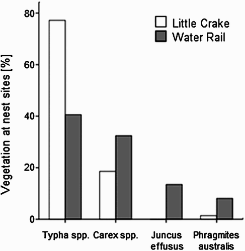
Both species nested mainly in Typha spp. and Carex spp. (Fig. 1). Single nests of Little Crake were also found in Common Reed, Water-plantain and in Reed Sweet-grass (each 1.4%). Water Rail nested occasionally in Soft-rush (13.5%), Common Reed (8.1%), Reed Canary-grass (2.7%) and in Sweet-flag (2.7%). The vegetation category around the nests was the same as the dominant vegetation within the 3-m radius plots in 92.9% of plots for Little Crake and in 75.7% of plots for Water Rail. Little Crake and Water Rail built nests mostly in mixed (respectively, 62.8% and 48.6%) and old vegetation (respectively, 32.9% and 46.0%), and only sporadically in new vegetation (respectively, 4.3% and 5.4%). The commonest nest materials used by both species were old leaves of Typha spp., found in 87.1% of Little Crake nests and in 75.7% of Water Rail nests (the rest of the nests were built with Carex spp. and two nests of Water Rail were built with Common Reed). Comparing nest material with dominant vegetation in nest plots, the ratio between Typha spp. and other vegetation categories did not significantly differ for Little Crake (χ² ₁ = 0.2, P = 0.63) and for Water Rail (χ² ₁ = 3.8, P = 0.051).

Figure 1. Frequency of the most common vegetation types at nesting sites of Little Crake and Water Rail.

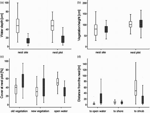
Water depth (mean ± se) at Little Crake nest sites was 48.5 ± 2.25 cm (range 10–100 cm) and 14.4 ± 1.31 cm (range 2–30 cm) at Water Rail nest sites, and the former preferred also deeper mean water depth (Fig. 2a). Emergent vegetation height at Little Crake nest sites was 81.4 ± 3.67 cm and 81.7 ± 4.42 cm at Water Rail nest sites (the average height of vegetation within nest plots were slightly higher; see Fig 2b). The nest plots of Little Crake were characterized also by 36.6 ± 1.86% of old vegetation cover, 32.4 ± 1.97% of new vegetation cover and by 51.1 ± 1.43% of open water cover. Respective values for Water Rail nest plots were 54.3 ± 3.33%, 41.6 ± 4.56% and 28.9 ± 2.39% (Fig 2c). Habitat heterogeneity was higher within Water Rail nest plots (0.54 ± 0.05) than within Little Crake nest plots (0.19 ± 0.04). Finally, the nests of Little Crake were situated closer to the open water than Water Rail nests (respectively, 4.0 ± 0.52 m and 23.7 ± 3.99 m), further from willow shrubs (respectively, 56.8 ± 4.59 m and 23.5 ± 5.02 m) and at a similar distance to dry areas (respectively, 10.0 ± 0.90 m and 9.6 ± 1.62 m; see Fig. 2d). Despite these recorded differences, the range of values for all environmental variables recorded at Little Crake and Water Rail nest sites overlapped. The summary of all measurements taken in nest sites of Little Crake and Water Rail, as well as in random points are shown in the Supplementary online material.

Figure 2. Comparison of habitat variables at nesting sites and nesting plots (area within 3-m radius around nest) of Little Crake (white box plots) and Water Rail (grey box plots): (a) water depth at nest site and mean water depth at nest plot; (b) vegetation height at nest site and mean vegetation height at nest plot; (c) percentage cover of old and new vegetation, and open water cover at nest plot; (d) distances from the nest to the nearest shore, open water and Grey Willow shrub. The band inside the box represents the median and whisker plots represent range of values without outliers.

Habitat selection models

The selected MARS model for Little Crake included four variables: mean water depth, percentage cover of old vegetation within a 3-m radius plot, vegetation height and vegetation stage at the centre of the plot (Table 1). Nest occurrence probability peaked at sites with mean water depth equal to 42 cm, vegetation height lower than 146 cm, percentage cover of old vegetation higher than 40% and vegetation stage old or new (not mixed, see Fig. 3). The evimp command for the evaluation of the variable importance confirmed model strength, indicating that the included variables were the ones considered as more important (Table 1), whereas possible importance is additionally suggested for distance to bushes (number of subset 1, RSS 13.2 and GCV 30.4), that was not included in the chosen model. This model was very close (the same variables were selected and with the same effect) to a model obtained using water depth at nesting sites/random points instead of mean water depth (see Supplementary online material), further suggesting the model's validity.

Figure 3. Graphical summary of the MARS model for nesting-site selection in Little Crake. Species–habitat relationships show the probability of nest occurrence in relation to mean water depth (cm), vegetation height (cm), vegetation stage (old, new, mixed) and percentage cover of old vegetation (% cover in the 3-m radius around the nest). Sunflower plots (upper row: nests; lower row: random points) are also shown in each graph.

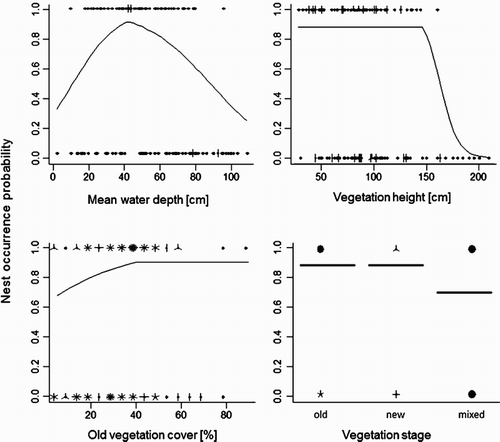
Table 1. Summary of selected MARS models (see text and Supplementary online material) for the two studied species.

Variable	Coefficient	No. of subsets	RSS	GCV
Little Crake
(R^2 = 0.28, cv R^2 ± sd = 0.17 ± 0.01, AUC ± sd = 0.74 ± 0.00)
Intercept	2.66
Mean water depth (below 42 cm)	0.05	100.0	5	5
Mean water depth (above 42 cm)	−0.08
Vegetation height (above146 cm)	−0.12	1	11.7	29.8
Old vegetation cover (below 40%)	0.04	1	11.7	29.8
Vegetation stage mixed	−1.18	3	45.1	60.0
Water Rail
(R^2 = 0.52, cv R^2 ± sd = 0.36 ± 0.09, AUC ± sd = 0.86 ± 0.07)
Intercept	2.54
Mean water depth (above 12 cm)	−0.12	4	100.0	100.0
Vegetation type Carex spp.	2.67	2	37.9	46.1
Vegetation type J. effusus	17.68	1	25.5	31.4
Vegetation stage mixed	−2.73	3	48.7	58.9

For complex hinge functions, the effect for the specified range of values is reported; see Figs 3 & 4 for a detailed description of the species–habitat variables. Abbreviation: no. of subset, number of model subsets generated by the pruning pass, which include a given variable; RSS, decrease in the residual sum of squares; GCV, generalized cross-validation of the model; R², model's R²; cv R² ± sd: model's R² calculated over the cross-replicated models and the relative standard deviation; AUC ± sd: the area under the curve (and its standard deviation) calculated over the cross-replicated models. See text for explanation.

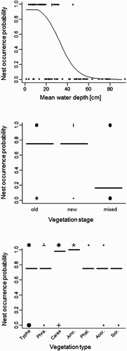
The selected MARS model for Water Rail included mean water depth, vegetation stage and vegetation category at the centre of the plot (Table 1). Nest occurrence probability was highest at sites with mean water depth lower than 12 cm, vegetation stage old or new (not mixed) and in sites with Carex spp. or J. effusus (Fig. 4). The evimp command for the evaluation of variable importance confirmed model strength, indicating that the included variables were the ones regarded as more important (Table 1).

Figure 4. Graphical summary of the MARS model for nest-site selection in Water Rail. Species–habitat relationships show the probability of nest occurrence in relation to mean water depth (cm), vegetation stage (old, new and mixed) and vegetation category (in the order: Typha spp., P. australis, Carex spp., J. effusus, P. arundinacea, A. calamus and S. sylvaticus). Sunflower plots (upper row: nests; lower row: random points) are also shown in each graph.

The MARS model considering the effects of species-habitat interactions revealed that the variable most important in discriminating between the two nest-site selection processes was mean water depth (details not shown), in agreement with the variable's importance separately for both Little Crake and Water Rail, and with the different effect on nest occurrence probability for the two species shown by the species-specific models.

DISCUSSION

Our work represents one of the first quantitative descriptions of nesting habitat in these poorly investigated Rallid species (Stermin 2012). Despite the overlap in the range of values recorded for habitat features at nest sites and nesting plots of the two species, the average nesting habitat of the two species was quite different. The most pronounced differences were found in water levels, consistent with earlier studies reporting water levels at Little Crake nest sites ranging from 30 to 60 cm (Kux 1959, Dittberner & Dittberner 1990), and at Water Rail nest sites ranging from 3 to 16 cm (De Kroon 1999). According to our results, the water depth at Little Crake nest sites was, on average, 34 cm higher than that found at Water Rail nest sites, although 17% of Little Crake nests were located in places potentially acceptable for Water Rail too (water depth lower than 30 cm). This result suggests that nest sites of both species may potentially co-occur in places where the water level is between 10 and 30 cm. In summary, water level was the most important factor driving nest-site selection and was clearly associated with a different response pattern from the two species (see Results and Figs 3 & 4).

For marsh-nesting birds, water depth is related to the pressure of terrestrial predators and deeper zones ensure greater nesting success (Jobin & Picman 1997, Hoover 2006). On the other hand, denser vegetation cover provides security against bird predators (Dwernychuk & Boag 1972), as well as terrestrial predators (Schranck 1972). For the Water Rail and Little Crake predator pressure is still poorly known, but it seems that in the Mazurian Lakeland the main nest predators are the Marsh Harrier Circus aeruginos and species belonging to the Mustelidae family (J. Jedlikowski, unpubl. data), suggesting that the safest places should be in deeper water, surrounded by dense vegetation cover. As the water depth in ponds was negatively correlated with the density of vegetation cover (r > 0.7, P < 0.001 for both species), birds had to optimize their choice between these two variables during nest-site selection.

One of the main differences in breeding biology between both species, which may potentially be related to the process of nest-site selection, is nest size and egg pigmentation. Water Rail nests are bigger than Little Crake nests (the average outside diameter is 20 cm (De Kroon 2004) and 13 cm (J. Jedlikowski, unpubl. data), respectively), and contain off-white eggs different from the more cryptic and smaller brown-buff eggs of Little Crake (Taylor & Van Perlo 1998). This suggests that a Water Rail clutch is probably more visible (especially by aerial predators) and thus birds have to choose places with denser vegetation cover.

Furthermore, both species are adapted to walking through littoral vegetation and they use floating plant material (leaves and stems) as a walking path. They prefer running through dense vegetation than swimming or flying when they are threatened (Taylor 1980, Taylor & Van Perlo 1998, own observations). Because Water Rail are at least 15% larger and on average twice as heavy as the biggest Little Crake (Cramp 1980), the buoyancy of this species is less. In deeper zones of littoral vegetation, cover and floating plant material are less dense (Grace 1989), therefore Water Rail would have to swim and fly more often there, and so may be more vulnerable to predation. The Little Crake is lighter and moves more easily even in places with scarce floating plant material.

Considering these two differences: in morphology and in clutch characteristics, it can be supposed that each species then selects the safest nesting sites in relation to their respective characteristics. Water Rails nested in shallow plots with vegetation cover 16% denser than random plots and 22% denser than Little Crake plots, which may reduce visibility of the nest and provide better security also for adult birds. Little Crakes can nest in deeper littoral waters, which provide better protection from terrestrial mammalian predators, likely because of its lighter weight which enables the use of sparser floating stems and leaves of the deeper areas.

The different predominance of vegetation types around the nest sites of the two species may also reflect different anti-predator strategies in Water Rail and Little Crake. The compact clumps of old Typha spp., which were 17.2% more frequent at Little Crake nest sites than at comparative random points, may well hide the nest, and enable safe movements of adult birds. In contrast, nests situated in Common Reed patches are characterized probably by a higher level of vertical visibility, and thus may be more easily found by terrestrial mammals. Similar results for Little Crake were obtained by Glutz von Blotzheim et al. (1973), who found 58% (15) nests in Typha spp. and only 19% (5) nests in Common Reed. The preferences for particular vegetation at nest sites are probably driving the association with vegetation height too. A decreasing probability of nest occurrence in places with vegetation height above 150 cm corresponds to the maximum height of Typha spp. stems – 160 cm, in contrast to Common Reed steams, which had an upper limit of 210 cm.

Similarly, Water Rails nested mainly in Typha spp. and Carex spp. Slightly different results were obtained by De Kroon (1999), who found most nests in Carex spp. (73%) and the rest in Common Reed (27%). However, in our study the highest probability of Water Rail nest occurrence was in Soft-rush and Carex spp. (Fig. 4). A large clump of Juncus spp. and Carex spp. may provide excellent protection of nests from all sides, and reduce its vulnerability. Accordingly, De Kroon (2004) found that nests and eggs of Water Rail placed in Sea Rush Juncus maritimus were less visible than those situated in Common Reed mixed with Carex spp.

Both species show a preference for nesting in old vegetation. At the beginning of the breeding season old vegetation is the only type where birds may find sufficient cover to build nests, and even later in the season the compacted clumps of dead steams create an excellent ‘roof’, which may protect against predators and severe weather conditions (hot sun and rain). The previous year's stems and leaves seem to be also crucial as nest material for both species. All the nests found in this study were built using old plant material. Probably such material is easier to collect by the birds than fresh stems and leaves.

Previous studies have reported that Water Rail nests are usually situated in close proximity to bushes (Huygens 1954, De Kroon 2000). Such places are used as roosting sites and provide safe havens for chicks and adult birds (pers. obs.). Our study shows that nests of Water Rail were closer to willow shrubs than random points, nevertheless this factor was not included in the habitat-preference models. In the case of Little Crake, nests were located further from willow shrubs than random points, but values varied a lot, and the MARS model did not provide a definitive confirmation for such a pattern and thus a real avoidance of shrubs is questionable.

Our results may have some implications for the conservation and management of habitats with breeding Little Crakes and Water Rails. Potentially, the most important factors to be considered for their conservation through habitat management are avoiding the complete removal of old vegetation, such as dead stems or leaves, keeping a fine-scaled mosaic of open water and vegetation cover and managing water level consistent with the two species' different requirements.

Supplemental Data

comparing vegetation and habitat variables of Little Crake and Water Rail nests with random sites, and details of the MARS models of nest-site selection can be accessed at http://dx.doi.org/10.1080/00063657.2014.904271

ACKNOWLEDGEMENTS

We are grateful to M. Brzeziński for valuable comments on the manuscript. The study was carried out at the Biological and Chemical Research Centre, University of Warsaw, established within the project co-financed by European Union from the European Regional Development Fund under the Operational Programme Innovative Economy, 2007–2013.

Funding

This work was supported by the National Science Centre of Poland [grant number N N305 034637].

References

- Anderson, D.P., Turner, M.G., Forester, J.D., Zhu, J., Boyce, M.S., Beyer, H. & Stowell, L. 2005. Scale-dependent summer resource selection by reintroduced elk in Wisconsin, USA. J. Wildlife Manage. 69: 298–310. doi: 10.2193/0022-541X(2005)069<0298:SSRSBR>2.0.CO;2
- Bailey, J.W. & Thompson, F.R. 2007. Multiscale nest-site selection by Black-Capped Vireos. J. Wildlife Manage. 71: 828–836. doi: 10.2193/2005-722
- Bauer, K. 1960. Studies of less familiar birds. Little Crake. Br. Birds 53: 518–524.
- Baxter, R.J., Flinders, J.T., Whiting, D.G. & Mitchell, D.L. 2009. Factors affecting nest-site selection and nest success of translocated greater sage grouse. Wildlife Res. 36: 479–487. doi: 10.1071/WR07185
- Brambilla, M. & Gobbi, M. 2014. A century of chasing the ice: delayed colonisation of ice-free sites by ground beetles along glacier forelands in the Alps. Ecography 37: 33–42. doi: 10.1111/j.1600-0587.2013.00263.x
- Brambilla, M. & Jenkins, R.K.B. 2009. Cost-effective estimates of Water Rail Rallus aquaticus breeding population size. Ardeola 56: 95–102.
- Brambilla, M., & Rubolini, D. 2004. Water Rail Rallus aquaticus breeding density and habitat preferences in northern Italy. Ardea 92: 11–17.
- Brambilla, M., Rizzolli, F. & Pedrini, P. 2012. The effects of habitat and spatial features of wetland fragments on the abundance of two rallid species with different degrees of habitat specialization. Bird Study 59: 279–285. doi: 10.1080/00063657.2012.666226
- Brambilla, M., Fulco, E., Gustin, M. & Celada, C. 2013. Habitat preferences of the threatened Black-eared Wheatear Oenanthe hispanica in southern Italy. Bird Study 60: 432–435. doi: 10.1080/00063657.2013.819831
- Burger, J. 1985. Habitat selection in temperate marsh-nesting birds. In Cody, M.L. (ed.) Habitat Selection in Birds, 253–281. Academic Press, London.
- Cramp, S. (ed.) 1980. Handbook of the Birds of Europe, the Middle East and North Africa, Vol. 2. Oxford University Press, Oxford.
- Czech, A. 2010. Bóbr – budowniczy i inżynier. Fundacja Wspierania Inicjatyw Ekologicznych, Kraków.
- De Kroon, G.H.J. 1999. Hoe diep is het oppervlaktewater in de broedhabitat van de Waterral Rallus aquaticus? Het Vogeljaar 47: 168–172.
- De Kroon, G.H.J. 2000. Over nesthabitat en nest van Waterral Rallus aquaticus in actief laagveen. Het Vogeljaar 48: 145–151.
- De Kroon, G.H.J. 2004. A comparison of two European breeding habitats of the Water Rail Rallus aquaticus. Acta Ornithol. 39: 21–27. doi: 10.3161/068.039.0107
- De Kroon, G.H.J. & Mommers, M.H.J. 2002. Breeding of the Water Rail Rallus aquaticus in Cladium mariscus vegetation. Ornis Svecica 12: 69–74.
- Del Hoyo, J., Elliott, A. & Sargatal, J. (eds) 1996. Handbook of the Birds of the Word, Vol. 3. Lynx Edicions, Barcelona.
- Dittberner, H. & Dittberner, W. 1990. Öko-ethologische Beobachtungen am Nest der Kleinralle (Porzana parva). Bonn. Zool. Beitr. 41: 27–58.
- Dombrowski, A., Rzępała, M. & Tabor, A. 1993. Use of the playback in estimating numbers of the Little Grebe (Tachybaptus ruficollis), Water Rail (Rallus aquaticus), Little Crake (Porzana parva) and Moorhen (Gallinula chloropus). Notatki Ornitologiczne 34: 359–369.
- Dwernychuk, L.W. & Boag, D.A. 1972. How vegetative cover protects duck nests from egg-eating birds. J. Wildlife Manage. 36: 955–958. doi: 10.2307/3799456
- Elith, J. & Leathwick, J. 2007. Predicting species distributions from museum and herbarium records using multiresponse models fitted with multivariate adaptive regression splines. Divers. Distrib. 13: 265–275. doi: 10.1111/j.1472-4642.2007.00340.x
- Friedman, J.H. 1991. Multivariate adaptive regression splines. Ann. Stat. 19: 1–67. doi: 10.1214/aos/1176347963
- Glutz von Blotzheim, U.N., Bauer, K.M. & Bezzel, E. 1973. Handbuch der Vogel Mitteleuropas. Band 5. Akademische Verlagsgesellschaft, Frankfurt.
- Grace, J.B. 1989. Effects of water depth on Typha latifolia and Typha domingensis. Am. J. Bot. 76: 762–768. doi: 10.2307/2444423
- Harvey, D.S. & Weatherhead, P.J. 2006. A test of the hierarchical model of habitat selection using eastern massasauga rattlesnakes (Sistrurus c. catenatus). Biol. Conserv. 130: 206–216. doi: 10.1016/j.biocon.2005.12.015
- Hastie, T., Tibshirani, R. & Friedman, J. 2009. The Elements of Statistical Learning: Data Mining, Inference, and Prediction. Springer-Verlag, New York.
- Heinanen, S. & von Numers, M. 2009. Modelling species distribution in complex environments: an evaluation of predictive ability and reliability in five shorebird species. Divers. Distrib. 15: 266–279. doi: 10.1111/j.1472-4642.2008.00532.x
- Hoover, J.P. 2006. Water depth influences nest predation for a wetland-dependent bird in fragmented bottomland forests. Biol. Conserv. 127: 37–45. doi: 10.1016/j.biocon.2005.07.017
- Hutto, R.L. 1985. Habitat selection by nonbreeding, migratory land birds. In Cody, M.L. (ed.) Habitat Selection in Birds, 455–476. Academic Press, London.
- Huygens, J. 1954. Drie seizoenen met de Waterral. De Wielewaal 20: 270–281.
- Jenkins, R.K.B. & Ormerod, S.J. 2002. Habitat preferences of breeding Water Rail Rallus aquaticus. Bird Study 49: 2–10. doi: 10.1080/00063650209461238
- Jobin, B. & Picman, J. 1997. Factors affecting predation on artificial nests in marshes. J. Wildlife Manage. 61: 792–800. doi: 10.2307/3802186
- Jones, J. & Robertson, R.J. 2001. Territory and nest-site selection of Cerulean Warblers in eastern Ontario. Auk 118: 727–735. doi: 10.1642/0004-8038(2001)118[0727:TANSSO]2.0.CO;2
- Kux, Z. 1959. Ein beitrag zur bionomie der Bartmeise (Panurus biarmicus russicus Brehm) und des Kleinen Sumpfhuhns (Porzana parva Scop.) an südmährischen Teichen. Acta Mus. Morav. 44: 139–170.
- Leathwick, J.R., Rowe, D., Richardson, J., Elith, J. & Hastie, T. 2005. Using multivariate adaptive regression splines to predict the distributions of New Zealand's freshwater diadromous fish. Freshw. Biol. 50: 2034–2052. doi: 10.1111/j.1365-2427.2005.01448.x
- Liebezeit, J.R. & George, T.L. 2002. Nest predators, nest-site selection, and nesting success of the Dusky Flycatcher in a managed ponderosa pine forest. Condor 104: 507–517. doi: 10.1650/0010-5422(2002)104[0507:NPNSSA]2.0.CO;2
- Mac Nally, R., Fleishman, E., Thomson, J.R. & Dobkin, D.S. 2008. Use of guilds for modelling avian responses to vegetation in the Intermountain West (USA). Glob. Ecol. Biogeogr. 17: 758–769. doi: 10.1111/j.1466-8238.2008.00409.x
- Magurran, A.E. 2004. Measuring Biological Diversity. Blackwell Science, Oxford.
- Martin, T.E. 1993. Nest predation and nest sites. BioScience 43: 523–532. doi: 10.2307/1311947
- Martinez, J.A., Serrano, D. & Zuberogoitia, I. 2003. Predictive models of habitat preferences for the Eurasian eagle owl Bubo bubo: a multiscale approach. Ecography 26: 21–28. doi: 10.1034/j.1600-0587.2003.03368.x
- Mayor, S.J., Schneider, D.C., Schaefer, J.A. & Mahoney, S.P. 2009. Habitat selection at multiple scales. Ecoscience 16: 238–247. doi: 10.2980/16-2-3238
- Merow, C., Smith, M.J. & Silander, J.A. Jr. 2013. A practical guide to MaxEnt for modeling species’ distributions: what it does, and why inputs and settings matter. Ecography 36: 1058–1069. doi: 10.1111/j.1600-0587.2013.07872.x
- Milborrow, S. 2011a. Package ‘earth’ 3.2–1. Multivariate adaptive regression spline models. Available from: http://cran.r-project.org/web/packages/earth
- Milborrow, S. 2011b. Plotmo: Plot a model's response while varying the values of the predictors. Available from: http://cran.r-project.org/web/packages/plotmo
- Møller, A.P. 1989. Nest site selection across field-woodland ecotones: the effect of nest predation. Oikos 56: 240–246. doi: 10.2307/3565342
- Orians, G.H. & Wittenberger, J.F. 1991. Spatial and temporal scales in habitat selection. Am. Nat. 137: S29–S49. doi: 10.1086/285138
- Patridge, L. 1978. Habitat selection. In Krebs, J.R. & Davis, N.B. (eds) Behavioural Ecology, an Evolutionary Approach, 351–376. Blackwell, Oxford.
- Polak, M. 2005. Temporal pattern of vocal activity of the Water Rail Rallus aquaticus and the Little Crake Porzana parva in the breeding season. Acta Ornithol. 40: 21–26. doi: 10.3161/068.040.0107
- R Development Core Team. 2013. R: A Language and Environment for Statistical Computing. R Foundation for Statistical Computing, Vienna.
- Ricklefs, R.E. 1969. An analysis of nesting mortality in birds. Smithsonian Contributions to Zoology 9: 1–56. doi: 10.5479/si.00810282.9
- Saab, V. 1999. Importance of spatial scale to habitat use by breeding birds in riparian forests: a hierarchical analysis. Ecol. Appl. 9: 135–151. doi: 10.1890/1051-0761(1999)009[0135:IOSSTH]2.0.CO;2
- Schiermann, G. 1929. Zur Brutbiologie des Kleinen Sumpfhuhnes, Porzana parva. J. Ornithol. 77: 221–228. doi: 10.1007/BF01917253
- Schranck, B.W. 1972. Waterfowl nest cover and some predation relationships. J. Wildlife Manage. 36: 182–186. doi: 10.2307/3799210
- Sieving, K.E. & Willson, M.F. 1998. Nest predation and avian species diversity in northwestern forest understory. Ecology 79: 2391–2402. doi: 10.1890/0012-9658(1998)079[2391:NPAASD]2.0.CO;2
- Stermin, A.N. 2012. Biology and Ecology of some problematic species: Water rail (Rallus aquaticus) and Little crake (Porzana parva) – studies on the Fizeş Basin's populations. PhD Thesis, Babes-Bolyai University.
- Taylor, P.B. 1980. Little Crake Porzana parva at Ndola, Zambia. Scopus 4: 93–95.
- Taylor, P.B. & Van Perlo, B. 1998. Rails: A Guide to the Rails, Crakes, Gallinules and Coots of the World. Pica Press, Sussex.