Time-triggered camera traps versus line transects – advantages and limitations of multi-method studies for bird surveys

ABSTRACT

Capsule: Time-triggered camera traps and line transects were compared in order to identify advantages and limitations of multi-method studies for bird surveys.

Aims: To test whether, compared to traditional line transects, the use of time-triggered cameras with a short trigger interval of 20 s is an effective method for monitoring farmland birds, and to provide a detailed description of this monitoring method.

Methods: We set up camera traps in flower strips and field margins in the county of Rotenburg, Germany, during winter (2012/13, 2013/14), summer (2013) and autumn (2013). In order to assess the results of camera traps, we conducted a comparative study by using line transects at the same study sites.

Results: In total, we observed 20 bird species by camera trapping and 20 species by line transects but only 14 of these species were observed with both methods. Combining both methods leads to a higher number of 26 species. In flower strips, however, significantly more species were recorded by line transects than by camera traps. On the other hand, in field margins, line transects and camera traps contributed equally, indicating the advantage of combining the methods.

Conclusions: The combination of camera traps and line transects is recommended for more reliable recording of bird communities. This combination was particularly beneficial in study sites with low bird densities and bird activity, such as field margins. However, in order to achieve reliable bird detections using time-triggered camera traps, a short interval between the pictures is needed. The limiting factor of time-triggered camera traps is the time-consuming viewing of the recorded images. Nevertheless, the benefit is that it can be conducted independently of time and space and it is weather- and researcher-independent. Moreover, camera traps allow multi-hour observations and necessary fieldwork time is short.

Camera traps are widely used for monitoring large- to medium-sized mammals (O’Connell et al. 2011, Burton et al. 2015) and the analysis procedures of data collected by camera traps are already well-researched and well-developed (O'Brien & Kinnaird 2008, Rowcliffe et al. 2008, Rowcliffe et al. 2011, Ahumada et al. 2013). However, birds are underrepresented in studies using camera trapping or are only investigated as a by-product of recording mammals (O'Brien & Kinnaird 2008, Stein et al. 2008, Burton et al. 2015). Thornton et al. (2012) and O'Brien & Kinnaird (2008) see great potential in bird surveying by using camera traps and they explicitly recommend the use of camera traps for bird surveys. Traditional bird census methods, such as line transects or point counts, are based on short sampling times at study sites (Bibby et al. 1992). Therefore, continuous bird surveys over many hours or days are rare or only conducted for individual species due to the high expenditure of time, effort and personnel costs.

Bird surveys by camera traps are mostly focused on ground-dwelling birds (Kuhnen et al. 2013, Mohd-Azlan & Engkamat 2013, Murphy et al. 2017). However, the camera must fulfil certain technical requirements (e.g. sensor sensitivity) and must be specifically adjusted to the particular target species. Few studies have already defined guidelines for the technical requirements and suitable settings (Rowcliffe et al. 2011, Thornton et al. 2012, Glen et al. 2013), and there are no camera settings that capture different species equally well (Hamel et al. 2013).

The typical method for camera trapping is a movement-triggered camera operating with passive infrared (PIR) sensor (Dinata et al. 2008, O'Brien & Kinnaird 2008, Stein et al. 2008, Li et al. 2010, Rowcliffe et al. 2011, Campos et al. 2012, Thornton et al. 2012, Mohd-Azlan & Engkamat 2013, Newey et al. 2015, Pirie et al. 2016, Seki 2017). However, the PIR sensor is the main source of error from which false triggers and faulty detections originate. Firstly, animals simply have to actually encounter the sensor area to trigger the camera, but animals are not reliably recorded if the trigger delay is not adequate. This problem increases if the animal moves quickly or if the trigger speed is too low (Rowcliffe et al. 2011, Trolliet et al. 2014). Secondly, false triggers can also be caused by vegetation moving in the wind (Rowcliffe et al. 2011, Glen et al. 2013, Newey et al. 2015). A more sensitive configuration of the PIR sensor to detect small-sized animals aggravates this problem (Rovero et al. 2013).

Time-triggered camera traps (the camera is triggered at a fixed temporal interval), therefore, could be an alternative for smaller mammals and birds. To better determine, and improve, the reliability of camera trapping several authors have called for comparative multi-method studies (Glen et al. 2013, Burton et al. 2015, Pirie et al. 2016). Multi-method studies calibrate the results of camera trapping with the results of surveys that are simultaneously conducted by using other methods. So far, only two studies have compared movement-triggered (PIR-sensor) with time-triggered cameras to determine detection errors. Newey et al. (2015) conducted a trial with sheep in a heathland area in Scotland and Hamel et al. (2013) with a diverse assemblage of avian and mammalian scavengers in subarctic/arctic tundra. Both studies clearly demonstrated that a time-triggered camera records animals considerably more reliably than a movement-triggered camera. Nevertheless, to date, time-triggered cameras have been rarely used. In addition, there has been no study to compare time-triggered cameras with traditional bird survey methods.

In this study, therefore, we investigated methodological and technical aspects of time-triggered camera trapping in comparison to line transects in the context of surveying farmland birds. We chose farmland birds for our study because they rank among the bird species that are most affected by sustained population declines across Europe, and we focused on flower strips and field margins as typical farmland habitats (Newton 2004, Wilson et al. 2009). Additionally, there is an urgent need for identifying the effectiveness of agri-environmental measures (Krebs et al. 1999, Kleijn et al. 2001, Kleijn et al. 2004) and developing conservation measures that take into account both the breeding season and also autumn and winter periods (Henderson et al. 2001, Moorcroft et al. 2002, Boatman et al. 2003, Stoate et al. 2003, Henderson et al. 2004, Stoate et al. 2004). Winter is a crucial season for many bird species because of food shortages and lack of cover (Geiger et al. 2010). Due to the low density and low activity of birds in winter, line transects with no observations (zero counts) are not uncommon (Henderson et al. 2001). Particularly with regard to the surveying of winter birds, we expected better results with time-triggered cameras. Furthermore, there are also general knowledge gaps on standardized, accepted techniques for surveying winter birds (Roberts & Schnell 2006).

In light of these issues, this study dealt with the following research questions: (1) Do time-triggered cameras record the same bird communities, species numbers or frequencies of species as line transects? (2) Do similarities and differences depend on habitat types? (3) Is there a seasonal effect (summer, autumn, winter)? (4) Which additional ecological information can be gained by time-triggered cameras? Based on the results, we discuss whether a combination of both methods can improve the results and which methodological aspects are important for obtaining reliable results with time-triggered cameras.

Methods

Study area and study sites

The study was carried out in the district of Rotenburg (Lower Saxony, Germany, Figure 1). The region is predominantly agricultural, with about 70% of the land area used for agriculture (LSN 2018). The district is one of the main maize cultivation regions in Germany, with maize cultivated on about 40% of the agricultural area (DMK 2016). In such landscapes, semi-natural habitats, such as field margins or flower strips, are particularly important for birds (Wilson et al. 2009, Meichtry-Stier et al. 2014).

Figure 1. The study area, the district of Rotenburg (Wümme) (grey area in the overview map above left), is located in Lower Saxony (hatched area), Germany. The study sites are located in the vicinity of Zeven (data basis: GeoBasis-DE/BKG 2017; MU Nds. 2018).

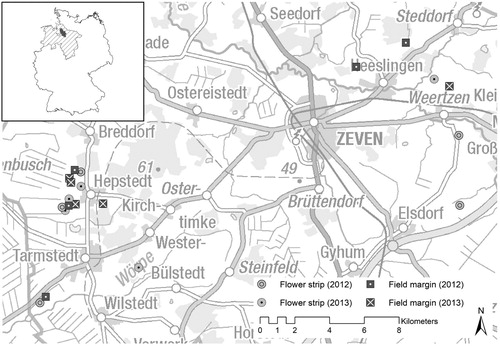
We investigated: (a) five flower strips representing flower-rich and highly structured habitats and (b) five field margins characterized by the dominance of grasses and by a low to medium structural diversity. All sites were located between maize fields and unsealed farm tracks. All flower strips were 6 m wide, the width of the field margins varied from 1 to 5 m. The flower strips examined in the winter of 2012 were sown with the seed mixture ‘Rotenburger Mischung 2012’, all the other flower strips were sown with ‘Rotenburger Mischung 2013’. These seed mixtures differed slightly in terms of species composition and seeding rate (online Table S1).

Survey methods

We conducted bird surveys using camera trapping and line transects in the winters of 2012/13 and 2013/14, summer of 2013 and autumn of 2013 (Table 1). In total, the cameras were exposed 15 times on each flower strip and 15 times on each field margin. Line transects were carried out 65 times on each flower strip and 57 times on each field margin. In the first winter, we did not conduct line transects in field margins. In order not to disturb the camera trapping with our presence, we conducted the line transects on the following day.

Table 1. Sampling design in the different seasons of the years 2012–2014. V: total number of visits (line transects); Cd: total number of camera-days (camera trapping); n: number of study sites (flower strips and field margins); Winter 2012/13 no surveys on field margins by line transects.

Winter 2012/13			Summer 2013			Autumn 2013			Winter 2013/14
Period	V n = 5	Cd n = 10	Period	V n = 10	Cd n = 10	Period	V n = 10	Cd n = 10	Period	V n = 10	Cd n = 10
06/01–14/01	15	10	30/06–08/07	50	10	26/09–30/09	50	10	02/12–10/12	50	10
09/02–13/02	10	10	24/07–29/07	40	10	16/10–20/10	50	10	17/12–21/12	50	10
14/02–18/02	15	10	09/08–13/08	40	10	30/10–03/11	50	10	21/01–25/01	50	10
			14/08–22/08	40	10	19/11–23/11	50	10	20/02–25/02	50	10
Total	40	30	Total	170	40	Total	200	40	Total	200	40

We attempted to identify birds to species level but if a bird could not be identified to species, we documented the family or classified the bird depending on its body size. We distinguished between small-sized unknown birds (like finches), medium-sized unknown birds (like Blackbirds Turdus merula) and large-sized unknown birds (like pigeons).

Camera trapping

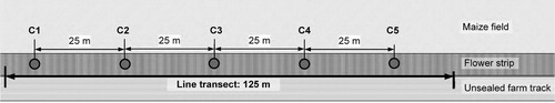
We used the ‘Dörr SnapShot Extra 5.0’ camera model because its time-trigger function can be programmed at intervals to the second and can be used independently of the passive infrared-sensor (PIR-sensor). In this study, we programmed still images to be taken at 20 s intervals, with the PIR-sensor in ‘off’ status. We exposed five cameras per study site, in a row, with a distance of approximate 25 m between each camera (Figure 2). For installation of the camera traps, ground sleeves were permanently anchored in the ground (online Figure S1). This enabled quick set up of the cameras (approximately 25 min for the five cameras per study site), and ensured identical recording points throughout the investigation period. We installed the cameras 70 cm above the highest vegetation layer at each study site, using metal rods. The camera angle was adjusted by a wedge of polystyrene between the rod and the camera (online Figure S2). This was done so that we could determine a recording area. Laterally, the recording area was limited by the width of the flower strips or the field margins. Image depth varied depending on the camera angle and the vegetation height. The daily adjusting of the camera angle made it possible to ensure an image depth of a minimum of 6 m in all cases. Due to the in-built display, image viewing on-site was feasible as was the controlling and correcting of the camera angle and the recording area.

Figure 2. Diagram of the research design (C1–C5: 5 camera locations).

During one sampling period, the cameras were installed for one day on each study site from early morning (around 07:30) until evening (around 17:00). According to the season, exposure time ranged from 8 to 11 h. To analyse the data, we defined a camera day as one day on which the five cameras were operational in the field on one study site. Each study site was examined once per round for each season (Table 1).

Line transects

Along the camera locations, we also conducted line transects on a length of 125 m, recording all bird sightings (Figure 2). In order to obtain a data structure comparable to the camera traps, the number of species was defined by the total number of bird species discovered per round during different visits to the same study site. We only counted birds sitting on the ground, in the vegetation and those flying into or out of the transect. Birds flying across the study sites were not recorded unless they were searching for food on the study sites. The line transects were carried out between sunrise and early evening, corresponding to the camera trapping. For each season, each study site was examined two to five times per round (Table 1). In order to avoid bias due to time of day or weather, we changed the order of visiting the study sites each day and all observations were only conducted during suitable weather conditions (Bibby et al. 1992).

Data preparation: camera trapping

Screening the photographic material

The images were evaluated manually. Analysing a sequence of images in fast motion enabled a good detection of birds. Watching the images as a relatively fast sequence allowed the detection of small-sized birds much more easily than looking at single images. Only pictures where the bird could be identified clearly as a bird were included in the analyses. Furthermore, the bird had to be into the defined recording area.

A sequence of images with continuous bird records was regarded as one ‘presence time’. As soon as the bird moved out of the camera’s field of view, the presence time was considered to be over, even if the bird came back later. In this case, a new presence time began.

Exposure time and presence frequency

Due to the variation of exposure time, caused by different day lengths during the different times of the year, a time-based standardization was necessary for comparing the data. The exposure time of each study site was calculated by the mean of all camera days per season and the mean of the five cameras of each study site.

In the same way, we generated the presence frequency of the species. The presence frequency is given in minutes in relation to 100 h of exposure time, hereafter simply referred to as ‘presence frequency (min)/100 (h)’ or just ‘presence frequency’.

Throughout the investigation period, camera errors occurred in seven cases, either affecting a whole day of recording or several hours. In addition, there were individual defective images due to technical problems or weather conditions (overexposure due to backlight of the sun), which accounted for only about 0.5% of the total recording time.

Time of day

We calculated the number of days on which birds occurred at a specific one-hour interval of the day. A species was only counted once for each period of time and each study site, regardless on which of the five ranged cameras the species was recorded. Additional records of the same species at the one-hour interval and in the same study site was not taken into account. Unknown birds or species, which were defined at family level, were only counted if there was no observation of a species of the same body size or family on the study site and period before. At certain one-hour intervals, the cameras were used with varying frequency due to differences in day length. Therefore, the number of days with birds was standardized in relation to the number of days the cameras were set up in the field.

Statistical analyses

Statistical analyses for method comparison focused on the number of species as a comparable unit of measurement between the two methods. Since repeated measures were performed in this study, statistical analyses were calculated with linear mixed-effects models to determine the effect of habitat type, season and method.

Response variables, explanatory variables and random effects

The total number of recorded bird species (as a proxy for species richness, defined by the total sum of recorded species per round) was used as the response variable (Table 2). Three explanatory variables were included in the analyses: habitat type, season and method (Table 2). Study sites were examined repeatedly in different seasons. Without further criteria, they cannot be considered as independent variables. The season was used as one variable to define independent data. In addition, as the birds were recorded on blocked dates and against the background of phenological changes, the consecutive dates (defined as rounds) must be considered in the statistical analyses. Therefore, we regarded one study site for each round of the respective season as one unit of analysis (sample size: winter 2012/13 n = 15, summer 2013 n = 20, autumn 2013 n = 20, winter 2013/14 = 20). For the data structure of the random-effects, we therefore chose variance of the study site, the interaction of study site and season as well as the interaction of study site, season and round: (1|site) + (1|site:season) + (1|site:season:round) (Table 2).

Table 2. Overview of the response variables (resp), explanatory variables (expl) and random effects (ran).

Variable	Description
Species (resp)	Total number of recorded bird species by using different methods (camera trapping: CT, line transects: LT) and combination of these methods (MC = CT or LT). It was defined by the total sum of recorded species of each study site and each round per season.
Season (expl and ran)	Season in which the investigations were carried out: Winter 2012/13 (wi12), summer 2013 (su13), autumn 2013 (au13) and winter 2013/14 (wi14)
Habitat type (expl)	Two different habitat types were investigated: Flower strips (FS) and field margins (FM)
Method (expl)	Applied method to record birds. CT = Camera trapping, LT = Line transects, MC = method combination (CT or LT)
Study site (ran)	Name of the study site
Round (ran)	The birds were recorded on blocked dates. The blocked appointments were summarized in time as rounds of 5–9 days (Table 1).

Linear mixed-effects models

Three different datasets were used: Dataset 1 included both habitat types, dataset 2 the flower strips and dataset 3 the field margins. Since the field margins were not investigated by line transects in the winter of 2012/13, this season was excluded from dataset 1 and 3. In dataset 1, the number of species recorded by line transects and the number of species recorded by camera traps were compared. In dataset 2 and 3, the two methods were also analysed in comparison to the combination of both methods (sum of number of species recorded by line transects or camera traps).

In line with current scientific knowledge for Poisson-type count data, which incorporates random effects, the generalized linear mixed model (GLMM) was applied (Bolker et al. 2009). Single models were run with GLMM, but when adding interactions between the fixed-effects, the GLMM model failed to converge (online Table S2).

As the GLMM was not stable for our data sets, we used linear mixed-effects models (LMM). For model comparison the LMMs were fitted by maximum likelihood (ML) estimations, for further analyses by restricted maximum likelihood (REML; Zuur et al. 2009). The number of species was log-transformed (log(y + 1)) to meet the assumption of normally distributed data (residuals and random-effects). Time-correlated measurements for the time series of the individual study sites were assumed (corAR1-structure). For model comparison, likelihood ratio tests (LRT; Bolker et al. 2009, Zuur et al. 2009) and corrected Akaike information criterion (AICc) were used (Burnham & Anderson 2002). The confidence interval (CI) was calculated with a 95% CI for the final LMMs. Pairwise comparisons of the mean values between habitat type, method and/or season were performed on the basis of model estimators and adjusted for multiple comparisons analogous to the Tukey test. The assumptions (homoscedasticity, normality of residuals and random-effects) were tested by residual plots and Q-Q plots. No notable violations were detected.

Analyses were calculated in the R language and environment (R Core Team 2017, RStudio Team 2016). For GLMM the Package ‘lme4’ (Bates et al. 2015) was used, and for linear mixed-effect models the package ‘nlme’ was used (Pinheiro et al. 2018). AICc values were calculated with the package ‘MuMin’ (Kamil 2018) and pairwise comparisons with the ‘lsmeans’ package (Lenth 2016). The figures were created with ‘ggplot2’ in R (Wickham 2016) or in IBM SPSS Statistics 25.

Results

Method comparison: camera trapping versus line transects

Bird communities

Over the entire study period, we observed 26 bird species (Table 3). Of these, 20 were recorded during the entire 150 camera-days (1,227,794 images, including 3902 showing the presence of birds). During the 610 site-inspections by line transects we also detected 20 species.

Table 3. Comparison of the two survey methods with regard to species range and species numbers. CT: Camera trapping, LT: Line transect, ^asmall-sized songbirds, ^bgalliformes, grey highlights: species recorded by both survey methods (CT and LT).

		Flower strips								Field margins								Entire investigation period
		Winter 2102/ 13		Summer 2013		Autumn 2013		Winter 2013/ 14		Winter 2102/ 13		Summer 2013		Autumn 2013		Winter 2013/ 14		Flower strips		Field margins		Total
Scientific name	English name	CT	LT	CT	LT	CT	LT	CT	LT	CT	LT	CT	LT	CT	LT	CT	LT	CT	LT	CT	LT	CT	LT
Alauda arvensis^a	Skylark			x					x		not inspected by line transects		x	x				x		x		x
Ardea cinerea	Grey Heron													x						x		x
Carduelis carduelis^a	Goldfinch					x									x			x			x	x
Chloris chloris^a	Greenfinch	x			x	x			x									x				x
Columba palumbus	Woodpigeon			x														x				x
Corvus corone	Carrion Crow															x				x		x
Corvus frugilegus	Rook											x								x		x
Coturnix coturnix^b	Quail					x		x										x				x
Cyanistes caeruleus^a	Blue Tit							x										x				x
Emberiza citrinella^a	Yellowhammer				x		x	x				x					x	x		x		x
Fringilla coelebs^a	Chaffinch	x					x		x						x			x			x	x
Hirundo rustica/Delichon urbicum^a	Swallow/House Martin			x														x				x
Lanius collurio^a	Red-backed Shrike												x								x		x
Motacilla alba^a	Pied Wagtail			x														x				x
Motacilla flava^a	Yellow Wagtail			x			x					x			x			x		x		x
Parus major^a	Great Tit		x		x	x			x									x				x
Passer montanus^a	Tree Sparrow			x			x		x			x			x		x	x		x		x
Phasianus colchicus^b	Pheasant	x		x		x		x										x				x
Phylloscopus collybita^a	Chiffchaff				x								x						x		x		x
Phylloscopus trochilus^a	Willow Warbler						x												x				x
Pyrrhula pyrrhula^a	Bullfinch		x	x			x											x				x
Saxicola rubicola^a	Stonechat			x								x		x				x		x		x
Sylvia borin^a	Garden Warbler				x														x				x
Sylvia communis^a	Whitethroat			x			x					x						x		x		x
Troglodytes troglodytes^a	Wren								x										x				x
Turdus merula	Blackbird						x												x				x
Fringillidae^a	Finch					x			x									x				x
Small-sized unknown birds^a		x		x		x		x				x		x		x		x		x		x
Medium-sized unknown birds				x														x				x
Large-sized unknown birds			x																x				x
Number of species recorded with the combination of methods (CT or LT)		5		15		13		10				9		7		4		22		13		26
Number of species recorded with both methods (CT and LT)		3		7		3		2				2		1		0		14		4		14
Number of species only recorded with CT		0		3		2		2				4		2		2		3		5		6
Number of species only recorded with LT		2		5		8		6				3		4		2		5		4		6

Concerning the bird communities, the two methods led to different results. Throughout the entire investigation period and for both habitat types, only about half of the recorded species were recorded by both methods (14 species, Table 3). When comparing the camera trapping results to those of the line transects, we noticed six additional species in each case: Carrion Crow Corvus corone, Quail Coturnix coturnix, Woodpigeon Columba palumbus, Blue Tit Cyanistes caeruleus, Grey Heron Ardea cinerea and Rook Corvus frugilegus were only recorded by camera trapping, while the Chiffchaff Phylloscopus collybita, Blackbird, Garden Warbler Sylvia borin, Wren Troglodytes troglodytes, Red-backed Shrike Lanius collurio and Willow Warbler Phylloscopus trochilus were only recorded by line transects.

In flower strips, various species were detected by both methods (14 species, Table 3). We recorded more additional species by using the line transects method (five further species: Chiffchaff, Blackbird, Garden Warbler, Wren and Willow Warbler) than by using camera traps (three further species: Quail, Woodpigeon and Blue Tit). In field margins, however, the reverse was the case. Only a small number of species were recorded by both methods (4 species, Table 3). We observed five species exclusively by using camera traps (Carrion Crow, Stonechat Saxicola rubicola, Whitethroat Sylvia communis, Grey Heron and Rook) and four species (Chaffinch Fringilla coelebs, Chiffchaff, Goldfinch Carduelis carduelis and Red-backed Shrike) solely by using line transects.

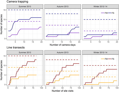
The species accumulation curves show that the saturation limit in flower strips was better reached in all seasons by using line transects than by using camera traps (Figure 3). In the field margins, however, the two methods were very similar. With camera trapping, the maximum number of species was reached in summer after only a few camera-days, both in the flower strips (after 6 camera-days) and in the field margins (after 8 camera-days). In autumn, however, the number of species in the flower strips did not increase significantly until the end of the observation period (after 14 camera-days). In most cases when using line transects, the number of species hardly increased after approximately 60–70 site visits. In surveys with overall low bird counts (camera traps: autumn and winter, flower strips and field margins; lines transects: winter, field margins), the number of species increased only slowly over the entire investigation period.

Figure 3. Number of species in relation to research effort. Broken line represents 100% of the overall number of detected species (by both methods) for each habitat type (FM = Field margins, FS = Flower strips). Camera trapping: Each camera day of one of the five study sites of each habitat type was calculated as an individual camera-day. Line transects: Each visit of one of the five study sites of each habitat type was calculated as an individual visit.

Effect of habitat type, applied method and season on number of bird species

Testing the three variables ‘habitat type’, ‘method’ and ‘season’ (and their interactions) in different model comparisons (online Table S3) revealed that the model which included the interaction between habitat type and method, as well as the additional effect of the season, best described the number of species recorded.

The model calculations resulted in significantly fewer species in field margins than in flower strips (16–38% less on average over the levels of method and season, 95% CI; Table 4 (a): FM-FS). Averaged over the levels of habitat type and season, the number of species recorded by camera trapping was significantly lower than the number of species recorded by line transects (decrease by 5–23%, 95% CI; Table 4 (a): CT-LT). The differences between the habitat types were more pronounced when using line transects than when using camera traps. With line transects, on average, 24–48% fewer species were recorded in field margins than in flower strips. When using camera traps in field margins, the species number remained constant or decreased by 32% compared to flower strips (Table 4 (a): CT/ LT: FM – FS).

Table 4. Pairwise comparison of the mean number of species between the habitat types and/or the applied method and/or the season for (a) both habitat types (lsmeans to lme2 fitted by REML, selected contrasts) (b) flower strips (lsmeans to mod6 fitted by REML) and (c) field margins (lsmeans to mod8 fitted by REML). As the season had no significant effect on number of species in flower strips (b), no seasonally specific analyses were carried out for this habitat type. Results are given on the log (not the response) scale; only Confidence-Intervals (CI) are back-transformed from the log scale. FS: Flower strips; FM: Field margins; CT: Camera trapping; LT: Line transects; MC: Method combination.

Contrast		Estimate	se	Df	t	P	CI (95%)
(a) Both habitat types together
	FM – FS^a	−0.3276409	0.0645235	8	−5.078	0.0010	0.62	0.84
	CT – LT^b	−0.1582613	0.0520862	118	−3.038	0.0029	0.77	0.95
	CT: FM – FS^c	−0.1944475	0.0829232	8	−2.345	0.0471	0.68	1.00
	LT: FM – FS^c	−0.4608342	0.0829232	8	−5.557	0.0005	0.52	0.76
(b) Flower strips
	CT – LT^d,e	−0.273107	0.060400	148	−4.521639	0.0000	0.66	0.88
	MC – CT^d,e	0.455696	0.054796	148	8.316227	0.0000	1.39	1.80
	MC – LT^d,e	0.182589	0.060400	148	3.022997	0.0083	1.04	1.38
(c) Field margins
	CT – LT^d,e	−0.02507	0.04662	114	−0.53776	0.8529	0.87	1.09
	MC – CT^d,e	0.16370	0.03635	114	4.50371	0.0000	1.08	1.28
	MC – LT^d,e	0.13863	0.04662	114	2.97389	0.0100	1.03	1.28
su13	CT – LT5^e	0.06343	0.08074	114	0.78555	0.7127	0.88	1.29
su13	MC – CT^e	0.15890	0.06296	114	2.52406	0.0344	1.01	1.36
su13	MC – LT^e	0.22233	0.08074	114	2.75362	0.0187	1.03	1.51
au13	CT – LT^e	−0.20794	0.08074	114	−2.57547	0.0301	0.67	0.98
au13	MC – CT^e	0.26287	0.06296	114	4.17558	0.0002	1.12	1.51
au13	MC – LT^e	0.05493	0.08074	114	0.68034	0.7754	0.87	1.28
wi14	CT – LT^e	0.06931	0.08074	114	0.85849	0.6675	0.88	1.30
wi14	MC – CT^e	0.06931	0.06296	114	1.10102	0.5154	0.92	1.24
wi14	MC – LT^e	0.13863	0.08074	114	1.71698	0.2033	0.95	1.39

^aResults are averaged over the levels of: method, season.

^bResults are averaged over the levels of: habitat type, season.

^cResults are averaged over the levels of: season.

^dResults are averaged over the levels of: season.

^eP value adjustment: Tukey method for comparing a family of 3 estimates.

Effect of applied method and season on number of bird species

Testing the effect of the two variables ‘method’ and ‘season’ (and their interactions) in different model comparisons (online Table S4) revealed that the model which included the method and the additional effect of the season best described the number of recorded species in flower strips. With regard to the field margins, the model that took into account the interaction between the method and the season turned out to be the most suitable.

Averaged over all seasons, the different methods had a highly significant influence on the number of species in flower strips (Table 4(b)). Using camera traps for counting birds led to significantly fewer species than using line transects (on average 12–34% less, 95% CI). The combination of methods compared to camera trapping led to a highly significant increase in the number of species by an average of 39–80% (95% CI). The combination of methods also allowed the recording of significantly more species than the line transects alone. However, the increase was distinctly lower (4–38% on average over the seasons, 95% CI). The seasons had no significant effect on the number of species in flower strips, which is why this result can be applied to all seasons investigated.

In contrast to flower strips, the number of species recorded by line transects in field margins did not differ significantly from the number of species recorded by camera trapping (averaged over the level of seasons, Table 4(c)). Therefore, the comparison between the combination of both methods and the two individual methods showed a similar increase in the number of species (increase by 3–28% or 8–28%, 95% CI). The seasonal analysis for the field margins revealed that the significant differences only occurred in the summer of 2013 and the autumn of 2013, but not in the winter of 2014. The results of the summer are in line with the overall results. In autumn, however, a significant difference between line transects and camera traps could be detected: when using camera traps significantly fewer species could be recorded than when using line transects (decrease by 2–33%, 95%CI).

Presence frequency

In flower strips, we observed the Pheasant Phasianus colchicus by using cameras with a very high average presence frequency and with a clear distance to all the other detected species (online Table S5). This was the only species recorded in flower strips during all seasons. The next highest average presence frequencies by camera traps were documented for Greenfinch Chloris chloris. In the case of line transects, however, the Pheasant was only rarely observed (online Table S6). With the line transects, Greenfinch were most frequently observed, followed by Yellow Wagtail Motacilla flava and Yellowhammer Emberiza citrinella.

In field margins, Carrion Crow and Yellow Wagtail were the most frequently recorded species by camera traps (online Table S5). The latter was also observed frequently by line transects and only the Yellowhammer was observed more frequently (online Table S6).

Camera traps: technical and additional ecological information

Presence time and time intervals of the camera trigger

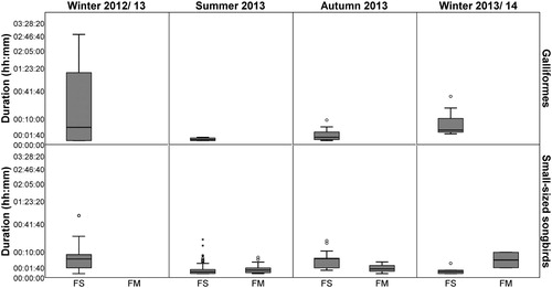
Long bird occurrences in front of the camera were rare, especially in the field margins (Figure 4; to make the short presence times recognizable, the y-axis is shown with power-scaling). The longest presence time was nearly three hours and only one other record lasted over two hours; both were occurrences of Pheasants and were observed in flower strips in the winter of 2012/13. The longest presence time of small songbirds took nearly one hour and it was also observed in a flower strip in the winter of 2012/13. However, most of the birds stayed just a short while in front of a camera. The presence time of half of the bird observations took less than one minute. One-third of the records were captured by only one photo, representing a presence time which lasted only a maximum of 20 s. The Mann–Whitney U test showed no significant differences.

Figure 4. Presence time of birds in front of a camera. The calculation is based on the time-triggered interval of 20 s. One picture with bird occurrences was counted as a presence time of 20 seconds. For a better representation of the short presence times the y-axis was power-transformed. FS = flower strips (galliformes: winter 2012/ 13: n = 8, summer 2013: n = 4, autumn 2013: n = 7, winter 2013/14: n = 12; small-sized songbirds; winter 2012/ 13: n = 0, summer 2013: n = 48, autumn 2013: n = 3, winter 2013/14: n = 2), FM = field margins (galliformes: all seasons n = 0; small-sized songbirds: winter 2012/13: n = 34, summer 2013: n = 59, autumn 2013: n = 13, winter 2013/ 14: n = 5), n = number of bird observations, ° = outliers (cases whose values are 1.5 to 3 times the height of the boxes), * = extreme outliers (cases whose values are more than three times the height of the boxes).

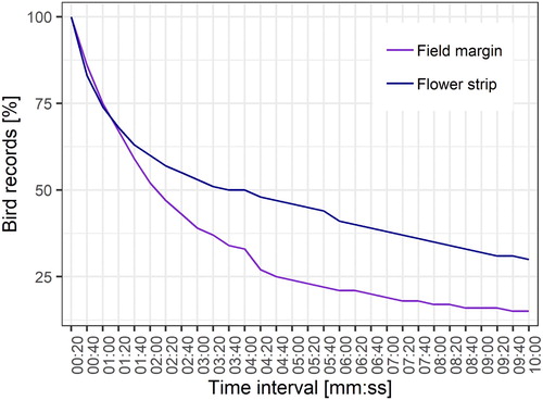
For the analysis of the optimal interval for the camera trigger, the probabilities of the bird detections were calculated as a function of the duration of the bird occurrence and the increase of the time interval: The 20 s interval used in our study was regarded as the baseline at which all bird detections were recorded. Assuming a 40 s interval, bird detections of 20 s presence time could only be recorded to 50%, all longer bird detections to 100%. At a 60 s interval, bird detections of 20 s presence time could be recorded at 33.33%, bird detections of 40 s presence time at 66.66%, and all longer bird detections at 100%, and so on. A slight increase in the time interval from 20 to 40 s led to approximate 15% fewer bird records (Figure 5). Increasing the time interval from 20 s to one minute reduced the number of bird recordings by approximate 25%. For a time interval of up to one minute and 20 s, the decrease in bird records on flower strips and field margins was similar. After this time, the bird records on the field margins decreased more strongly than on the flower strips. Hence, only 50% of the bird occurrences were recorded in the field margins at an interval of two minutes. In the flower strips this occurred at an interval of three minutes.

Figure 5. Number of detected bird occurrences as a function of the time interval of the camera trap trigger. Percentage of bird records were calculated per habitat type (flower strips n = 159, field margins n = 63).

Time of day

The number of days with bird records in relation to the number of camera days at different times of day was similarly high across all seasons in the flower strips and the field margins. In the flower strips, the detection rate in the early morning (05:00–08:00) was 30%, in the afternoon (15:00–18:00) 10% (on average per one-hour interval). In the field margins, the proportion was 10% at both times of the day.

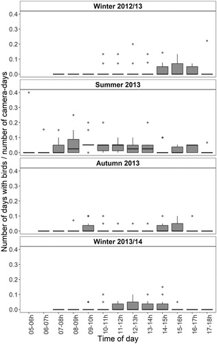
In the winter of 2012/13, the first records of birds occurred at 10:00 in the morning and most of the birds were recorded between 14:00 and 17:00 (Figure 6). In the winter of 2013/14, the records of birds occurred earlier. In this season, bird observations accumulated between 11:00 and 15:00 and the Friedman test showed significant differences between avian observations and the time of day (χ² = 19.856, P = 0.031, n = 10). However, the subsequent post-hoc test did not reveal any significant differences between the individual time of day. In the summer, birds were recorded throughout the day, with a peak at between 7:00 and 14:00. In the autumn, birds were recorded both at midday and in the afternoon, peaking at between 8:00 and 11:00 and at between 14:00 and 17:00.

Figure 6. Temporal pattern of bird occurrence in different seasons of the year. Presented as percentage of the number of days with birds (days with birds present at the specific time of day) to the number of camera-days (days on which camera traps were operational in the field at the one-hour interval).

Presence frequency

In summer, small-sized songbirds were regularly recorded in flower strips at different seasons as well as in field margins (online Table S5). However, only in the winter of 2012/13 was a high presence frequency of small-sized songbirds (notably Greenfinch and unknown small birds) recorded on flower strips. And only in this season were the presence frequencies in flower strips (median = 42.6) significantly above the presence frequencies in field margins (median = 0; Mann–Whitney U test: P = 0.025). Otherwise, the median was very low and high presence frequencies were only documented on single study sites as extreme values.

Galliformes were only observed in flower strips and mainly in winter (online Table S5). However, here too, the high presence frequencies were extreme values and were due to the occurrence of the Pheasant on single study sites, especially in the winter of 2012/13. Quail were observed much less often. All other birds (Carrion Crow, Woodpigeon, Blackbird, Grey Heron and Rook) were only recorded as low numbers of individuals.

Discussion

Advantages and limits of a multi-method approach

Advantages

The results clearly demonstrate that combining camera trapping with traditional bird census methods provides a decisive advantage. First of all, considering the entire investigation period and both habitat types together, we observed as many species by lots of short visits (using line transects) as by a few multi-hour observations (using camera traps). However, the bird communities varied depending on the method used. By applying the combination of methods, we recorded about 25% more species, and each additional method increased the species richness by about 25% (over the entire investigation period and in both habitats together). With regard to the frequencies of the species, the two methods also led to different results. Furthermore, the results of the linear mixed-effect models show that significantly more species could be detected by the multi-method approach than by one method alone. On the basis of our data, it could not be clarified whether the intensification of one method would have resulted in the same increase in number of species as the combination of the two methods. Carrying on from this, further comparative studies are required. Our analyses for estimating the overall coverage of all species, however, indicated that intensifying one method seems not to be as favourable as combining both methods. In many instances when using line transects, the number of species stagnated after around 60–70 visits. In addition, with 75–100 line transects per season, this method was carried out very intensively in our study. Furthermore, we did not identify any systematic differences (bias) in the bird communities. Neither method was capable of recording species that the other was unable to due to ecological or biological reasons e.g. for large, rare or ground-dwelling species (Dinata et al. 2008, O’Brien & Kinnaird 2008). In our study, the differing bird communities were due rather to principal differences between the two methods: camera traps allow substantially longer observation times than line transects. The camera recordings of our survey represents 1360 field observation hours at five locations per study site (achieved over a 20 s interval). In comparison, by using line transects, the study sites were observed for only 220 h. On the other hand, line transects are characterized by a high number of repetitions. The line transects were repeated 65 times, whilst the camera traps were only repeated 15 times. In addition, a larger continuous area can be observed by line transects (125 m) than by camera traps (at least approximately 30 m; camera section approximately 6 m deep at five camera positions).

Furthermore, the models and species accumulation curves demonstrated that habitat type and method had a decisive influence on bird detection. Therefore, the extent of the advantage of multiple methods mainly depends on both the habitat type and the method used. In flower strips, the use of line transects led to significantly more species being detected than the use of camera trapping. Accordingly, the combination of methods only provided a small additional profit and in flower strips, line transects were more beneficial than camera traps. On the other hand, in field margins, the method had no significant influence on the number of species detected. In this case, both methods contributed equally to the advantage of the combination of methods which is very beneficial in this habitat type.

The influence of the seasons on the number of species detected in field margins may not be as important as indicated by the linear mixed-effect models. The seasonal differences in this habitat type are more due to the low number of species detected in the winter of 2012/13, which was the only season without significant differences. Both with using line transects and with using camera trapping, only very few species (two species each) were observed in field margins during this season (both methods: median = 0). Therefore, no significance could be extrapolated. However, since different species could be observed with each method, the combination of methods proved to be advantageous in winter as well. Since the number of species is too small to make clear recommendations as to whether camera trapping or line transects are better for certain seasons, there is a need for further research.

Technical demands for using time-triggered cameras

Our study documented that short intervals are a determinant for the use of time-triggered cameras to survey birds. The majority of the recorded species were only captured on one to three photos, which is equivalent to a maximum stay duration of 20 s to 1 min. In addition, it could be demonstrated that even a small increase in the camera trigger interval from 20 s to 40 or 60 s leads to considerable data loss. Other studies operating with time-triggered camera traps also show that long intervals between each recorded image result in substantial information loss or misrepresentation (Hamel et al. 2013, Huffeldt & Merkel 2013). They used time-triggered camera traps with much larger intervals than we did (5 min versus 20 min intervals (Hamel et al. 2013), 1 to 5 h interval (Huffeldt & Merkel 2013)). At this point, the different research topics and target groups have to be considered. Huffeldt & Merkel (2013) collected population parameters at seabird colonies for the duration of the breeding season in Greenland. Hamel et al. (2013) studied avian and mammalian scavengers at baited sites in subarctic/arctic tundra. In this way, a continuous and regular presence of animals over a long period of time, in front of the camera, was guaranteed in both of these studies. Our results showed that a short interval of under one minute is required for recording birds in semi-natural habitats in the agricultural landscape, in habitats where birds stay only for a short time and just occasionally. This also applies to rare or cryptic species or to study sites and seasons with low bird density. Hamel et al. (2013) also highly recommend a short time interval (1 min) or even video cameras for recording raw detections.

Furthermore, a high number of camera days and a long exposure time of camera traps on different study sites are necessary. We only recorded high presence frequency as extreme values on single study sites. On most study sites the presence frequency was low and so the presence frequencies varied widely. Moreover, the number of species observed in the autumn did not increase until the end of the survey period.

Assessment of the advantages and limits

The technical demands (short intervals, high number of camera days and a long exposure time of camera traps) form the essential basis for the recording of valid and reliable data when using time-triggered cameras. Together, these requirements show the limit of time-triggered cameras: the high data volume. First, it is difficult to manage (the storage or back-ups, sharing and analyses of the recordings (Huffeldt & Merkel 2013)). The recordings of our study encompassed 1,227,794 images with a data volume of approximately 2.6 terabytes. But above all, the viewing of the images is very time-consuming. Viewing the images combined as a video of approximately 30 min covers a total field recording time of 375 h of recordings but is multiplied up by ten study sites each with five cameras and 15 repetitions. On the other hand, the field work with camera traps (about 100 h in total for set up and removing) was only half as time-consuming as the field work with line transects (about 220 h in total). For camera trapping, the daily reading of the memory cards (10 min per memory card) was also required and amounted to a total of about 125 h. Thus, the survey by camera traps was altogether about three times as time-consuming as the survey by line transects, whereby the evaluation of the recordings represented a substantial part. As far as our experience goes, this is the major limiting factor concerning time-triggered camera trapping. At this point, however, several positive aspects take effect. First, viewing the recordings can be conducted independently of time and space, and are weather- and researcher-independent. Furthermore, the camera traps work autonomously in the field and high observation durations are possible without the need of researchers at the study sites. In our study, we could conduct other surveys (line transect surveys of birds as well as vegetation surveys) while the camera traps were active in the field. Additionally, when using camera traps, the study sites are absolutely undisturbed, with no human interference in the area. Depending on the study design, there could be ways to reduce the image material, for example by increasing the interval from 20 to 40 s but this comes at the potential cost of lost detections, as discussed above. Moreover, knowing the daily activity pattern of the target species is helpful to determine the optimal recording time in order to save time. Our results showed that certain hours of camera trapping in the morning as well as in the evening could be saved. Especially in long-term studies with a high number of camera days, the daily saving of a few hours has a considerable effect on the effort.

Ecological aspects for using camera trapping

Time of day

Our study shows that camera trapping can be used to investigate the diurnal activity pattern of birds. The results demonstrate a peak of bird records in the morning in summer. However, our studies indicate that bird surveys in winter must not necessarily be carried out during the morning hours. In this season, the period from early noon to afternoon is particularly suitable. During autumn, bird surveys can be conducted at any time of the day. The available data does not suffice for transferable or general recommendations, as bird activity and detectability is very weather dependent and can seriously affect the effectiveness of surveys. There is a need for further research on this issue which should be further investigated when using camera traps.

Estimating bird abundance

The number of individuals can be counted on the basis of the images from the camera traps. However, it is not possible to verify whether new individuals actually appear in the photo series or whether the same individuals appear repeatedly. But if the birds can be marked or if individual identification is possible, the abundance can be estimated and capture–recapture studies can be conducted. In addition, O’Brien & Kinnaird (2008) developed a model to estimate abundance when individual identification is not possible.

Conservation value of semi-natural habitats

The number of recorded species in flower strips was significantly higher than the one in field margins, independent of the applied method or the season. Furthermore, small-sized songbirds used flowers strips much more intensively than field margins, in summer and in autumn as well as in the first winter. In addition, Pheasant and Quail were never recorded in field margins. These results clearly show that flower strips provide a positive contribution to biodiversity (Aschwanden et al. 2005, Buner et al. 2005).

Especially in winter, there is a striking lack of cover and food in cleared, intensively used agricultural landscapes (Moorcroft et al. 2002, Gillings et al. 2005, Siriwardena et al. 2008). Also in winter, a high presence frequency and a long presence time of birds in flower strips could be recorded by camera trapping. Hence, flower strips can improve the availability of food and cover (Wagner et al. 2014, Wix & Reich 2018).

Practical advice on the use of time-controlled camera traps: mounting and equipment safety

With multiple cameras in relatively small areas, there is considerable potential for expensive losses of equipment. Even more critical, depending on the duration of the camera exposure, is the high data loss. In the open agricultural landscape, however, equipment and data safety is difficult as there are no trees or comparable structures to which the cameras can be fixed and locked. Therefore, it was necessary to remove the camera traps every evening. Due to the permanently installed ground sleeves, the setup and removal of the cameras was not so time-consuming (setup and adjustment of one camera took about 5 min, removal about 3 min). In our study this effort payed off: none of the camera traps were stolen or damaged. In addition, the quick setup of the camera traps kept the disturbance of the study sites, during the setup process, to a minimum.

Conclusions

In summary, it can be stated that multi-method studies are recommended to record bird communities more reliably. The combination of methods was particularly beneficial in study sites with low bird densities and bird activity, such as in the field margins. Line transects and camera trapping are equivalent methods in such habitats with regard to the number of recorded species. This supports the results of Dinata et al. (2008) suggesting the use of camera traps for difficult to detect rare species, which is comparable with a situation of low bird activity or density. On the other hand, line transects were much more advantageous in study sites with high bird densities and bird activity such as in flower strips. In these habitat types, the use of camera traps cannot replace traditional bird census methods. Pirie et al. (2016), who conducted a method comparison (camera traps versus dung detections) to mammals in savannah, also concluded that the use of camera traps cannot replace surveys with experienced researchers in field. The additional workload of a multi-method approach must also be in proportion to the additional profit. In habitats with high bird activity, camera traps are not as beneficial as in habitats with low bird activity.

The combination method of camera traps and traditional bird census methods is limited mainly by the high expenditure of time needed for screening the recordings of the camera traps. Automated image (and sound) recognition, however, is a rapidly evolving field and the continuous development is promising. There are already programmes for managing large amounts of image data and facilitating analyses (Fegarus et al. 2011, Krishnappa & Turner 2014, Bubnicki et al. 2016, Niedballa et al. 2016). Moreover, there are software-packages to semi-automatically identify the occurrences of medium- to large-sized animals (Adams et al. 2006, Raj et al. 2015, Price Tack et al. 2016) which can reduce the time required to evaluate the recordings. In addition, a continuous improvement of the image quality can be assumed, whereby it is possible to better identify small birds. Hence, due to technical developments, the use of camera traps to record birds has a very promising future. This is of particularly interest as camera traps can be used to obtain further information such as presence time, presence frequency and time of day in addition to the number of species.

Acknowledgements

We are grateful to Dr L. von Falkenhayn for proofreading the English manuscript. We thank the farmers for providing access to their land. We thank the reviewers for their constructive feedback. We are also grateful to the Lower Saxony Ministry of Food, Agriculture and Consumer Protection for the financial support of this study.

ORCID

Nana Wix http://orcid.org/0000-0002-3371-040X

Additional information

Funding

This work was supported by the Lower Saxony Ministry of Food, Agriculture and Consumer Protection [105.1-3234/1-5(267)].

References

- Adams, J.D., Speakman, T., Zolman, E. & Schwacke, L.H. 2006. Automating image matching, cataloging, and analysis for photo-identification research. Aquat. Mamm. 32: 374–384. doi: 10.1578/AM.32.3.2006.374
- Ahumada, J.A., Hurtado, J. & Lizcano, D. 2013. Monitoring the status and trends of tropical forest terrestrial vertebrate communities from camera trap data: a tool for conservation. PloS one 8: e73707. doi: 10.1371/journal.pone.0073707
- Aschwanden, J., Birrer, S. & Jenni, L. 2005. Are ecological compensation areas attractive hunting sites for common kestrels (Falco tinnunculus) and long-eared owls (Asio otus)? J. Ornithol. 146: 279–286. doi: 10.1007/s10336-005-0090-9
- Bates, D., Mächler, M., Bolker, B. & Walker, S. 2015. Fitting linear mixed-effects models using lme4. J. Stat. Soft 67. doi:10.18637/jss.v067.i01.
- Bibby, C.J., Hill, D.A., Burgess, N.D. & Lambton, S. 1992. Bird Census Techniques. Academic Press, London.
- Boatman, N.D., Stoate, C. & Henderson, I.G. 2003. Designing Crop/Plant Mixtures to Provide Food for Seed-eating Farmland Birds in Winter. BTO Research Report 339. British Trust for Ornithology, Thetford.
- Bolker, B.M., Brooks, M.E., Clark, C.J., Geange, S.W., Poulsen, J.R., Stevens, M.H.H. & White, J.-S.S. 2009. Generalized linear mixed models: a practical guide for ecology and evolution. Trends Ecol. Evol. 24: 127–135. doi: 10.1016/j.tree.2008.10.008
- Bubnicki, J.W., Churski, M., Kuijper, D.P.J. & Poisot, T. 2016. Trapper. An open source web-based application to manage camera trapping projects. Methods. Ecol. Evol. 7: 1209–1216. doi: 10.1111/2041-210X.12571
- Buner, F., Jenny, M., Zbinden, N. & Naef-Daenzer, B. 2005. Ecologically enhanced areas – a key habitat structure for re-introduced grey partridges Perdix perdix. Biol. Conserv. 124: 373–381. doi: 10.1016/j.biocon.2005.01.043
- Burnham, K.P. & Anderson, D.R. 2002. Model Selection and Multimodel Inference: A Practical Information-theoretic Approach. Springer, New York.
- Burton, A.C., Neilson, E., Moreira, D., Ladle, A., Steenweg, R., Fisher, J.T., Bayne, E., Boutin, S. & Stephens, P. 2015. Review. Wildlife camera trapping: a review and recommendations for linking surveys to ecological processes. J. Appl. Ecol. 52: 675–685. doi: 10.1111/1365-2664.12432
- Campos, R.C., Steiner, J. & Zillikens, A. 2012. Bird and mammal frugivores of Euterpe edulis at Santa Catarina island monitored by camera traps. Stud. Neotrop. Fauna E 47: 105–110. doi: 10.1080/01650521.2012.678102
- Dinata, Y., Nugroho, A., Achmad Haidir, I. & Linkie, M. 2008. Camera trapping rare and threatened avifauna in west-central Sumatra. Bird Conserv. Int. 18: 30–37. doi: 10.1017/S0959270908000051
- DMK (Deutsches Maiskomitee e.V.). 2016. Karten zum Maisanbau.
- Fegraus, E.H., Lin, K., Ahumada, J.A., Baru, C., Chandra, S. & Youn, C. 2011. Data acquisition and management software for camera trap data. A case study from the TEAM network. Ecol. Inform. 6: 345–353. doi: 10.1016/j.ecoinf.2011.06.003
- Geiger, F., de Snoo, G.R., Berendse, F., Guerrero, I., Morales, M.B., Oñate, J.J., Eggers, S., Pärt, T., Bommarco, R., Bengtsson, J., Clement, L.W., Weisser, W.W., Olszewski, A., Ceryngier, P., Hawro, V., Inchausti, P., Fischer, C., Flohre, A., Thies, C. & Tscharntke, T. 2010. Landscape composition influences farm management effects on farmland birds in winter: a pan-European approach. Agric. Ecosyst. Environ. 139: 571–577. doi: 10.1016/j.agee.2010.09.018
- GeoBasis-DE/BKG. 2017. Verwaltungsgebiete 1:2 500 000 – Stand 01.01.2017. http://www.geodatenzentrum.de/geodaten/gdz_rahmen.gdz_div?gdz_spr=deu&gdz_akt_zeile=5&gdz_anz_zeile=1&gdz_unt_zeile=19&gdz_user_id=0. Accessed 23 January 2018.
- Gillings, S., Newson, S.E., Noble, D.G. & Vickery, J.A. 2005. Winter availability of cereal stubbles attracts declining farmland birds and positively influences breeding population trends. P. Roy. Soc. B-Biol. Sci. 272: 733–739. doi: 10.1098/rspb.2004.3010
- Glen, A.S., Cockburn, S., Nichols, M., Ekanayake, J. & Warburton, B. 2013. Optimising camera traps for monitoring small mammals. PloS one 8: e67940. doi: 10.1371/journal.pone.0067940
- Hamel, S., Killengreen, S.T., Henden, J.-A., Eide, N.E., Roed-Eriksen, L., Ims, R.A., Yoccoz, N.G. & O’Hara, R.B. 2013. Towards good practice guidance in using camera-traps in ecology. Influence of sampling design on validity of ecological inferences. Methods Ecol. Evol. 4: 105–113. doi: 10.1111/j.2041-210x.2012.00262.x
- Henderson, I.G., Vickery, J.A. & Carter, N. 2001. The Relative Abundance of Birds on Farmland in Relation to Game-cover and Winter Bird Crops. British Trust for Ornithology, Thetford.
- Henderson, I.G., Vickery, J.A. & Carter, N. 2004. The use of winter bird crops by farmland birds in lowland England. Biol. Conserv. 118: 21–32. doi: 10.1016/j.biocon.2003.06.003
- Huffeldt, N.P. & Merkel, F.R. 2013. Remote time-lapse photography as a monitoring tool for colonial breeding seabirds. A case study using thick-billed Murres (Uria lomvia). Waterbirds 36: 330–341. doi: 10.1675/063.036.0310
- Kamil, B. 2018. MuMIn: Multi-model inference. R package version 1.42.1. https://CRAN.R-project.org/package=MuMIn.
- Kleijn, D., Berendse, F., Smit, R. & Gilissen, N. 2001. Agri-environment schemes do not effectively protect biodiversity in Dutch agricultural landscapes. Nature 413: 723–725. doi: 10.1038/35099540
- Kleijn, D., Berendse, F., Smit, R., Gilissen, N., Smit, J., Brak, B. & Groeneveld, R. 2004. Ecological effectiveness of agri-environment Schemes in different agricultural landscapes in the Netherlands. Conserv. Biol. 18: 775–786. doi: 10.1111/j.1523-1739.2004.00550.x
- Krebs, J.R., Wilson, J.D., Bradbury, R.B. & Siriwardena, G.M. 1999. The second silent spring? Nature 400: 611–612. doi: 10.1038/23127
- Krishnappa, Y.S. & Turner, W.C. 2014. Software for minimalistic data management in large camera trap studies. Ecol. Inform. 24: 11–16. doi: 10.1016/j.ecoinf.2014.06.004
- Kuhnen, V.V., Lima, R.E.M., Santos, J.F. & Machado Filho, L.C.P. 2013. Habitat use and circadian pattern of Solitary Tinamou Tinamus solitarius in a southern Brazilian Atlantic rainforest. Bird Conserv. Int. 23: 78–82. doi: 10.1017/S0959270912000147
- Lenth, R.V. 2016. Least-squares means: the R package lsmeans. J. Stat. Softw. 69: 1–33. doi: 10.18637/jss.v069.i01
- Li, S., McShea, W.J., Wang, D., Shao, L. & Shi, X. 2010. The use of infrared-triggered cameras for surveying phasianids in Sichuan Province, China. Ibis 152: 299–309. doi: 10.1111/j.1474-919X.2009.00989.x
- LSN (Landesamt für Statistik Niedersachsen). 2018. Bodenflächen in Niedersachsen nach Art der tatsächlichen Nutzung 2016 Stand: 31.12.2015. Statistische Berichte Niedersachsen CI1/S1–j/2016.
- Meichtry-Stier, K.S., Jenny, M., Zellweger-Fischer, J. & Birrer, S. 2014. Impact of landscape improvement by agri-environment scheme options on densities of characteristic farmland bird species and brown hare (Lepus europaeus). Agric. Ecosyst. Environ. 189: 101–109. doi: 10.1016/j.agee.2014.02.038
- Mohd-Azlan, J. & Engkamat, L. 2013. Camera trapping and conservation in Lanjak Entimau wildlife sanctuary, Sarawak. Borneo. Raffles B. Zool. 61: 397–405.
- Moorcroft, D., Whittingham, M.J., Bradbury, R.B. & Wilson, J.D. 2002. The selection of stubble fields by wintering granivorous birds reflects vegetation cover and food abundance. J. Appl. Ecol. 39: 535–547. doi: 10.1046/j.1365-2664.2002.00730.x
- MU Nds. (Niedersächsisches Ministerium für Umwelt, Energie, Bauen und Klimaschutz). 2018. URL-Liste für WMS-Dienste des Kartenservers des MU. Basisdaten. https://www.umwelt.niedersachsen.de/service/umweltkarten/wmsdienste/url-liste-fuer-wms-dienste-des-kartenservers-des-mu-8887.html. Accessed 23 January 2018.
- Murphy, A.J., Farris, Z.J., Karpanty, S., Kelly, M.J., Miles, K.A., Ratelolahy, F., Rahariniaina, R.P. & Golden, C.D. 2017. Using camera traps to examine distribution and occupancy trends of ground-dwelling rainforest birds in north-eastern Madagascar. Bird Conserv. Int. 18: 1–14.
- Newey, S., Davidson, P., Nazir, S., Fairhurst, G., Verdicchio, F., Irvine, R.J. & van der Wal, R. 2015. Limitations of recreational camera traps for wildlife management and conservation research: a practitioner's perspective. Ambio. 44 (Suppl. 4): 624–635. doi: 10.1007/s13280-015-0713-1
- Newton, I. 2004. The recent declines of farmland bird populations in Britain. An appraisal of causal factors and conservation actions. Ibis 146: 579–600. doi: 10.1111/j.1474-919X.2004.00375.x
- Niedballa, J., Sollmann, R., Courtiol, A., Wilting, A. & Jansen, P. 2016. Camtrapr. An R package for efficient camera trap data management. Methods. Ecol. Evol. 7: 1457–1462. doi: 10.1111/2041-210X.12600
- O’Brien, T.G. & Kinnaird, M.F. 2008. A picture is worth a thousand words. The application of camera trapping to the study of birds. Bird Conserv. Int. 18: 144–162. doi: 10.1017/S0959270908000348
- O’Connell, A.F., Nichols, J.D. & Karanth, K.U. 2011. Camera traps in animal ecology. Springer, Tokyo.
- Pinheiro, J., Bates, D., DebRoy, S., Sarkar, D. & Core Team, R. 2018. nlme: Linear and Nonlinear Mixed Effects Models. R package version 3. https://CRAN.R-project.org/package=nlme. Accessed 24 September 2018.
- Pirie, T.J., Thomas, R.L. & Fellowes, M.D.E. 2016. Limitations to recording larger mammalian predators in savannah using camera traps and spoor. Wildlife. Biol. 22: 13–21. doi: 10.2981/wlb.00129
- Price Tack, J.L., West, B.S., McGowan, C.P., Ditchkoff, S.S., Reeves, S.J., Keever, A.C. & Grand, J.B. 2016. Animalfinder. A semi-automated system for animal detection in time-lapse camera trap images. Ecol. Inform. 36: 145–151. doi: 10.1016/j.ecoinf.2016.11.003
- Raj, A., Choudhary, P. & Suman, P. 2015. Identification of tigers through their Pugmark using pattern recognition. Open Int. J. Technol. Innov. Res. 15: 1–8.
- Roberts, J.P. & Schnell, G.D. 2006. Comparison of survey methods for wintering grassland birds. J. Field Ornithol. 77: 46–60. doi: 10.1111/j.1557-9263.2006.00024.x
- Rovero, F., Zimmermann, F., Berzi, D. & Meek, P. 2013. ‘Which camera trap type and how many do I need?’ A review of camera features and study designs for a range of wildlife research applications. Hystrix 24: 148–156.
- Rowcliffe, M.J., Carbone, C., Jansen, P.A., Kays, R. & Kranstauber, B. 2011. Quantifying the sensitivity of camera traps. An adapted distance sampling approach. Methods Ecol. Evol. 2: 464–476. doi: 10.1111/j.2041-210X.2011.00094.x
- Rowcliffe, J.M., Field, J., Turvey, S.T. & Carbone, C. 2008. Estimating animal density using camera traps without the need for individual recognition. J. Appl. Ecol. 45: 1228–1236. doi: 10.1111/j.1365-2664.2008.01473.x
- R Core Team. 2017. R: A Language and Environment for Statistical Computing. R Foundation for Statistical Computing, Vienna. https://www.R-project.org/.
- RStudio Team. 2016. RStudio: Integrated Development for R. R Studio, Inc. Boston.
- Seki, S.-I. 2017. Camera-trapping at artificial bathing sites provides a snapshot of a forest bird community. J. For. Res. Jpn. 15: 307–315. doi: 10.1007/s10310-010-0186-9
- Siriwardena, G.M., Calbrade, N.A. & Vickery, J.A. 2008. Farmland birds and late winter food: does seed supply fail to meet demand? Ibis 150: 585–595. doi: 10.1111/j.1474-919X.2008.00828.x
- Stein, A.B., Fuller, T.K. & Marker, L.L. 2008. Opportunistic use of camera traps to assess habitat-specific mammal and bird diversity in northcentral Namibia. Biodivers. Conserv. 17: 3579–3587. doi: 10.1007/s10531-008-9442-0
- Stoate, C., Henderson, I.G. & Parish, D.M.B. 2004. Development of an agri-environment scheme option: seed-bearing crops for farmland birds. Ibis 146: 203–209. doi: 10.1111/j.1474-919X.2004.00368.x
- Stoate, C., Szczur, J. & Aebischer, N.J. 2003. Winter use of wild bird cover crops by passerines on farmland in northeast England. Bird Study 50: 15–21. doi: 10.1080/00063650309461285
- Thornton, D.H., Branch, L.C. & Sunquist, M.E. 2012. Response of large galliforms and tinamous (Cracidae, Phasianidae, Tinamidae) to habitat loss and fragmentation in northern Guatemala. Oryx 46: 567–576. doi: 10.1017/S0030605311001451
- Trolliet, F., Huynen, M.-C., Vermeulen, C. & Hambuckers, A. 2014. Use of camera traps for wildlife studies. A review. Biotechnol. Agron. Soc. Environ. 18: 446–454.
- Wagner, C., Bachl-Staudinger, M., Baumholzer, S., Burmeister, J., Fischer, C., Karl, N., Köppl, A., Volz, H., Walter, R. & Wieland, P. 2014. Faunistische Evaluierung von Blühflächen. Schriftenreihe der Bayerischen Landesanstalt für Landwirtschaft 1/2014.
- Wickham, H. 2016. ggplot2: Elegant Graphics for Data Analysis. Springer-Verlag, New York.
- Wilson, J.D., Evans, A.D. & Grice, P.V. 2009. Bird Conservation and Agriculture. 1st ed. Cambridge University Press, Cambridge.
- Wix, N. & Reich, M. 2018. Die Nutzung von Blühstreifen durch Vögel im Herbst und Winter. Umwelt und Raum. 9: 149–187.
- Zuur, A.F., Ieno, E.N., Walker, N., Saveliev, A.A. & Smith, G.M. 2009. Mixed Effects Models and Extensions in Ecology with R. Springer, New York.