The effect of woodland area on avian community composition in a fragmented southern UK landscape and associated management recommendations

ABSTRACT

Capsule: Smaller woodlands not only support fewer species but also show different avian community composition due to loss of woodland interior and an increase in edge habitat.

Aims: To use observed community composition changes, rather than traditional total species richness-area relationships, to make area-specific management recommendations for optimizing woodland habitat for avian communities in fragmented landscapes.

Methods: 17 woodlands were selected in Oxfordshire, UK, with areas between 0.2 and 120 ha. Three dawn area searches were conducted in each woodland between 1st April and 28th May 2016 to record encounter rates for each species. The impact of internal habitat variation on woodland comparability was assessed using habitat surveys.

Results: Woodlands with area less than 3.6 ha showed a significant positive relationship between total avian species richness and woodland area. Woodlands with area over 3.6 ha were all consistent with a mean (± se) total richness of 25.4 ± 0.6 species, however the number of woodland specialists continued to increase with woodland area. Woodland generalists dominated the total encounter rate across the area range, however the fractional contribution of woodland specialists showed a significant positive correlation with woodland area, while the fractional contribution of non-woodland species significantly decreased. Non-woodland species numbers peaked in mid-sized woodlands with enhanced habitat heterogeneity.

Conclusions: Community composition analysis enabled more targeted recommendations than total species richness analysis, specifically: large woodlands (over 25 ha) in southern UK should focus conservation efforts on providing the specific internal habitats required by woodland specialists; medium-sized woodlands (between approximately 4 and 25 ha) should focus on promoting internal habitat variety, which can benefit both woodland species and non-woodland species of conservation concern in the surrounding landscape; small woodlands (under 4 ha) should focus on providing nesting opportunities for non-woodland species and on improving connectivity to maximize habitat for woodland generalists and facilitate movement of woodland specialists.

Deforestation has reduced woodland cover in the UK to just 11% (Smith & Gilbert 2003) and much of this woodland now consists of relatively small and isolated fragments. Fragmentation poses serious problems for birds dependent on woodland habitats. First, it reduces the area of available habitat. Second, it increases edge effects such as pesticide encroachment, increased light intensity and increased variability in micro-climatic conditions, which erode the quality of the remaining habitat, and can result in increased predation, competition and disturbance, as well as differences in invertebrate prey availability (Palik & Murphy 1990, Willi et al. 2005, Wilkin et al. 2006, Bennett et al. 2015, Tew & Hesselberg 2017, Valentine et al. 2018). Finally, increased isolation limits movement and gene flow between fragments, leaving populations isolated and potentially vulnerable to local extinctions (Macnally & Bennett 1997, Hill et al. 2011). The degree of isolation strongly depends on the type of land-use around the fragment, with open agricultural environments representing significant barriers for some species (Haas 1995, Desrochers & Hannon 1997, Biz et al. 2017).

This has led to woodland fragments being likened to oceanic islands (Whitcomb et al. 1977). Island biogeographic theory predicts smaller, more isolated islands should contain fewer species, where this is attributed to immigration rate decreasing with isolation, extinction rate increasing with decreasing area and larger islands showing greater habitat heterogeneity (MacArthur & Wilson 1967). Woodland fragments do show such species–area relations (Galli et al. 1976, Freeman et al. 2018), however the extent to which the analogy is appropriate has since been debated (Haila 2002, Brudvig et al. 2017).

One important respect in which woodland fragments differ from oceanic islands is that the surrounding environment is not completely inhospitable. Many woodland species can and do make significant use of habitats beyond the wooded environment (woodland generalists). Since individual woodland species differ in their ability to use other habitats, their response to woodland fragmentation will differ, with those most dependent on woodland (woodland specialists) most adversely affected (Hinsley et al. 1996, Matthews et al. 2014, Freeman et al. 2018). Added to this, non-woodland species from the surroundings may use woodland edge for nesting and foraging. The smaller the woodland, the greater the fraction interior-averse edge-species can utilize. If the surrounding habitat is farmland, many of these edge-species will be farmland birds – a group which has suffered even greater population declines than woodland birds (DEFRA 2017). A woodland too small to support most woodland birds may provide these species with essential nesting habitat in areas where hedgerow habitat has become scarce. Therefore, we predict smaller woodlands to have fewer species, and for species composition to change with area, due to loss of strongly woodland-dependent species and an increase in edge-species, as shown by Bellamy et al. (1996) and Carrara et al. (2015).

Despite this, much work has focused solely on total species richness and using species–area relationships to determine the optimum size and configuration of habitat patches (such as woodland) in order to maximize within-patch diversity (Margules et al. 1982, Le Roux et al. 2015). This approach overlooks these two key area-dependent effects: that the species–area relationships may hide a turnover of species, due to species composition altering with patch area, and that the function provided by the habitat patch to its species may alter with patch area, such that smaller patches with lower within-patch diversity may contribute to outside-patch (i.e. landscape-level) diversity by providing just one function to non-habitat specialists (Spellerberg & Sawyer 1999). This suggests better landscape-level conservation outcomes might be achieved by assessing community composition as a function of woodland area and managing each woodland appropriately for the avian communities that typically use woodlands of that size.

The purpose of this study is to investigate changes in avian community composition with woodland area using a study area typical of fragmented southern UK landscapes, to determine whether observed changes in avian community composition can be used to make more targeted management recommendations than traditional total species-richness area relations. The four key aims of the study are:

• (1). To extend the area range of previous studies such as Bellamy et al. (1996), which typically focus on very small woodlands (under 10 ha), and compare woodlands spanning three orders of magnitude in area.

• (2). To compare total species richness with species numbers for woodland specialists, woodland generalists and non-woodland species as a function of woodland area.

• (3). To compare encounter rates (i.e. relative abundance) for woodland specialists, woodland generalists and non-woodland species as a function of woodland area.

• (4). To identify changes in community composition which may inform area-specific woodland management recommendations and contrast these with recommendations derived from a traditional total species richness-area analysis.

Since species occurrence is also affected by internal habitat variation, we used habitat surveys to assess woodland comparability and ensure that differences in species occurrence/encounter rates could be attributed to area effects.

Methods

Woodland sample

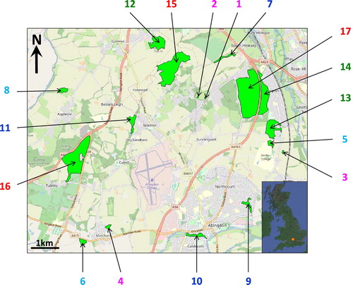
The study was carried out in Oxfordshire, UK, where the wooded landscape is highly fragmented and typical of that found in southern UK: within the county, woodland cover represents 7% of total land area and 93.4% of woodlands are under 10 ha (Smith & Gilbert 2002). In order to maximize comparability between encounter rates measured in different woodlands, the study used a single surveyor and a narrow spring survey window. An initial sample size of 20 woodlands was chosen, allowing each woodland to be surveyed on three separate days over two months. Google satellite images were used to identify woodlands within a 70 km² survey area and woodlands selected to give an even spread of sizes, with priority given to those with clearly defined boundaries. Permission was obtained to survey in all but three of the selected woodlands, leaving a final sample of 17 woodlands ranging in area from 0.2 to 120 ha. Figure 1 shows the woodland locations, with woodlands labelled 1–17 in order of increasing area. Surrounding external habitat varied from entirely urban (woodlands 9 and 10; Figure 1) to entirely agricultural (woodlands 3 and 8; Figure 1). None of the woodlands have shown significant area changes in the last 30 years, so time-dependent effects (due to the species richness response lagging behind any changes in woodland area) are assumed negligible within the sample.

Figure 1. Map showing locations of sample woodlands, where woodlands are labelled 1–17 in order of increasing woodland area. Label colour indicates the area bin each woodland belongs to: bin 1 woodlands (1, 2, 3 and 4; 0.20 ha < A < 2.23 ha) are magenta, bin 2 woodlands (5, 6 and 8; 3.63 ha < A < 5.23 ha) are cyan, bin 3 woodlands (7, 9, 10 and 11; 4.69 ha < A < 9.46 ha) are blue, bin 4 woodlands (12, 13 and 14; 21.70 ha < A < 36.18 ha) are green, and bin 5 woodlands (15, 16 and 17; 71.30 ha < A < 120.38 ha) are red. Inset shows location of study site within UK (orange point). Base maps from Open Street Map and Google Satellite.

Bird surveys

Dawn bird surveys were carried out between 1st April and 28th May 2016 to correspond with the peak song period. Since song activity decreases significantly as the morning progresses (Palmgren 1949), a strict survey window between sunrise and 2.5 h after sunrise was used in order to maximize comparability of encounter rates between surveys. Each woodland was surveyed three times, with stratified random scheduling used to determine woodland survey order. Where survey dates could not be randomly selected due to access constraints (two woodlands), care was taken to ensure one survey fell within each survey period. In the event of heavy rain or high winds, surveys were rescheduled to avoid adverse weather conditions depressing encounter rates.

Each survey consisted of an area search of the woodland, recording time of first encounter with each species and tallying all subsequent encounters. Species accumulation curves were constructed from the time of first encounter data, to check for comparable survey completeness across the entire area range, while the total number of encounters per species was divided by survey duration to obtain encounter rates per species. Precipitation (none/light rain/rain), wind conditions (still/light/breezy), cloud cover (none/patchy/full), temperature (UK Met Office prediction for Oxford) and type of encounter (visual/vocal/both) were recorded as quality-control data.

Standardized area searches were chosen since these offered the most comparable survey method across the 3 orders of magnitude area range, and they have been shown to yield more complete richness estimates than either transects or fixed effort searches (Watson 2004). Ideally, the route taken during the area search systematically covered the entire area of the woodland (including edge habitat), such that it intersected every potential territory, within the time limit of 2.5 h after sunrise. This was only possible for the 11 smallest woodlands (under 10 ha), given a constant walking speed of 1–2 km h⁻¹. For these woodlands, the survey ended when the entire area had been searched. At woodlands 12 and 15, access was only permitted to part of the woodland, reducing the surveyed area to 10.22 ha and 11.73 ha, respectively. In these woodlands, survey routes were more widely spaced in order to cover the entire survey area within the time limit. For woodlands 13, 14, 16 and 17, widely spaced routes were interlaced in order to cover the entire woodland area over the course of the three surveys, with each individual survey completed within the time limit. Routes were tracked using a Global Positioning System (GPS) unit to facilitate route variation and help achieve completeness of coverage. Where there were large areas of alternative habitat within the woodland (e.g. reedbed at woodlands 7, 9 and 11) routes were chosen which stayed as close to the woodland as possible. Where woodland edges were affected by road noise (in woodlands 6, 14, 16 and 17), these sections were avoided, as road noise can drown out vocalizations, reduce breeding bird density (Reijnen et al. 1995) and alter community composition (Francis et al. 2009), and care was taken to survey alternative sections of edge habitat.

Habitat surveys

The aim of the habitat survey was to quantify any differences between woodlands that may affect species richness and reduce comparability. Habitat surveys were conducted following the final bird survey of each woodland, as this sampled the maximum vegetation growth during the survey period.

Random sample locations were generated using QGIS software (version 2.10.1, QGIS Development Team 2015), with number of samples scaled with woodland area as $N\propto A^{1/3}$ (where A is the surveyable area of the woodland in the case of woodlands 12 and 15 where access is restricted). Five sample points were required in the smallest woodland, as a compromise between achieving sufficient data resolution (20%) without losing independence of sample locations, giving a sample size of 37 (maximum feasible with survey resources available) in the largest with the adopted scaling.

Sample points were located with a GPS unit, and presence/absence of habitat types in the immediate vicinity (within 4 m) recorded. Eleven habitat categories were adopted, based on those used by Hinsley et al. (1995) in their assessment of habitat factors influencing the presence of bird species in woodland fragments. The 11 categories were water (any pond, stream, river), reedbed (including sedgebed), open glade, thin ground layer, thick ground layer, short shrub layer (<1.5 m), tall shrub layer (>1.5 m), young scrub/young trees (<2 m), mature scrub (>2 m), mature coniferous trees, mature deciduous trees. The distinction between thin and thick ground layers was based on fractional cover as viewed from above combined with vegetation height and was subjective, however a single observer conducted all surveys, reducing observer variation. In general, where patches of bare ground were seen or the ground cover was short turf, the ground layer was classed as thin. Where herbaceous vegetation cover was roughly continuous (>90%) and between ankle and hip height, it was classed as thick ground cover.

Data analysis

Data from individual woodlands was binned before analysis to minimize the impact of habitat variations between woodlands. Woodlands were binned by increasing area into the following five bins: bin 1 contains woodlands 1, 2, 3 and 4 (0.20 ha < A < 2.23 ha); bin 2 contains woodlands 5, 6 and 8 (3.63 ha < A  < 5.23 ha); bin 3 contains woodlands 7, 9, 10 and 11 (4.69 ha < A < 9.46 ha); bin 4 contains woodlands 12, 13 and 14 (21.70 ha < A  < 36.18 ha); and bin 5 contains woodlands 15, 16 and 17 (71.30 ha < A < 120.38 ha). The woodlands in bin 3 all have a high perimeter:area ratio and contain a higher proportion of water and/or reedbed habitats, hence woodland 7 was assigned to this bin, despite having slightly smaller area than the largest woodland in bin 2.

The woodland bins were first tested for significant differences in habitat composition, which may affect the presence/absence of individual species and so influence community composition. Due to non-normality of the habitat data, Kruskal–Wallis tests were used to compare the median percentage of sample points containing each habitat type across the five area bins and the total number of habitat types present across the five area bins.

The woodland bins were then tested for significant differences in total species richness using a one-way analysis of variance (ANOVA; when comparing bins 1, 2, 4 and 5, where data was normally distributed within the bins) and the Kruskal–Wallis test (when additionally comparing bin 3, which contained non-normal data). The one-way ANOVA and all Kruskal–Wallis tests were carried out using QED statistics (Henderson & Seaby 2007).

In order to investigate changes in community composition, we used the habitat groups assigned to each species by DEFRA (2017), which are used to calculate UK-wide population trends, to divide species into three guilds: non-woodland species are those that do not depend on woodland, woodland generalists are woodland species that have adapted to live in other habitats, and woodland specialists are species that are strongly dependent on woodland. For each individual woodland, we calculated (1) the mean number of species from each guild recorded across its three surveys and (2) the mean fraction of the total encounter rate that is due to each guild across its three surveys. For each woodland bin, we then calculated (1) the mean number of species from each guild across all the woodlands in that bin and (2) the mean fraction of the total encounter rate that is due to each guild across all the woodlands in that bin. Mean fraction of the total encounter rate is a measure of the relative abundance of each guild across the woodland bins (assuming detectability remains constant). We assessed the dependence of the mean number of species ($\overline{N}$) from each guild (D) on the mean area ($\overline{A}$) of the woodland bin by fitting the linear model: lm($\overline{N}$∼log₁₀($\overline{A}$)*D, $\mathrm{w}\mathrm{e}\mathrm{i}\mathrm{g}\mathrm{h}\mathrm{t}\mathrm{s}=1/{\epsilon }_{\overline{N}}$), where ${\epsilon }_{\overline{N}}$ is the standard error on $\overline{N}$. We assessed the dependence of the mean fractional contribution to the total encounter rate ($\overline{F}$) of each guild on the mean area of the woodland bin by fitting the linear model: lm($\overline{F}$∼log₁₀($\overline{A}$)*D, weights = 1/${\epsilon }_{\overline{F}}$), where ${\epsilon }_{\overline{F}}$ is the standard error on $\overline{F}$. In both cases, the weights allow the models more freedom where the uncertainty on the mean is large. The linear models were fitted using R version 3.4.3 (R Core Team 2017).

Results

Habitat surveys

Figure 2 shows the median percentage of sample locations recording each habitat type for each area bin (note that habitat types are not mutually exclusive and more than one may be recorded at a given sample location). Nine out of the 11 habitat types were present in all five area bins. The remaining habitats were reedbed (recorded only in bin 3) and mature scrub (recorded in bins 2 and 3). The mature scrub fraction of bin 2 was due to a single sample location in woodland 6 and so deemed negligible. Of the nine habitats which were present in all five bins, water and tall shrub layer were the only two where a significant difference was found in the median percentage of sample locations across the five bins (Kruskal–Wallis test; K = 11.2, df = 4, P = 0.025 for water; K = 9.98, df = 4, P = 0.041 for tall shrub layer). When bin 3 was excluded from the analysis, the difference between the medians of the remaining bins was not significant (Kruskal–Wallis test; K = 3.95, df = 3, P = 0.267 for water; K = 4.26, df = 3, P = 0.235 for tall shrub layer).

Figure 2. Binned habitat data. Bar heights show median percentage of sample locations recording each habitat type, for each of the five woodland area bins. Within each habitat category, area bins are plotted so that woodland area increases from left to right (magenta to red), with the colours corresponding to those used in Figure 1. Vertical error bars show positions of the upper and lower quartiles within each bin.

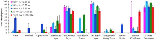
Bin 3 therefore showed significantly different habitat composition compared to the other four bins: a higher fraction of sample locations recorded water, a lower fraction recorded tall shrub layer and it included two additional habitat types (reedbed and mature scrub). The four remaining bins were consistent with the same habitat composition, with no significant difference between median percentage of sample locations recording each habitat type.

Total number of habitats can affect species richness and the larger a wood is, the more potential for it to contain a greater variety of habitats. We found there was no significant difference in the median number of habitat types across the five area bins, regardless of whether woodland 4 (which had a larger number of habitats than other woodlands in the smallest area bin) was included or not (Kruskal–Wallis test; K = 6.35, df = 4, P = 0.175 including woodland 4; K = 7.63, df = 4, P = 0.106 excluding woodland 4).

Bird surveys

In total, 12 715 encounters were recorded with 53 different species. Table 1 lists the number of woodlands each species was recorded in and the guild the species belongs to (non-woodland, 29 species; woodland generalist, 11 species; woodland specialist, 13 species). Species accumulation curves from all surveys showed flattening at late times, suggesting comparable completeness was achieved by the end of each survey across all woodlands.

Table 1. List of species encountered, sorted by the number of woods in which each was recorded.

Common Name	Scientific Name	Guild	No. of Woods
Woodpigeon	Columba palumbus	N	17
Wren	Troglodytes troglodytes	G	17
Robin	Erithacus rubecula	G	17
Blackbird	Turdus merula	G	17
Blue Tit	Parus caeruleus	G	17
Great Tit	Parus major	G	17
Carrion Crow	Corvus corone	N	17
Song Thrush**	Turdus philomelos	G	16
Chaffinch	Fringilla coelebs	G	16
Dunnock*	Prunella modularis	G	15
Blackcap	Sylvia atricapilla	S	15
Chiffchaff	Phylloscopus collybita	S	15
Goldcrest	Regulus regulus	S	15
Long-tailed Tit	Aegithalos caudatus	G	15
Coal Tit	Parus ater	S	15
Nuthatch	Sitta europaea	S	15
Pheasant	Phasianus colchicus	N	14
Great Spotted Woodpecker	Dendrocopos major	S	14
Magpie	Pica pica	N	14
Jackdaw	Corvus monedula	N	14
Green Woodpecker	Picus viridis	S	13
Goldfinch	Carduelis carduelis	N	13
Jay	Garrulus glandarius	S	12
Treecreeper	Certhia familiaris	S	11
Willow Warbler*	Phylloscopus trochilus	S	10
Common Buzzard	Buteo buteo	N	9
Greenfinch	Carduelis chloris	N	9
Stock Dove*	Columba oenas	N	8
Collared Dove	Streptopelia decaocto	N	8
Bullfinch*	Pyrrhula pyrrhula	G	7
Red Kite	Milvus milvus	N	6
Mallard*	Anas platyrhynchos	N	5
Sparrowhawk	Accipiter nisus	S	5
Moorhen	Gallinula chloropus	N	5
Mistle Thrush**	Turdus viscivorus	N	5
Whitethroat	Sylvia communis	N	5
Reed Warbler	Acrocephalus scirpaceus	N	4
Marsh Tit**	Parus palustris	S	4
Tawny Owl*	Strix aluco	G	3
Yellowhammer**	Emberiza citrinella	N	3
Grey Heron	Ardea cinerea	N	2
Wood Warbler**	Phylloscopus sibilatrix	S	2
Rook	Corvus frugilegus	N	2
Reed Bunting*	Emberiza schoeniclus	N	2
Little Egret	Egretta garzetta	N	1
Mute Swan*	Cygnus olor	N	1
Canada Goose	Branta canadensis	N	1
Tufted Duck	Aythya fuligula	N	1
Little Owl	Athene noctua	N	1
Kingfisher*	Alcedo atthis	N	1
Starling**	Sturnus vulgaris	N	1
House Sparrow**	Passer domesticus	N	1
Linnet**	Carduelis cannabina	N	1

Species guilds follow those given in DEFRA (2017): N = non-woodland species, G = woodland generalists, S = woodland specialists. Species of conservation concern in the UK are indicated by asterisks (* = amber list, ** = red list) according to Eaton et al. (2015), where the amber list includes species of moderate conservation concern and the red list includes those species of highest conservation concern.

Total species richness

Total species richness increased with area up to approximately 3.6 ha, after which the correlation saturated at roughly constant total richness despite further increases in area (Figure 3).

Figure 3. Total number of species as a function of woodland area. Grey crosses show results of individual surveys. Coloured circles show the mean of the three surveys for each woodland, where woodlands within the same area bin share the same colour, as in Figure 1. Error bars show standard error on the mean.

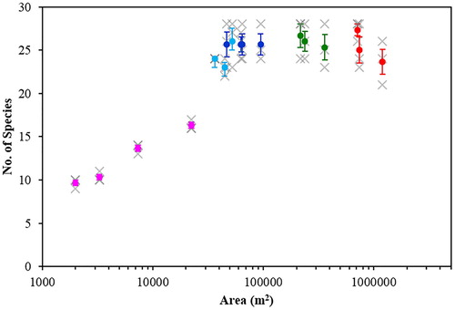
Excluding bin 3 (due to its different habitat composition), there was a highly significant difference between the mean total species richness of the other four woodland area bins (one-way ANOVA, F_3,9 = 32.927, P < 0.001). However, if the smallest area bin was also excluded, there was no significant difference between the three remaining bin means (one-way ANOVA, F_2,6 = 1.018, P = 0.416). From Figure 3, it is clear that the woodlands in bin 3 showed comparable total species richness to woodlands in the other three saturated bins, despite habitat differences, and a Kruskal–Wallis test (due to non-normality of the bin 3 data) confirmed no significant difference in median total species richness between bin 3 and the other saturated bins (K = 2.07, df = 3, P = 0.557). The woodlands larger than 3.6 ha were therefore all consistent with the same total species richness (mean ± se = 25.4 ± 0.6 species), while the bin containing woodlands with area less than 3.6 ha had significantly lower total species richness.

The four smallest woodlands showed an increase in total species richness with area. Simple linear regression on these four data points (weighting the contribution of each point to the fit by the inverse of its standard error), plus a fifth point which had mean total species richness calculated from the 13 remaining woodlands (mean ± se = 25.4 ± 0.6) and area equal to the minimum area of the first saturated bin, gave ${\log }_{10}N=\left(0.32\pm 0.06\right){\log }_{10}A-\left(0.1\pm 0.2\right)$ where A is measured in m², for A < 3.63 ha. The regression was statistically significant (F = 32.7, df = (1,3), P = 0.011) and the adjusted coefficient of determination R²= 0.888, implying almost 90% of the variation in total species richness was accounted for by variation in woodland area in this case.

Community composition

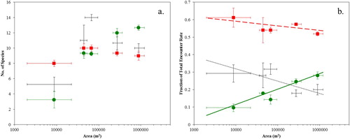
Figure 4(a) shows the individual contributions of non-woodland species, woodland generalists and woodland specialists to the total species richness in each woodland area bin. The large number of non-woodland species recorded in area bin 3 (4.69 ha < A < 9.46 ha) was a result of the significantly different habitat composition of these wet woodlands. In the smallest area bin, there were more woodland generalist species recorded than woodland specialists, while in the largest area bin, there were more woodland specialist species recorded than woodland generalists.

Although the total species richness was constant for woodlands larger than 3.6 ha (Figure 3), Figure 4(a) shows that the relative contributions of the three guilds were changing, with the contribution of woodland specialists to the total species richness increasing with woodland area, while the contribution of woodland generalists and non-woodland species moderately decreased (excluding bin 3). Concentrating on the bins where total species richness has saturated (i.e. excluding bin 1), and excluding bin 3 (which had significantly different habitat composition), we fitted the linear model to the remaining three bins (bins 2, 4 and 5) and obtained the results shown in Table 2. There was a significant interaction between woodland area and guild (F = 27.3, df = 2, P = 0.012); although the area dependences for non-woodland species and woodland generalists were not significantly different from zero, due to the small sample size and weakness of the trends, the positive area dependence for woodland specialists was significant (Table 2). This confirmed the contribution of woodland specialists to the total species richness did continue to increase with woodland area after saturation of total species richness.

Table 2. Results from regressing the mean number of species recorded from each guild in a woodland bin ($\overline{N}\left(N,G,S\right)$) against the mean woodland area of the bin ($\overline{A}$) using a linear model.

Coefficient	Estimate	Standard error	t value	P(>|t|)
αN	15	3	5.08	0.015	*
αG	14	2	7.02	0.006	**
αS	−2	2	−1.18	0.323
βN	−0.8	0.5	−1.58	0.212
βG	−0.8	0.4	−2.16	0.119
βS	2.5	0.3	7.49	0.005	**

Linear model equation: $\overline{N}=\left(\begin{array}{c}{\alpha }_N\\ {\alpha }_G\\ {\alpha }_S\end{array}\right)+{\log }_{10}\overline{A}\left(\begin{array}{c}{\text{β}}_N\\ {\text{β}}_G\\ {\text{β}}_S\end{array}\right)$, where $\overline{A}$ is measured in m² and the subscripts N, G and S refer to the coefficients relating to non-woodland species, woodland generalists and woodland specialists, respectively. Model was fitted using data from bin 2, bin 4 and bin 5 woodlands, where data points were weighted by 1/${\epsilon }_{\overline{N}}$, where ${\epsilon }_{\overline{N}}$ is the standard error on $\overline{N}$. Coefficients which are statistically significantly different from zero are marked with asterisks (*P < 0.05, **P < 0.01).

Figure 4(b) shows the mean fraction of the total encounter rate that is due to non-woodland species, woodland generalists and woodland specialists in each area bin. In all area bins, the total encounter rate was dominated by woodland generalists. The fractional contribution of woodland specialists clearly increased with woodland area, while the fractional contributions of woodland generalists and non-woodland species correspondingly decreased. For the smallest area bins, the fractional contribution of non-woodland species exceeded that of woodland specialists by a factor of 3, while for the largest area bins, the fractional contribution of woodland specialists exceeded non-woodland species.

Fitting the linear model using fractional encounter rate data from all bins gave the results shown in Table 3. Again, there was a significant interaction between woodland area and guild (F = 11.8, df = 2, P = 0.003); the fractional contribution of non-woodland species to the total encounter rate showed a significant negative trend with woodland area, while the contribution of woodland generalists showed no significant trend with area, and the fractional contribution of woodland specialists to the total encounter rate showed a significant positive trend with woodland area (Table 3).

Table 3. Results from regressing the mean fractional contribution of each guild to the total encounter rate of a woodland bin ($\overline{F}\left(N,G,S\right)$) against the mean woodland area of the bin ($\overline{A}$) using a linear model.

Coefficient	Estimate	Standard Error	t value	P(>|t|)
αN	0.6	0.2	3.84	0.004	**
αG	0.7	0.1	5.21	0.001	**
αS	−0.24	0.10	−2.40	0.040	*
βN	−0.07	0.03	−2.33	0.045	*
βG	−0.03	0.02	−1.05	0.321
βS	0.09	0.02	4.32	0.002	**

Linear model equation: $\overline{F}=\left(\begin{array}{c}{\alpha }_N\\ {\alpha }_G\\ {\alpha }_S\end{array}\right)+{\log }_{10}\overline{A}\left(\begin{array}{c}{\text{β}}_N\\ {\text{β}}_G\\ {\text{β}}_S\end{array}\right)$, where $\overline{A}$ is measured in m² and the subscripts N, G and S refer to the coefficients relating to non-woodland species, woodland generalists and woodland specialists, respectively. Model was fitted using data from all five woodland bins, where data points were weighted by 1/${\epsilon }_{\overline{F}}$, where ${\epsilon }_{\overline{F}}$ is the standard error on $\overline{F}$. Coefficients which are statistically significantly different from zero are marked with asterisks (*P < 0.05, **P < 0.01).

The data from bin 3 were in better agreement with the trends from other bins when comparing fractional encounter rate data than comparing guild species numbers (Figure 4). This is because the additional species inflating the non-woodland species numbers were due to a small number of individuals making use of the additional habitat types within bin 3 woodlands and so had a small effect on the total encounter rate. Refitting the linear model for mean fractional contribution to the total encounter rate, excluding bin 3, did not substantially alter the conclusions: although the significance of the negative area dependence for non-woodland species became marginal due to the reduced sample size, the positive area dependence for woodland specialists remained significant.

Figure 4. (a) Mean number of species per guild in each woodland area bin, and (b) mean fraction of the total encounter rate that is contributed by each guild in each woodland area bin, where the guilds are: non-woodland species (black crosses), woodland generalists (red squares) and woodland specialists (green circles). Vertical error bars show standard error on the mean. Horizontal error bars show the areas of the largest and smallest woodlands in each area bin. Black dotted line, red dashed line and green solid line in (b) show linear model fit from Table 3 for non-woodland species, woodland generalists and woodland specialists, respectively.

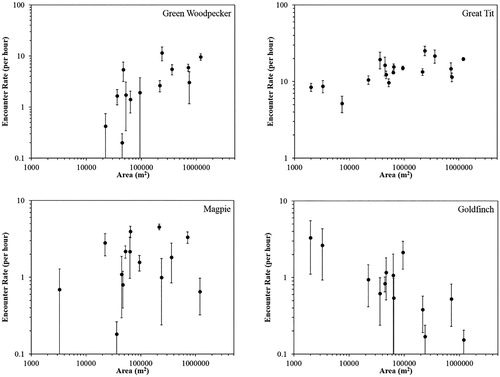
Figure 5 shows encounter rate as a function of woodland area for a selection of species. These illustrate some of the species–level effects contributing to the community composition trends shown in Figure 4. Top left panel of Figure 5 shows a woodland specialist (Green Woodpecker Picus viridis), which was absent from the smallest woodlands. Top right panel shows a woodland generalist (Great Tit Parus major), which was present in the smallest woodlands but showed higher encounter rates in larger woodlands, suggesting these may offer better habitat conditions (as also found by Bueno-Enciso et al. 2016). Bottom left panel shows an area-insensitive non-woodland species (Magpie Pica pica), which occurred sporadically throughout the area range. Bottom right panel shows an interior-averse non-woodland species (Goldfinch Carduelis carduelis), which showed higher encounter rates in smaller woodlands.

Figure 5. Encounter rate as a function of woodland area for a woodland specialist (Green Woodpecker Picus viridis), a woodland generalist (Great Tit Parus major), an area-insensitive non-woodland species (Magpie Pica pica) and an interior-averse non-woodland species (Goldfinch Carduelis carduelis). Each black point shows the mean encounter rate across the three surveys in a given woodland. Error bars show standard error on the mean.

Non-woodland species

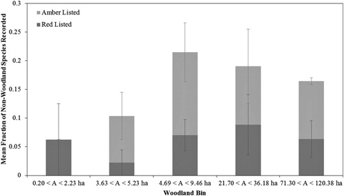
Figure 4 shows that many non-woodland species were making use of the sample woodlands. Although woodland reserves are naturally aimed at supporting woodland birds, many of these non-woodland species are also of conservation concern (Table 1). Figure 6 shows the mean fraction of non-woodland species recorded in each woodland bin that are considered to be of conservation concern in the UK according to Eaton et al. (2015). The bin 3 woodlands contained the largest fraction, with the fraction of non-woodland species of conservation concern decreasing sharply for smaller woodlands and less steeply for larger woodlands.

Figure 6. Mean fraction of non-woodland species recorded that are red listed and amber listed in each woodland bin, according to the UK conservation status assigned to each species by Eaton et al. (2015), where the amber list includes species of moderate conservation concern and the red list includes those species of highest conservation concern.

Discussion

Our study showed that woodlands smaller than 3.6 ha had significantly lower total species richness and showed a significant positive relationship between total species richness and woodland area. Woodlands larger than 3.6 ha were consistent with a mean (±se) total richness of 25.4 ± 0.6 species. If we rely solely on the total species richness-area relation, we therefore conclude that woodlands larger than 3.6 ha provide the most valuable woodland habitat, since these all show the maximum total species richness. Woodlands smaller than this threshold are primarily valuable as habitat stepping stones, while all woodlands larger than this threshold are indistinguishable, all appearing to provide sufficient conditions for this maximum number of species. We can make only one recommendation: that new woodland reserves (whether planted or created from existing woodland) should ideally be larger than this 3.6 ha threshold in order to maximize total avian species richness.

However, analysing the community composition of these woodlands revealed significant changes in guild species numbers and encounter rates, beneath the trend in total species richness (Figure 4). Woodlands above the 3.6 ha threshold clearly did not all provide the same level of benefit to woodland specialists, woodland generalists and non-woodland species. For instance, in the smaller woodlands, non-woodland species were more likely to be encountered than woodland specialists, and vice versa in the largest woodlands (Figure 4(b)). Furthermore, the 3.6 ha threshold itself becomes less meaningful when examining species numbers per guild (Figure 4(a)).

The contribution of woodland specialists to the total species richness continued to increase with woodland area (Figure 4(a)), despite the saturation of total species richness at 3.6 ha. Our results agree with the findings of Matthews et al. (2014), who combined data from multiple studies to show that richness of woodland specialists can exhibit a stronger dependence on woodland area, which can be masked when simply considering total species richness. The fractional contribution of woodland specialists to the total encounter rate significantly increased with woodland area across the entire area range (Figure 4(b)), implying woodland specialists represent a larger fraction of the avian community in larger woodlands (assuming constant detectability with area), and Figure 5 suggests this may not be solely due to larger woodlands containing more woodland specialist species, but also due to individual woodland species showing higher encounter rates (i.e. higher abundance) in larger woodlands. This suggests bigger woodlands are better for woodland specialists. However, we found even the largest woodlands did not contain all woodland specialists recorded during the study, as also noted by Robbins et al. (1989). Internal habitat is important and can be a limiting factor for species with specific habitat requirements (Hewson et al. 2011). This suggests (1) new woodland reserves aimed specifically at providing habitat for woodland specialists should ideally be much larger than the 3.6 ha threshold implied by our examination of total species richness, and (2) large woodlands (over 25 ha) should focus management efforts on providing the specific internal habitats required by woodland specialists.

The 3.6 ha threshold is also not particularly meaningful for non-woodland species, which showed a maximum in species numbers in the medium-sized bin 3 woodlands, with lower species numbers occurring in both smaller and larger woodlands (Figure 4(a)). The fraction of non-woodland species that are of conservation concern also peaked in these medium-sized bin 3 woodlands (Figure 6). These bin 3 woodlands showed significantly different habitat composition and internal habitat variety (e.g. presence of clearings and ponds) can increase the attractiveness of a woodland to non-woodland species, e.g. Linnets Carduelis cannabina using gorse within agricultural woodland 12, House Sparrows Passer domesticus using scrub within urban woodland 9 and wetland birds in bin 3 woodlands. Bellamy et al. (1996) found that the number of edge-species correlates with perimeter length, so the high perimeter:area ratios of some medium-sized woodlands may be a contributing factor (Figure 1), along with the concentration of watercourse/wetland perimeter woodlands in bin 3. However, an additional factor may be that such medium-sized woodlands are typical of the type adopted by conservation organizations and as such may receive more regular management designed to promote internal habitat variety. This suggests that, in addition to providing habitat for woodland specialists and generalists, medium-sized woodlands can also provide important benefits for non-woodland species in the surrounding landscape which may also be of conservation concern. The fractional contribution of non-woodland species to the total encounter rate significantly decreased with increasing woodland area (Figure 4(b)) so, crucially, these woodlands are large enough to contain internal habitat variety but not so large that potentially interior-averse non-woodland species are discouraged from entering them. This suggests that medium-sized woodlands (approximately between 4 and 25 ha) should focus management efforts on maximizing internal habitat variety, in order to benefit both woodland species and non-woodland species of conservation concern in the surrounding landscape.

Out of the three guilds, woodland generalists dominated the total encounter rate across the area range (Figure 4(b)) and also showed the smallest change in species numbers across the area range (a mean of 8 species in the smallest area bin versus 9–10 species for bins above the 3.6 ha threshold; Figure 4(a)). This small change in species numbers with area is likely a reflection of these species’ ability to make use of additional habitats beyond the wooded environment and/or a greater willingness to cross habitat gaps and make use of multiple smaller woodlands (Tjernberg et al. 1993). This suggests that woodlands smaller than the 3.6 ha threshold still provide important resources for woodland birds and that landowners of small woodlands (less than 4 ha) should focus efforts on improving their connectivity via hedgerows and/or planting other small woodlands nearby, in order to maximize habitat for woodland generalists and facilitate movement of woodland specialists.

Our study has shown that examining species numbers per guild, and including information on the relative abundance of these guilds, both highlights the limitations of the total richness approach and allows us to significantly improve on its simple minimum area recommendations. Instead of focusing on binary area cut-offs, the community composition approach allows us to recognize and quantify the value of different sized woodlands to different groups of birds. Crucially, it allows us to identify guild-specific recommendations for optimizing woodland habitat across the entire woodland area range, enabling targeted recommendations that reflect the interdependence of woodland area and avian community composition.

Assumptions and caveats

We have equated changes in fractional encounter rate to changes in relative abundance by assuming that the detectability of individual species does not vary between woodlands and, crucially, that it does not vary with area. Vegetation density can reduce visibility, however there were no significant differences in habitat composition between the area bins (excluding bin 3) and on average 85% of encounters involved vocal detections, which are less affected by habitat variation. Species may sing less in very small woodlands, due to lack of neighbouring individuals reducing song rate (McShea & Rappole 1997), however care was taken to compensate for this by searching for visual detections, with visual-only detections constituting on average 40% of detections in the three smallest woodlands, compared to 15% across the entire sample.

Proximity to other woodlands can influence presence/absence of some woodland species (Opdam et al. 1984); where woodlands are close together, species not averse to gap crossing may make use of multiple small woodlands (Tjernberg et al. 1993), while dispersion between woodlands may be a problem when woodlands are far apart (Matthysen & Currie 1996). Increased isolation can therefore reduce species richness (Chang et al. 2017). All study woodlands were less than 0.7 km from another woodland. Many passerines typically disperse less than ten territories from hatching sites (Greenwood & Harvey 1982), with female Great Tits dispersing on average 0.879 km (Greenwood et al. 1979). Note that dispersal distances measured by Greenwood et al. (1979) in Wytham Woods (southern England), where nest boxes are provided, may be more conservative than those in other areas; Paradis et al. (1998) found typical dispersal distances of a few kilometres for woodland birds, while ringing data from Redcar and Cleveland (northern England) has shown Great Tit dispersal distances of 6 km for multiple individuals, although these are a minority (T. Dewdney, pers. comm.). This implies dispersion may be less restricted within our sample, and spatial independence affected in some cases. Therefore, in regions with poorer connectivity than the study area, woodland specialists in particular may show a stronger decline in species numbers and encounter rates with decreasing area, causing a corresponding increase in the minimum area derived from analysing total species numbers.

All surveys were conducted in established woodlands. Newly created woodlands show a time delay between creation and subsequent colonization, with woodland specialists showing significantly longer time lags than generalists (Whytock et al. 2018). This time lag will be affected by the management regime within the new woodland and its proximity to established woodland specialist populations. This implies new small woodlands (aimed at maximizing habitat for woodland generalists) may achieve their maximum species numbers and steady-state community composition faster than new large woodlands (aimed at conserving woodland specialists), which may require over 50 years to achieve the required stand structure and subsequent colonization by woodland specialists (Whytock et al. 2018).

Our study area represents habitat typical of the highly modified landscape of southern UK. Similar scale studies in other regions are needed to shed light on the extent to which our management recommendations and area definitions for small, medium-sized and large woodlands should be adjusted in landscapes with better/poorer woodland connectivity and with more/less well established woodland bird populations.

Acknowledgements

We would like to thank two anonymous reviewers for their helpful comments. EG acknowledges very helpful conversations with P. Bellamy, R. Whytock, K. Watts and T. Dewdney during the course of this research. This project would not have been possible without the woodland owners, farmers and organizations who kindly allowed access to their land and those who assisted in the process, including Abingdon Green Gym, Abingdon Town Council, All Souls College, Berkshire, Buckinghamshire and Oxfordshire Wildlife Trust, Cumnor Conservation Group, Cumnor Parish Council, Earth Trust, Marcham Society, Oxford City Council, Oxford Conservation Volunteers, Oxford Preservation Trust, Radley College, Radley Parish Council, St. John's College, Vale of the White Horse District Council, Youlbury Scout Activity Centre, G. Broughton, P. Dockar-Drysdale, N. Frearson, D. Gow, C. Little and M. Wiseman.

References

- Bellamy, P.E., Hinsley, S.A. & Newton, I. 1996. Factors influencing bird species numbers in small woods in south-east England. J. Appl. Ecol. 33: 249–262. doi: 10.2307/2404747
- Bennett, J.M., Clarke, R.H., Thomson, J.R. & Mac Nally, R. 2015. Fragmentation, vegetation change and irruptive competitors affect recruitment of woodland birds. Ecography 38: 163–171. doi: 10.1111/ecog.00936
- Biz, M., Cornelius, C. & Metzger, J.P.W. 2017. Matrix type affects movement behavior of a Neotropical understory forest bird. Perspect. Ecol. Conserv. 15: 10–17.
- Brudvig, L.A., Leroux, S.J., Albert, C.H., Bruna, E.M., Davies, K.F., Ewers, R.M., Levey, D.J., Pardini, R. & Resasco, J. 2017. Evaluating conceptual models of landscape change. Ecography 40: 74–84. doi: 10.1111/ecog.02543
- Bueno-Enciso, J., Ferrer, E.S., Barrientos, R., Serrano-Davies, E. & Sanz, J.J. 2016. Habitat fragmentation influences nestling growth in Mediterranean blue and great tits. Acta Oecol. 70: 129–137. doi: 10.1016/j.actao.2015.12.008
- Carrara, E., Arroyo-Rodríguez, V., Vega-Rivera, J.H., Schondube, J.E., de Freitas, S.M. & Fahrig, L. 2015. Impact of landscape composition and configuration on forest specialist and generalist bird species in the fragmented Lacandona rainforest, Mexico. Biol. Conserv. 184: 117–126. doi: 10.1016/j.biocon.2015.01.014
- Chang, C.R., Chien, H.F., Shiu, H.J., Ko, C.J. & Lee, P.F. 2017. Multiscale heterogeneity within and beyond Taipei city greenspaces and their relationship with avian biodiversity. Landsc. Urban Plann. 157: 138–150. doi: 10.1016/j.landurbplan.2016.05.028
- DEFRA. 2017. Wild Bird Populations in the UK, 1970–2016: Annual Statistical Release. DEFRA. https://www.gov.uk/government/statistics/wild-bird-populations-in-the-uk
- Desrochers, A. & Hannon, S.J. 1997. Gap crossing decisions by forest songbirds during the post-fledging period. Conserv. Biol. 11: 1204–1210. doi: 10.1046/j.1523-1739.1997.96187.x
- Eaton, M.A., Aebischer, N.J., Brown, A., Hearn, R.D., Lock, L., Musgrove, A.J., Noble, D.G., Stroud, D.A. & Gregory, R.D. 2015. Birds of conservation concern 4: the population status of birds in the UK, Channel Islands and Isle of Man. Br. Birds 108: 708–746.
- Francis, C.D., Ortega, C.P. & Cruz, A. 2009. Noise pollution changes avian communities and species interactions. Curr. Biol. 19: 1415–1419. doi: 10.1016/j.cub.2009.06.052
- Freeman, M.T., Olivier, P.I. & van Aarde, R.J. 2018. Matrix transformation alters species-area relationships in fragmented coastal forests. Landsc. Ecol. 33: 307–322. doi: 10.1007/s10980-017-0604-x
- Galli, A.E., Leck, C.F. & Forman, R.T.T. 1976. Avian distribution patterns in forest islands of different sizes in central New Jersey. Auk 93: 356–364.
- Greenwood, P.J. & Harvey, P.H. 1982. The natal and breeding dispersal of birds. Annu. Rev. Ecol. Syst. 13: 1–21. doi: 10.1146/annurev.es.13.110182.000245
- Greenwood, P.J., Harvey, P.H. & Perrins, C.M. 1979. The role of dispersal in the great tit (Parus major): the causes, consequences and heritability of natal dispersal. J. Anim. Ecol. 48: 123–142. doi: 10.2307/4105
- Haas, C.A. 1995. Dispersal and use of corridors by birds in wooded patches on an agricultural landscape. Conserv. Biol. 9: 845–854. doi: 10.1046/j.1523-1739.1995.09040845.x
- Haila, Y. 2002. A conceptual genealogy of fragmentation research: from island biogeography to landscape ecology. Ecol. Appl. 12: 321–334.
- Henderson, P.A. & Seaby R. H. M. 2007. QED Statistics 1.1. Pisces Conservation Ltd, Lymington.
- Hewson, C.M., Austin, G.E., Gough, S.J. & Fuller, R.J. 2011. Species-specific responses of woodland birds to stand-level habitat characteristics: the dual importance of forest structure and floristics. For. Ecol. Manag. 261: 1224–1240. doi: 10.1016/j.foreco.2011.01.001
- Hill, J.K., Gray, M.A., Khen, C.V., Benedick, S., Tawatao, N. & Hamer, K.C. 2011. Ecological impacts of tropical forest fragmentation: how consistent are patterns in species richness and nestedness? Philos. Trans. R. Soc. B 366: 3265–3276. doi: 10.1098/rstb.2011.0050
- Hinsley, S.A., Bellamy, P.E., Newton, I. & Sparks, T.H. 1995. Habitat and landscape factors influencing the presence of individual breeding bird species in woodland fragments. J. Avian Biol. 26: 94–104. doi: 10.2307/3677057
- Hinsley, S.A., Bellamy, P.E., Newton, I. & Sparks, T.H. 1996. Influences of population size and woodland area on bird species distributions in small woods. Oecologia 105: 100–106. doi: 10.1007/BF00328797
- Le Roux, D.S., Ikin, K., Lindenmayer, D.B., Manning, A.D. & Gibbons, P. 2015. Single large or several small? Applying biogeographic principles to tree-level conservation and biodiversity offsets. Biol. Conserv. 191: 558–566. doi: 10.1016/j.biocon.2015.08.011
- Macnally, R. & Bennett, A.F. 1997. Species-specific predictions of the impact of habitat fragmentation: local extinction of birds in the box-ironbark forests of central Victoria, Australia. Biol. Conserv. 82: 147–155. doi: 10.1016/S0006-3207(97)00028-1
- MacArthur, R.H. & Wilson, E.O. 1967. The Theory of Island Biogeography, Monographs in Population Biol., Princeton Univ. Press, Princeton.
- Margules, C., Higgs, A.J. & Rafe, R.W. 1982. Modern biogeographic theory: are there any lessons for nature reserve design? Biol. Conserv. 24: 115–128. doi: 10.1016/0006-3207(82)90063-5
- Matthews, T.J., Cottee-Jones, H.E. & Whittaker, R.J. 2014. Habitat fragmentation and the species–area relationship: a focus on total species richness obscures the impact of habitat loss on habitat specialists. Divers. Distrib. 20: 1136–1146. doi: 10.1111/ddi.12227
- Matthysen, E. & Currie, D. 1996. Habitat fragmentation reduces disperser success in juvenile nuthatches Sitta europaea: evidence from patterns of territory establishment. Ecography 19: 67–72. doi: 10.1111/j.1600-0587.1996.tb00156.x
- McShea, W.J. & Rappole, J.H. 1997. Variable song rates in three species of passerines and implications for estimating bird populations. J. Field Ornithol. 68: 367–375.
- Opdam, P., van Dorp, D. & Ter Braak, D.J.F. 1984. The effect of isolation on the number of woodland birds in small woods in the Netherlands. J. Biogeogr. 11: 473–478. doi: 10.2307/2844793
- Palik, B.J. & Murphy, P.G. 1990. Disturbance versus edge effects in sugar-maple/beech forest fragments. For. Ecol. Manag. 32: 187–202. doi: 10.1016/0378-1127(90)90170-G
- Palmgren P. 1949. On the diurnal rhythm of activity and rest in birds. Ibis 91: 561–576. doi: 10.1111/j.1474-919X.1949.tb02311.x
- Paradis, E., Baillie, S.R., Sutherland, W.J. & Gregory, R.D. 1998. Patterns of natal and breeding dispersal in birds. J. Anim. Ecol. 67: 518–536. doi: 10.1046/j.1365-2656.1998.00215.x
- QGIS Development Team. 2015. QGIS Geographic Information System. Open Source Geospatial Foundation Project. https://qgis.org
- R Core Team. 2017. R: A language and environment for statistical computing. R Foundation for Statistical Computing, Vienna. https://www.R-project.org/
- Reijnen, R., Foppen, R., Braak, C.T. & Thissen, J. 1995. The effects of car traffic on breeding bird populations in woodland. iii. reduction of density in relation to the proximity of main roads. J. Appl. Ecol. 32: 187–202. doi: 10.2307/2404428
- Robbins, C.S., Dawson, D.K. & Dowell, B.A. 1989. Habitat area requirements of breeding forest birds of the middle Atlantic states. Wildl. Monogr. 103: 3–34.
- Smith, S. & Gilbert, J. 2002. National Inventory of Woodland and Trees: County Report for Oxfordshire. Forestry Commission, Edinburgh.
- Smith, S. & Gilbert, J. 2003. National Inventory of Woodland and Trees: Great Britain. Forestry Commission, Edinburgh.
- Spellerberg, I.F. & Sawyer, J.W.D. 1999. An Introduction to Applied Biogeography, 170. Cambridge University Press, Cambridge.
- Tew, N. & Hesselberg, T. 2017. The effect of wind exposure on the web characteristics of a tetragnathid orb spider. J. Insect Behav. 30: 273–286. doi: 10.1007/s10905-017-9618-0
- Tjernberg, M., Johnsson, K. & Nilsson, S.G. 1993. Density variation and breeding success of the black woodpecker Dryocopus-martius in relation to forest fragmentation. Ornis Fenn. 70: 155–162.
- Valentine, E.C., Apol, C.A. & Proppe, D. S. 2018. Predation on artificial avian nests is higher in forests bordering small anthropogenic openings. Ibis 161: 662–673. doi: 10.1111/ibi.12662
- Watson, D.M. 2004. Comparative evaluation of new approaches to survey birds. Wildl. Res. 31: 1–11. doi: 10.1071/WR03022
- Whitcomb, B.L., Whitcomb, R.F. & Bystrak, D. 1977. Island biogeography and ‘habitat islands’ of eastern forest. iii. Long-term turnover and effects of selective logging on the avifauna of forest fragments. American Birds 31: 17–23.
- Whytock, R.C., Fuentes-Montemayor, E., Watts, K., Barbosa De Andrade, P., Whytock, R.T., French, P., Macgregor, N.A. & Park, K.J. 2018. Bird-community responses to habitat creation in a long-term, large-scale natural experiment. Conserv. Biol. 32: 345–354. doi: 10.1111/cobi.12983
- Wilkin, T. A., Garant, D., Gosler, A. & Sheldon, B. C. 2006. Density effects on life-history traits in a wild population of the great tit Parus major: analyses of long-term data with GIS techniques. J. Anim. Ecol. 75: 604–615. doi: 10.1111/j.1365-2656.2006.01078.x
- Willi, J.C., Mountford, J. O. & Sparks, T.H. 2005. The modification of ancient woodland ground flora at arable edges. Biodivers. Conserv. 14: 3215–3233. doi: 10.1007/s10531-004-0443-3