Automated early detection of drops in commercial egg production using neural networks

ABSTRACT

1. The purpose of this work was to support decision-making in poultry farms by performing automatic early detection of anomalies in egg production.

2. Unprocessed data were collected from a commercial egg farm on a daily basis over 7 years. Records from a total of 24 flocks, each with approximately 20 000 laying hens, were studied.

3. Other similar works have required a prior feature extraction by a poultry expert, and this method is dependent on time and expert knowledge.

4. The present approach reduces the dependency on time and expert knowledge because of the automatic selection of relevant features and the use of artificial neural networks capable of cost-sensitive learning.

5. The optimum configuration of features and parameters in the proposed model was evaluated on unseen test data obtained by a repeated cross-validation technique.

6. The accuracy, sensitivity, specificity and positive predictive value are presented and discussed at 5 forecasting intervals. The accuracy of the proposed model was 0.9896 for the day before a problem occurs.

KEYWORDS:

• Farming systems
• laying hens
• machine learning
• modelling
• production drops

Introduction

Poultry are monitored based on the producer’s experience and expertise in managing and evaluating the productive process (Frost et al. 1997). A current tendency to manage larger populations in poultry farms has motivated the development and use of automatic monitoring systems as a complement to human observations. These techniques aim to increase the company’s net income (Antonov et al. 2015).

Although collecting high-quality data under field conditions is a challenging situation (Pica-Ciamarra et al. 2014), it is regularly required for poultry keepers to monitor the health of hens and the production of eggs. Therefore, certain animal-related variables, such as the number of eggs, death rate, food and water consumption, weight, and environment variables are regularly tracked (Wheeler et al. 2003; Long and Wilcox 2011; Hepworth et al. 2012).

Data analysis in poultry systems has mainly been performed using mathematical methods (Frost et al. 1997), statistical techniques (Narinc et al. 2014) and visual graph analyses (Mertens et al. 2009). These methods allow for the identification of anomalies in production by pointing out important differences among the production indices (De Vries and Reneau 2010).

Schaefer et al. (2004) and Cameron (2012) suggested that the detection of problems in animal production is one of the key aspects in data-analysis. Early detection enables the implementation of appropriate actions to adequately correct problems. Therefore, the impact of diseases, the potential number of infected animals, and the costs associated with treatment and production losses are reduced (Gates et al. 2015). Lokhorst and Lamaker (1996) proposed an expert system for supporting decision-making in egg production. Xiao et al. (2011) performed a statistical analysis of the production curve to identify possible problems. More recently, Ramírez-Morales et al. (2016) have shown the suitability of support vector machines with a sliding window for the development of early warning models.

The high complexity of such analyses leads to the use of newer techniques, such as artificial neural networks (ANNs), which allow for the development of more robust systems against unexpected conditions. These techniques could provide insights into the relationship among data from examples through a process called training (Mucherino et al. 2009).

The behaviour of ANNs is inspired by the ability of the human brain to identify patterns. One of the best-known types of ANNs is the multilayer perceptron (MLP), which organises the processing units called neurons in layers with forwarding connections only between consecutive layers. Therefore, the general scheme includes an input layer, zero or more hidden layers, and an output layer (Kruse et al. 2013), as shown in Figure 1. ANNs, and particularly MLPs, have been used in different knowledge areas and shown remarkable results (Guo et al. 2010; Samborska et al. 2014; Kalhor et al. 2016).

Figure 1. Multilayer perceptron with one hidden layer representation.

The main challenge of warning systems is detecting unexpected values because of the low frequency of these events in datasets. Therefore, cost-sensitive learning ANNs have attracted the attention of experts because they are able to model the occurrence of rare events (Zhi-Hua and Xu-Ying 2006; Zahirnia et al. 2015).

The objective of this study was to optimise the model’s parameters to perform automatic early detection of anomalies in egg production. To accomplish this, an automatic feature selection technique and a cost-sensitive ANN model are used.

Materials and methods

Data description

Daily field data from 24 flocks were collected from January 2008 to December 2015 from a commercial egg production farm located in Ecuador. The birds were housed in automatic cage systems using the all-in-all-out replacement method (Flanders and Gillespie 2015). Pullets of the same age were moved at 16 weeks of age from a rearing house to open sided poultry laying houses, where they stayed in small groups with 605 cm² per hen until the end of the production cycle.

In this study, data were analysed from 19 weeks to 79 weeks. Because of the management and internal logistics of the farm, the produced eggs were collected at a different time each day. The interval between daily collections ran from 20 to 28 h. This variability over different temporal frames of the data was a challenge for the model because it had to discriminate between the abnormal values and those generated because of a different collection hour.

A total of 188 problematic days were manually labelled for the 24 studied flocks, which represent 1.85% of the total 10 142 records.

Data partition

Data partitioning can be used to determine the accuracy of a model’s estimates of new data. In this work, the authors have chosen a 5-fold repeated cross-validation method (Refaeilzadeh et al. 2009; Kuhn and Johnson 2013). This subtype of cross-validation method randomly breaks the dataset into 5 subsets, which are sequentially used as test sets, while the other 4 are used for training. This cross-validation method was repeated 100 times to obtain the information necessary to perform a statistically significant evaluation.

Optimisation methodology

The early detection model was developed using a cost-sensitive learning ANN. This network had to classify raw data in a sliding time window (Kapoor and Bedi 2013; Saeed and Václav 2014). The following methodology focused on setting the optimal values of model’s parameters to offer the best possible prediction. This optimisation process can be summarised in three main steps:

First step: input patterns

In this step, the window size and the feature selection threshold based on a t-test (Saeys et al. 2007) were simultaneously optimised. This was performed using a grid search technique (Ma et al. 2015) to conform to the input patterns, which are the sections that results from applying a sliding time window.

The window size determines the number of previous days’ data that should be considered as inputs to the model. This parameter was set to one as a default value (Saeed and Václav 2014), and a range from 1 to 30 was tested as a window size.

The upper limit value resulted from a practical situation. If higher values had been used, the flock would have been in production for an extended period before the model could be employed, which would have resulted in a limited usability of the system in field conditions. Similarly, the range for feature selection threshold was set from 0 to 100 for the percentile values of the P-value for a single t-test.

Second step: ANN architecture selection

The architecture of an ANN is determined by the number of neurons, layers and their connections. There is no general rule in choosing the best architecture, and optimisation is based on testing several architectures to find one that offers satisfactory results (Herrera et al. 2004; Rivero et al. 2011).

Several architectures of the ANN were tested to choose the best one. One-layer and two-layer architectures with combinations of 0, 25 and 50 neurons in each hidden layer were evaluated. The optimisation algorithm used to train these ANNs is a variation of the gradient descent known as scaled conjugate gradient backpropagation (Møller 1993).

The results were compared using an analysis of variance (ANOVA) and Tukey’s Honest Significance Test (Abdi and Williams 2010), and a P-value <0.01 was used to determine whether there were statistically significant differences between the proposed architectures.

Third step: optimisation of cost-sensitive learning parameters

The database defines an imbalance between positive and negative targets, which is the main reason to focus attention on the cost-sensitive ANN technique. The last step focused on tuning a weight parameter for modelling imbalanced data. This parameter aimed to reduce overfitting to the most common class (Pazzani et al. 1994; Elkan 2001).

This parameter (S) measures the importance of a wrong prediction of a drop in egg production. S can take values between zero and one as the minimum and maximum importance of the misclassification of positive patterns. Values of the parameter S ranging from 0.05 to 0.95 were tested with steps of 0.05.

Performance analysis

A performance analysis is usually conducted by measuring the accuracy (ACC), which is the proportion of correct classifications made by the model (Martens and Baesens 2010; Venkatesan et al. 2013).

The ACC is the only requirement presented in many machine learning works. However, according to Sun et al. (2009), imbalanced data sets require additional information, such as specificity (SPC), sensitivity (SEN) and positive predictive value (PPV).

In this work, a performance analysis was tested at 6 prediction intervals from time delays between 0 and 5 d (Lindsay and Cox 2005). A value of zero means that the model detects a drop in the production on the current day, whereas values from one to 5 indicate the number of days before the model-predicted anomalies occur.

Results and discussion

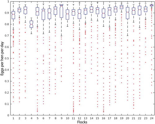
The studied flocks had an average of 8 d labelled as problematic because of drops in production. Certain flocks did not present any decrease in egg production, whereas others presented 33 d labelled as drops in production because of different problems.

The summary statistics for egg production in each flock along with their respective mean and dispersion values visualised in a box and whisker plot are provided in Figure 2. A careful examination indicates that each flock has a different data distribution, which is a favourable situation during the training process because the variability of inputs patterns tends to improve the model generalisations.

Figure 2. Egg production boxplot representing the daily average per bird for each of the 24 flocks analysed in this work.

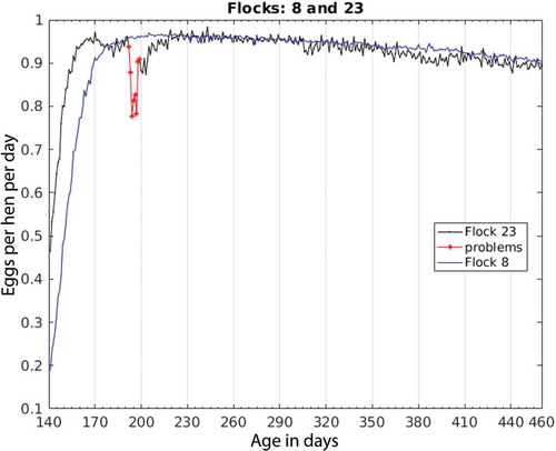
The production of two specific flocks as representative examples of the presence and absence of problems is shown in Figure 3. Flock 8 does not present any anomalies in the production curve, whereas Flock 23 starts production earlier but has a significant drop in egg production between d 191 and 199. This interval was labelled a problem because after d 199, egg production was back to normal.

Figure 3. Daily production per bird in representative flocks number 8 and 23.

The proposed approach for automatic early detection of the anomalies in the production curve of commercial laying hens is based on a classifier combined with a sliding time window, which allows for the detection of anomalies and was based on the study by Bennett and Campbell (2000), who indicated that classification techniques can be used to detect unusual cases.

Data partitioning was performed using a 5-fold cross-validation technique, which guarantees a reduction of possible overfitting (Refaeilzadeh et al. 2009; Kuhn and Johnson 2013). The optimisation of the model was performed by three consecutive steps:

First step: formation of the input patterns

From the preliminary tests, an initial architecture with one hidden layer with 10 neurons, a value of 0.5 for parameter S and a prediction interval equal to one was chosen. The window size and the feature selection threshold were evaluated simultaneously using a grid search technique. An average of 100 runs in the 5-fold cross-validation is shown in Figure 4. The axes of the grid search are the window size and the feature selection threshold.

Figure 4. Grid search for window size and feature selection threshold: (a) accuracy, (b) specificity, (c) sensitivity and (d) positive predictive value.

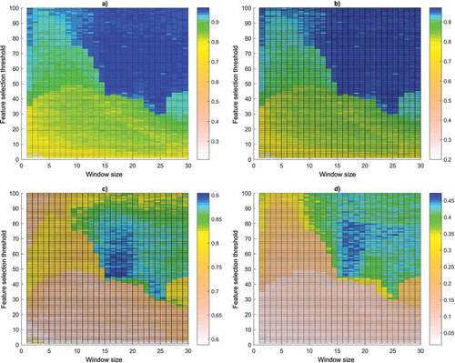
The best ACC results were found with a feature selection threshold greater than 40 along with a window size greater than 15 as shown in Figure 4(a). This finding is similar to what occurs in the case of SPC, which is shown in Figure 4(b). This situation was expected, because the dataset is imbalanced and most targets are negative. Therefore, the influence of these values on the overall ACC of the model is remarkable.

The SEN and PPV results are shown in Figure 4(c,d), respectively. These values express a more marked area of the feature selection threshold between 40 and 70 and the window size between 15 and 20.

Because the selection of relevant features is conditioned by the window size (Frank et al. 2001) and the feature selection threshold, a window size of 18 was chosen along with a feature selection threshold equal to 65. This configuration yields the best results for all performance metrics. The window size and the feature selection threshold, which are far from ideal, display a lower performance, which may be related to insufficient information contained in the selected features or excessive and noisy information for the model. In the model developed by Ramírez-Morales et al. (2016), multiples of 7 for the window size values were required because of the method used by the expert to calculate these features. In the model proposed here, the information contained in the selected relevant features allows for better modelling of the problem without the restriction mentioned before.

The selected relevant features are as follows:

• The number of eggs produced in the first 5 d and the last 4 d of the sliding window.

• The number of dead hens over the past 10 d in the sliding window.

• The number of live hens in the first 14 d of the sliding window.

• All data of cracked eggs in the sliding window.

An illustration of these relevant features is shown in Figure 5, in which the selected features are marked in black.

Figure 5. Selected features with a feature selection threshold of 65 in a window of size equal to 18 d.

In a similar work published by Ramírez-Morales et al. (2016), an early warning classifier for the productive problems of layers was proposed. A poultry expert proposed more than 30 features as inputs to the model. These features went through a process of previous selection and 6 were ultimately selected. The features consisted of indicators calculated from the combination of raw data and other parameters calculated within the sliding time window using a manual trial-error process to choose the best ones. In the current study, an automatic process of selection of relevant features was conducted starting with an analysis of raw data, and an expert was not required.

According to Isabelle Guyon and Elisseeff (2003), the FS is necessary in many cases to prevent overfitting, and it is also related to an improvement of performance and a reduction of computational costs (Saeys et al. 2007; Guyon et al. 2008). For the proposed model, the chosen features correspond to the original raw data, which confer less complexity compared to the required features by Ramírez-Morales et al. (2016). Variables, such as the age of the birds, cumulative mortality, environmental temperature and humidity, were not used as inputs to the model because of their lack of importance according to the automatic FS technique.

Second step: selection of the best ANN architecture

At this stage of the study, 7 architectures were evaluated according to Herrera et al. (2004) and Rivero et al. (2011), who stated that it was necessary to test several different architectures to find the architecture that obtains good results. An ANOVA and Tukey’s Honest Significance Test were performed, and a value of P < 0.01 indicated significant differences (Abdi and Williams 2010).

The window size and the feature selection threshold were fixed in the first step along with a parameter S-value equal to 0.5 and an advance equal to one. A process of testing several predefined architectures was needed to choose the best architecture for the ANN. Among these architectures, the one with the best performance with the test data set was chosen. The evaluated architectures of the ANN are shown in Table 1. It should be noted that none of the two-layer architectures improved upon the results obtained by a single hidden layer architecture consisting of 25 neurons, which showed the best performance metrics.

Table 1. Multiple comparisons of the evaluated architectures.

Network	Accuracy		Specificity		Sensitivity		Positive predictive value
architecture	Mean	STD	Mean	STD	Mean	STD	Mean	STD
[no HL]	0.955^a	0.062	0.956^a	0.063	0.900^a	0.083	0.387^b	0.159
[25]	0.968^a	0.021	0.970^a	0.022	0.880^a	0.057	0.451^a	0.174
[25,25]	0.961^a	0.026	0.962^a	0.027	0.884^a	0.062	0.411^ab	0.178
[25,50]	0.959^a	0.028	0.961^a	0.029	0.884^a	0.058	0.405^ab	0.175
[50]	0.967^a	0.020	0.970^a	0.021	0.879^a	0.059	0.450^a	0.175
[50,25]	0.962^a	0.026	0.964^a	0.027	0.876^a	0.070	0.418^ab	0.180
[50,50]	0.962^a	0.025	0.964^a	0.026	0.876^a.	0.061	0.416^ab	0.175

Means in a row with no common superscript letter differ significantly according to Tukey’s Honest Significance Test for a value of P < 0.01.

ANN training has two sources of random variability: the partitioning of patterns and the initialisation of weights. Consequently, returning the best results of multiple runs is not sufficient to select a proper configuration of parameters. It is recommended to calculate the average and the standard deviation of the performance metrics in all repetitions. Hypothesis tests should be performed to check the significance of differences between ANN configurations (Amiri et al. 2014; Singh et al. 2015; Anwar et al. 2016). Statistically significant differences were not observed for architectures with hidden layers of between 25 and 50 neurons. When deciding between two architectures with statistically equal performances, the less complex architecture is preferred because simpler models tend to be less prone to overfitting. Therefore, to continue with the optimisation, a single hidden layer architecture consisting of 25 neurons was chosen.

Third step: optimisation of the cost-sensitive learning parameter

The third step of the methodology was to tune the value of the parameter S between 0.05 and 0.95 in intervals of 0.05. The ANNs used the window size and a feature selection threshold fixed in the first stage along with the architecture set in the second stage and a prediction interval of 1 d.

The influence of the S-value on the performance metrics of the model is plotted in Figure 6. The line in this figure represents the average of 100 evaluations, and the shaded area corresponds to the standard deviation. The low S-values yielded a high SPC because greater importance was given to the negative patterns; however, the SEN was low. As the S-value increased, the positive patterns had more importance while negative patterns showed reduced importance, which increased the SEN and lowered the SPC. The PPV was also reduced as the S-value increased and the number of false alarms also increased.

Figure 6. Performance chart of the model for different values of the parameter S.

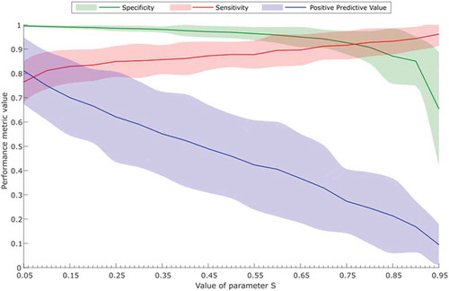
Cost-sensitive learning enabled the model to be fine-tuned to obtain a better response regarding PPV and SEN. The resulting PPV was 0.8125 and 0.7564 for the 0-d and 1-d prediction intervals, respectively, which showed improvements of more than 23% compared to the model published by Ramírez-Morales et al. (2016).

Imbalanced datasets might lead to overfitting of the training algorithms to the most common class and many mistakes in the least common class, leading to a poor generalisation performance (Huang et al. 2006; Blagus and Lusa 2010). A common solution to the overfitting problem in imbalanced datasets is using cost-sensitive learning ANN. This algorithm uses a parameter to weigh the errors in the most infrequent classes (Pazzani et al. 1994; Elkan 2001). Although cost-sensitive learning has attracted the attention of experts in machine learning and data mining, few studies have applied this concept to ANN training (Zhi-Hua and Xu-Ying 2006; Zahirnia et al. 2015).

Similar to other detection problems with low-frequency events, rare examples contain relevant information, such as an early warning system for industrial equipment malfunctioning. The detection of abnormal values in the production curve presents a similar challenge because production drops are usually not observed and few positive cases are found. Vannucci and Colla (2016) argued that traditional classification methods often fail when faced with imbalanced datasets, which is mainly because the misclassification of rare samples is assumed to penalise the misclassification of frequent occurrences. Consequently, classifiers tend to focus on more frequent events. In the present paper, an adjustable parameter S was defined, from which an array of compensation weights was assigned to the unusual patterns. According to Elkan (2001), this adjustment allowed for the fine tuning of the model to obtain a better response regarding PPV and SEN.

A good system must maintain a proper balance between SPC and SEN along with a reasonable value of false alarms. For that reason, an S-value equal to 0.1 was chosen because at this point, SEN was maximised without excessively affecting PPV.

Performance analysis

To evaluate how well the model performed at different prediction intervals, data were reorganised by applying a day shift based on a time delay to the expected outputs (Martinerie et al. 1998; Kapoor and Bedi 2013). Therefore, in the 0-day prediction interval, the targets correspond to the same day of the pattern, whereas in the 5-d prediction interval, the targets correspond to 5 d later in the pattern. A range of prediction intervals was tested from 0 to 5.

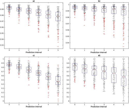
The distribution of performance metrics results in 100 replicates of the 5-fold cross-validation as shown in Figure 7. The mean and standard deviation values for 6 prediction intervals are found in Table 2. The ACC and SPC values are above 0.9758 and 0.9874, respectively. However, a larger mean and a lower dispersion for values of 0 and 1 are observed as shown in Table 2, Figure 7(a,b). On average, the SEN results fall below 0.8 in the prediction interval values ranging from 2 to 5 as shown in Table 2 and Figure 7(c). The PPV value is kept above 0.7 until the prediction interval of 3 d as shown in Figure 7(d).

Table 2. Performance metrics for 5 prediction intervals.

	Prediction interval
Performance	0 d	1 d	2 d	3 d	4 d	5 d
Accuracy	0.9925 ± 0.003	0.9896 ± 0.005	0.9864 ± 0.006	0.983 ± 0.009	0.9797 ± 0.01	0.9758 ± 0.012
Specificity	0.9954 ± 0.003	0.9936 ± 0.005	0.9923 ± 0.006	0.9905 ± 0.009	0.9891 ± 0.011	0.9874 ± 0.014
Sensitivity	0.8639 ± 0.061	0.8169 ± 0.078	0.7362 ± 0.091	0.6643 ± 0.104	0.5795 ± 0.132	0.4821 ± 0.152
Positive predictive value	0.8125 ± 0.119	0.7564 ± 0.14	0.7134 ± 0.166	0.6723 ± 0.19	0.6246 ± 0.22	0.567 ± 0.233

Figure 7. Boxplots of performance metrics for prediction intervals: (a) accuracy, (b) specificity, (c) sensitivity and (d) positive predictive value.

Few previous studies have analysed production parameters to warn of possible problems in egg production; thus, performing comparisons is difficult. The closest work is that of Lokhorst and Lamaker (1996), who proposed an expert system for egg production using a massive amount of data. These data were later turned into relevant information for the model, which obtained an SEN of 0.64 and an SPC of 0.72 in the same day of the anomaly. Compared to these results, the model proposed in this paper obtained an SEN of 0.8639 and an SPC of 0.9954 along with an ACC of 0.9925 and a PPV of 0.8125 for the day prior to the anomaly.

Mertens et al. (2009) also proposed the development of a system based on an intelligent control chart for monitoring the egg production process. This system provided alarms for problems in the production curve for the same day that production dropped. The authors claimed that even when the production curve dropped, this situation remained unnoticed by the layer managers. However, it was not possible to compare this result with that of the present work because the system did not include calculated performance metrics. It should be highlighted that the model presented in the present paper is able to set alarms for good performance metrics up to 3 d before the problem is evident.

Xiao et al. (2011) examined in greater detail the concept of intelligent analysis by developing a software tool that performs statistical analyses of the production curve to identify possible problems. However, these authors did not provide performance metrics to allow for comparisons with our model.

Woudenberg et al. (2014) developed a real-time adaptive egg drop detection method that resulted in a perfect classification of problems for the same day. However, this method was validated in a single flock; thus, measuring its accuracy in a more realistic situation was impossible.

Finally, Ramírez-Morales et al. (2016) presented a model based on support vector machines and features elaborated by an expert. The ACC, SPC, SEN and PPV values were 0.9854, 0.9865, 0.9333 and 0.6135, respectively, and these results correspond to a prediction interval of 1 d before the occurrence of the anomaly. Although the model proposed here reached a lower SEN value of 0.8169, important improvements in the other three performance metrics were obtained (ACC of 0.9896, SPC of 0.9936 and PPV of 0.7564). Therefore, the proposed model moves from expert dependency to expert independency and achieves a greater than 23% improvement in the PPV. This improvement implies a lower number of false alarms and a significant advancement in the practical applicability of continually monitoring poultry production lots.

When the prediction intervals increase, the performance of the model decreases. SEN is the most affected parameter at higher prediction intervals. In the authors’ experience, SEN values above 0.8 are acceptable. Therefore, the optimal prediction interval is 1 d.

Conclusions

The results clearly indicate that anomalies in the production of commercial laying hens can be automatically detected at an early date. The best configuration uses a feature selection threshold equal to 65, a sliding windows size of 18, an ANN with one hidden layer and 25 neurons, and a cost-sensitive learning parameter S-value of 0.1. The model proposed herein can be established as a detector of production drops if it is set for the same day because it has an ACC of 0.9925. Also, it can be configured as an early detector for the previous day because of its ACC of 0.9896. At the farm level, a 1-d advance prediction interval could be useful for on-farm decision-making. This tool would improve the preventive capacity in poultry production systems by providing automatically assisted monitoring as a complement to human observation, and such information is especially useful when handling large animal populations.

Acknowledgements

This work is part of the DINTA-UTMACH and RNASA-UDC research groups. We thank Agrolomas Ltd. for providing access to their data. We acknowledge the support of the Center of Supercomputing of Galicia (CESGA), which allowed the execution of the experimental stage of this work. Ivan Ramirez-Morales and Enrique Fernandez-Blanco would like to acknowledge NVidia because of their support through the grants research programme.

Disclosure statement

No potential conflict of interest was reported by the authors.

Additional information

Funding

This work was partially funded by the Universidad Técnica de Machala, the Xunta de Galicia and the European Regional Development Fund (ERDF) as part of the project GRC2014/049.

References

- Abdi, H., and L. J. Williams. 2010. “Tukey’s Honestly Significant Difference (HSD) Test.” In Encyclopedia of Research Design, 1–5. Thousand Oaks, CA: Sage.
- Amiri, A. S., T. A. Niaki, and A. T. Moghadam. 2014. “A Probabilistic Artificial Neural Network-Based Procedure for Variance Change Point Estimation.” Soft Computing 19 (3): 691–700. doi:10.1007/s00500-014-1293-x.
- Antonov, L. V., K. V. Makarov, and A. A. Orlov. 2015. “Development and Experimental Research on Production Data Analysis Algorithm in Livestock Enterprises.” Procedia Engineering 129: 664–669. doi:10.1016/j.proeng.2015.12.088.
- Anwar, H. M., B. V. Ayodele, C. K. Cheng, and M. R. Khan. 2016. ““Artificial Neural Network Modeling of Hydrogen-Rich Syngas Production from Methane Dry Reforming over Novel Ni/CaFe 2 O 4 Catalysts.” International Journal of Hydrogen Energy 41 (26): 11119–11130.
- Bennett, K. P., and C. Campbell. 2000. “Support Vector Machines.” ACM SIGKDD Explorations Newsletter 2 (2): 1–13. doi:10.1145/380995.380999.
- Blagus, R., and L. Lusa. 2010. “Class Prediction for High-Dimensional Class-Imbalanced Data.” BMC Bioinformatics 11: 523. doi:10.1186/1471-2105-11-523.
- Cameron, A. 2012. Manual of Basic Animal Disease Surveillance. Kenya: Interafrican Bureau for Animal Resources.
- De Vries, A., and J. K. Reneau. 2010. “Application of Statistical Process Control Charts to Monitor Changes in Animal Production Systems.” Journal of Animal Science 88 (13 Suppl): E11–24. doi:10.2527/jas.2009-2622.
- Elkan, C. 2001. “The Foundations of Cost-Sensitive Learning.” International joint conference on artificial intelligence, 2001.
- Flanders, F., and J. R. Gillespie. 2015. Modern Livestock & Poultry Production. Boston, MA: Cengage Learning.
- Frank, R. J., N. Davey, and S. P. Hunt. 2001. “Time Series Prediction and Neural Networks.” Journal of Intelligent and Robotic Systems 31 (1/3): 91–103. doi:10.1023/a:1012074215150.
- Frost, A. R., C. P. Schofield, S. A. Beaulah, T. T. Mottram, J. A. Lines, and C. M. Wathes. 1997. “A Review of Livestock Monitoring and the Need for Integrated Systems.” Computers and Electronics in Agriculture 17 (2): 139–159. doi:10.1016/S0168-1699(96)01301-4.
- Gates, M. C., L. K. Holmstrom, K. E. Biggers, and T. R. Beckham. 2015. “Integrating Novel Data Streams to Support Biosurveillance in Commercial Livestock Production Systems in Developed Countries: Challenges and Opportunities.” Front Public Health 3: 74. doi:10.3389/fpubh.2015.00074.
- Guo, L., D. Rivero, and A. Pazos. 2010. “Epileptic Seizure Detection Using Multiwavelet Transform Based Approximate Entropy and Artificial Neural Networks.” Journal of Neuroscience Methods 193 (1): 156–163. doi:10.1016/j.jneumeth.2010.08.030.
- Guyon, I., S. Gunn, M. Nikravesh, and L. A. Zadeh. 2008. Feature Extraction: Foundations and Applications. Studies in Fuzziness and Soft Computing. Heidelberg: Springer..
- Guyon, I., and A. Elisseeff. 2003. “An Introduction to Variable and Feature Selection.” Journal of Machine Learning Research 3: 1157–1182.
- Hepworth, P. J., A. V. Nefedov, I. B. Muchnik, and K. L. Morgan. 2012. “Broiler Chickens Can Benefit from Machine Learning: Support Vector Machine Analysis of Observational Epidemiological Data.” Journal of the Royal Society Interface 9 (73): 1934–1942. doi:10.1098/rsif.2011.0852.
- Herrera, F., C. Hervas, J. Otero, and S. Luciano 2004. “Un Estudio Empırico Preliminar Sobre Los Tests Estadısticos Más Habituales En El Aprendizaje Automático.” Tendencias de la Minerıa de Datos en Espana, Red Espanola de Minerıa de Datos y Aprendizaje (TIC2002-11124-E):403–412.
- Huang, Y.-M., C.-M. Hung, and H. C. Jiau. 2006. “Evaluation of Neural Networks and Data Mining Methods on a Credit Assessment Task for Class Imbalance Problem.” Nonlinear Analysis: Real World Applications 7 (4): 720–747. doi:10.1016/j.nonrwa.2005.04.006.
- Kalhor, T., A. Rajabipour, A. Akram, and M. Sharifi. 2016. “Modeling of Energy Ratio Index in Broiler Production Units Using Artificial Neural Networks.” Sustainable Energy Technologies and Assessments 17: 50–55. doi:10.1016/j.seta.2016.09.002.
- Kapoor, P., and S. S. Bedi. 2013. “Weather Forecasting Using Sliding Window Algorithm.” International Scholarly Research Network Signal Processing 2013: 1–5. doi:10.1155/2013/156540.
- Kruse, R., C. Borgelt, F. Klawonn, C. Moewes, M. Steinbrecher, and P. Held. 2013. “Multi-Layer Perceptrons.” In Computational Intelligence, 47–81. London: Springer.
- Kuhn, M., and K. Johnson. 2013. Applied Predictive Modeling. New York: Springer.
- Lindsay, D., and S. Cox. 2005. Effective Probability Forecasting for Time Series Data Using Standard Machine Learning Techniques, 35–44. Berlin: Springer.
- Lokhorst, C., and E. J. J. Lamaker. 1996. “An Expert System for Monitoring the Daily Production Process in Aviary Systems for Laying Hens.” Computers and Electronics in Agriculture 15 (3): 215–231. doi:10.1016/0168-1699(96)00017-8.
- Long, A., and S. Wilcox. 2011. “Optimizing Egg Revenue for Poultry Farmers.” Poultry, 1–10. Science.
- Ma, X., Y. Zhang, and Y. Wang. 2015. “Performance Evaluation of Kernel Functions Based on Grid Search for Support Vector Regression.” 2015 IEEE 7th International Conference on Cybernetics and Intelligent Systems (CIS) and IEEE Conference on Robotics, Automation and Mechatronics (RAM), 2015/7.
- Martens, D., and B. Baesens. 2010. “Building Acceptable Classification Models, 53–74. Boston, MA: Springer.
- Martinerie, J., C. Adam, M. Le Van Quyen, M. Baulac, S. Clemenceau, B. Renault, and F. J. Varela. 1998. “Epileptic Seizures Can Be Anticipated by Non-Linear Analysis.” Nature Medicine 4 (10): 1173–1176. doi:10.1038/2667.
- Mertens, K., I. Vaesen, J. Löffel, B. Kemps, B. Kamers, J. Zoons, P. Darius, E. Decuypere, J. De Baerdemaeker, and B. De Ketelaere. 2009. “An Intelligent Control Chart for Monitoring of Autocorrelated Egg Production Process Data Based on a Synergistic Control Strategy.” Computers and Electronics in Agriculture 69 (1): 100–111. doi:10.1016/j.compag.2009.07.012.
- Møller, M. F. 1993. “A Scaled Conjugate Gradient Algorithm for Fast Supervised Learning.” Neural Networks 6 (4): 525–533. doi:10.1016/s0893-6080(05)80056-5.
- Mucherino, A., P. J. Papajorgji, and P. M. Pardalos. 2009. Data Mining in Agriculture. Vol. 34, Springer Optimization and Its Applications. Edited by Panos M. Pardalos. New York, NY: Springer.
- Narinc, D., F. Uckardes, and E. Aslan. 2014. “Egg Production Curve Analyses in Poultry Science.” Worlds Poultry Sciences Journal 70 (04): 817–828. doi:10.1017/S0043933914000877.
- Pazzani, M., C. Merz, P. Murphy, K. Ali, T. Hume, and C. Brunk. 1994. “Reducing Misclassification Costs.” Proceedings of the Eleventh International Conference on Machine Learning, 1994.
- Pica-Ciamarra, U., D. Baker, N. Morgan, and A. Zezza. 2014. Investing in the Livestock Sector: Why Good Numbers Matter, A Sourcebook for Decision Makers on How to Improve Livestock Data. Washington, DC: The World Bank and FAO.
- Ramírez-Morales, I., D. Rivero-Cebrián, E. Fernández-Blanco, and A. Pazos-Sierra. 2016. “Early Warning in Egg Production Curves from Commercial Hens: A SVM Approach.” Computers and Electronics in Agriculture 121: 169–179. doi:10.1016/j.compag.2015.12.009.
- Refaeilzadeh, P., L. Tang, and H. Liu. 2009. “Cross-Validation.” In Encyclopedia of Database Systems, edited by L. Liu and M. Tamer Özsu. 532-538. New York: Springer US.
- Rivero, D., E. Fernandez-Blanco, J. Dorado, and A. Pazos. 2011. “Using Recurrent ANNs for the Detection of Epileptic Seizures in EEG Signals.” 2011 IEEE Congress of Evolutionary Computation (CEC), 2011/6.
- Saeed, K., and S. Václav 2014. Computer Information Systems and Industrial Management: 13th IFIP TC 8 International Conference, CISIM 2014, Ho Chi Minh City, Vietnam, November 5-7, 2014, Proceedings: Springer.
- Saeys, Y., I. Inza, and P. Larranaga. 2007. “A Review of Feature Selection Techniques in Bioinformatics.” Bioinformatics 23 (19): 2507–2517. doi:10.1093/bioinformatics/btm344.
- Samborska, I. A., V. Alexandrov, L. Sieczko, B. Kornatowska, V. Goltsev, M. D. Cetner, and H. M. Kalaji. 2014. “Artificial Neural Networks and Their Application in Biological and Agricultural Research.” NanoPhotoBioSciences 2: 14–30.
- Schaefer, A. L., N. Cook, S. V. Tessaro, D. Deregt, G. Desroches, P. L. Dubeski, A. K. W. Tong, and D. L. Godson. 2004. “Early Detection and Prediction of Infection Using Infrared Thermography.” Canadian Journal of Animal Science 84 (1): 73–80. doi:10.4141/a02-104.
- Singh, P. K., R. Sarkar, and M. Nasipuri. 2015. “Statistical Validation of Multiple Classifiers over Multiple Datasets in the Field of Pattern Recognition.” International Journal of Applied Pattern Recognition 2 (1): 1. doi:10.1504/ijapr.2015.068929.
- Sun, Y., A. K. C. Wong, and M. S. Kamel. 2009. “Classification of Imbalanced Data: A Review.” International Journal of Pattern Recognition and Artificial Intelligence 23 (04): 687–719. doi:10.1142/s0218001409007326.
- Vannucci, M., and V. Colla. 2016. “Smart Under-Sampling for the Detection of Rare Patterns in Unbalanced Datasets.” In Intelligent Decision Technologies 2016, edited by I. Czarnowski, A. M. Caballero, R. J. Howlett, and L. C. Jain, 395–404, Basel: Springer International Publishing.
- Venkatesan, M., A. Thangavelu, and P. Prabhavathy. 2013. Proceedings of Seventh International Conference on Bio-Inspired Computing: Theories and Applications (BIC-TA 2012). Vol. 202, Advances in Intelligent Systems and Computing. India: Springer India.
- Wheeler, E. F., K. D. Casey, J. S. Zajaczkowski, P. A. Topper, R. S. Gates, H. Xin, Y. Liang, and A. Tanaka. 2003. “Ammonia Emissions from US Poultry Houses: Part III–broiler Houses.” Air Pollution from Agricultural Operations-III, Raleigh, NC, October 12–15.
- Woudenberg, S. P., D. Linda Gaag, A. Feelders, and A. R. Elbers. 2014. “Real-Time Adaptive Problem Detection in Poultry.” In Ecai 2014, 1217–1218. Amsterdam: IOS Press.
- Xiao, J., H. Wang, L. Shi, L. Mingzhe, and M. Haikun. 2011. “The Development of Decision Support System for Production of Layer.” Computer and Computing Technologies in Agriculture V, Beijing, October 29-31. Berlin: Springer.
- Zahirnia, K., M. Teimouri, R. Rahmani, and A. Salaq. 2015. “Diagnosis of Type 2 Diabetes Using Cost-Sensitive Learning.” 2015 5th International Conference on Computer and Knowledge Engineering (ICCKE), 2015/10.
- Zhi-Hua, Z., and L. Xu-Ying. 2006. “Training Cost-Sensitive Neural Networks with Methods Addressing the Class Imbalance Problem.” IEEE Transactions on Knowledge and Data Engineering 18 (1): 63–77. doi:10.1109/tkde.2006.17.