Spatial Sorting of Rich Versus Poor People in Jakarta

Abstract

We test an adjusted version of the classic monocentric-city model to explain the spatial sorting of rich versus poor people in Jakarta. We find that in Jakarta (1) the urban rich tend to live in the city centre; (2) because of extreme congestion levels, the elasticity between income and the opportunity cost of time spent commuting is higher than the elasticity between income and demand for larger plots of residential land; and (3) the motorbike is the most important and fastest mode of transport for the urban poor. These findings contrast with existing evidence from the United States. Both the logic of the monocentric-city model and empirical evidence suggest that the urban rich in Jakarta tend to cluster in the city centre. However, empirical evidence also suggests that the sorting of the rich and poor in Jakarta—as indicated by spatial variation in income, expenditure and land prices—depends not only on distance from the city centre but also on other neighbourhood characteristics, especially flood risk, crime rates and the proximity of a commercial area.

Kami menguji sebuah versi modifikasi dari model klasik kota monosentris (classic monocentric-city model) untuk menjelaskan pemilahan spasial golongan masyarakat kaya dan miskin di Jakarta. Kami menemukan bahwa di Jakarta: (1) kaum kaya perkotaan cenderung hidup di pusat kota; (2) oleh karena tingkat kepadatan yang ekstrim, elastisitas pendapatan terhadap biaya kesempatan dari waktu yang dihabiskan untuk melaju lebih besar daripada elastisitas pendapatan terhadap permintaan untuk tanah tempat tinggal yang lebih besar; dan (3) sepeda motor merupakan moda transportasi yang paling diandalkan dan paling cepat bagi kaum miskin perkotaan. Temuan-temuan ini kontras dengan bukti empiris dari Amerika Serikat. Baik logika dari model kota monosentris maupun temuan empiris mengindikasikan bahwa kaum kaya perkotaan di Jakarta cenderung berkelompok di pusat kota. Namun demikian, temuan empiris juga mengesankan bahwa pemilahan antara kaum kaya dan miskin di Jakarta—sebagaimana diindikasikan oleh variasi spasial pada pendapatan, pengeluaran, dan harga tanah—tidak hanya ditentukan oleh jarak ke pusat kota, melainkan juga oleh karakteristik pemukiman, terutama risiko banjir, tingkat kriminalitas, dan kedekatan dengan area komersil.

Keywords:

• urban poverty
• commuting
• public transport
• monocentric-city model
• sorting

JEL classifications:

• O17
• O18
• O53
• P25
• R14
• R21
• R23
• R41

INTRODUCTION

In recent decades, urbanisation has increased more rapidly in the Asia Pacific than in any other region in the world. Larger cities have especially been engines of economic growth and wealth creation yet have had high levels of urban poverty, congestion and segregation of the rich and poor. In this context, we analyse the spatial sorting of rich versus poor people in Jakarta, one of the largest urban areas in the world (Rukmana 2018). Where do the urban poor in this area live, and why? The term spatial sorting refers to the phenomenon in which heterogeneous citizens (households)—who have preferences for consumption, housing and neighbourhood amenities—choose a location within the city to maximise their utility. To date, many urban-location models allow the study of this sorting of residents across space. We base our analysis on the so-called monocentric-city model, pioneered in the 1960s by William Alonso, Richard Muth and Edwin Mills (see Kraus 2008). The model is referred to as the AMM model, and still serves as a benchmark for understanding spatial sorting in urban economics. In short, the model assumes that urban employment is concentrated in a central business district (CBD), while population density, land values and house prices decrease as distance from the CBD increases. The decrease in land prices is predicted to compensate for the costs of longer commutes; individuals thus face a trade-off between their housing costs and commuting costs.

In this article, we use an adjusted version of the AMM model, in which we assume the existence of two income groups (rich and poor) and two modes of transport (motorbike and car). This adjusted version of the classic AMM model has been used to argue that access to public transport is an important factor in explaining where the urban poor live (Glaeser, Kahn and Rappaport 2008; Pathak, Wyczalkowski and Huang 2017; Barton and Gibbons 2017; Brueckner and Rosenthal 2009; Giuliano 2005). For example, using LeRoy and Sonstelie’s (1983) theory on varying transport technologies and income, Pathak, Wyczalkowski and Huang (2017) and Glaeser, Kahn and Rappaport (2008) have shown that if the urban poor are dependent on cheap but slow public transport (in contrast to the urban rich, who can afford expensive, fast cars), the monocentric-city model predicts that the urban poor will tend to concentrate in the city centre, where access to public transport is relatively good and commuting distances to the CBD are relatively short. Glaeser, Kahn and Rappaport (2008) found strong empirical evidence supporting this prediction, for the United States. The question is whether these conclusions lend themselves to generalisations: do they hold outside the United States? For example, Cuberes, Roberts and Sechel (2019) found that in English cities primarily the non-poor cluster near public-transport facilities, contradicting the evidence from the United States. But what about large cities in the global south? Is the intra-urban spatial distribution of the poor in these cities shaped by public-transport access?

Megacities in the global south, such as Jakarta, differ from large cities in rich countries in several relevant aspects (Glaeser and Henderson 2017). First, the combination of high population density, rapid urban growth—driven by economic transformation and rural–urban migration flows—and relatively weak property rights leads to the emergence of informal settlements, a feature which is uncommon in rich countries (Cervero 2013; Gwilliam 2003; Dovey and King 2011). Second, megacities in the global south are some of the most congested cities in the world. Rapid urban growth, together with relatively weak urban-planning structures and practices, has led to inadequate provision of transport infrastructure, including public-transport services, in many of those cities. In response, this has given rise to alternative transport modes such as motorbikes and informal minibus services, which are much less common in richer nations. Third, compared with large cities in rich countries, income disparities and poverty levels tend to be much greater across megacities in the south (Gwilliam 2003; Dovey and King 2011). This translates into, among other things, relatively large intra-urban differences in the perceived value of time, and may thereby alter key assumptions of the monocentric-city model.

Against this background, we present a unique data set for Jakarta that we constructed by combining and processing data from a variety of sources. We first used the data to develop a descriptive empirical analysis of the spatial distribution of income, employment and amenities, as well as commuting behaviour across Jakarta. Second, we used the data to calibrate the adjusted AMM model for the Jakarta metropolitan area and tested its predictions in regard to the spatial sorting of the urban poor in this area. Urban data for Indonesia are not as abundant and reliable as for the United States. Hence, we could not apply the entire estimation strategy used by Glaeser, Kahn and Rappaport (2008), and consequently our regression results are less precise and less comprehensive. Nevertheless, we identified key stylised facts on the spatial distribution of income, employment and land quality as well as mobility behaviour, and we tested the key predictions of the AMM model for Jakarta. In doing so, we can show the possibilities and limitations of existing data sets for empirical urban-economic analyses in Indonesia.

The intra-urban spatial distribution of the urban poor in Jakarta has been implicitly studied by authors who analysed the determinants of the spatial patterns of land prices in the region. For example, using data from 1987–89, Dowall and Leaf (1991) found that infrastructural provision and tenure (through land titles) in Jakarta are important drivers of the land prices. Also, they found that price increases have been consistently greater in suburban areas and for informally occupied plots of land, arising from the massive demand from low-income households for affordable housing. Han and Basuki (2001) observed that variation in land prices in Jakarta is not distributed evenly as a simple function of distance from the CBD: in central Jakarta, one could find cheap land parcels, reflecting the mixture of slums and skyscrapers, while land was more expensive in west and south Jakarta than in north and east Jakarta. At the same time, the authors concluded that spatial variables, especially distance from the CBD, were important in shaping land value patterns in Jakarta, but that the explanatory power of distance declined over time. Lewis (2007) empirically analysed the relationship between residential land prices and distance from the CBD, as well as other pertinent variables, including environmental conditions. Interestingly, he found that, among other things, the land market in Jakarta significantly values environmental conditions, including access to key types of infrastructure (especially water and wastewater facilities) and certain favourable physical characteristics of the property (such as resistance to flooding). Gnagey and Tans (2018) used a hedonic-pricing analysis to study land-price formation across the Indonesian archipelago, including previously unstudied regional property markets. They found that property characteristics, land-ownership status and advertising methods are all statistically significant indicators of land prices.

These studies, however, do not explicitly develop an adjusted AMM model for Jakarta and do not focus on the role of urban transport in explaining the sorting of the urban poor. An interesting study that does use the monocentric-city framework to analyse the link between spatial sorting and the role of public transport in an Asian city was conducted by Li et al. (2019). They looked at the spatial patterns of apartment prices and their association with local attributes in Shanghai, finding that Shanghai’s residential market has a monocentric structure because of the centralised distribution of public-transport facilities and amenities. In addition, they found that structural attributes and accessibility, as well as public and private services, significantly shape the real-estate market in different ways, so as to form a pattern of concentric rings. Interestingly, in the suburbs, good access to bike sharing, bus stops and metro stations is a top preference of apartment buyers.

This paper is organised as follows. In the next section, we list our data sources and discuss how we processed and combined the various data series. We then present a descriptive analysis of the spatial distribution of incomes, employment and amenities across Jakarta, as well as an analysis of commuting behaviour across income groups. Using these stylised facts, we discuss the key features of the monocentric-city model and the adjustments that we think are needed to make the model fit Jakarta. In doing so, we further develop the hypotheses on the expected spatial sorting of the rich and poor. Lastly, we use a regression analysis to estimate the key parameters of the model for the case of Jakarta and to test for its key predictions on the sorting of the urban rich versus the urban poor.

DATA

Spatially explicit data on incomes, employment, amenities and commuting behaviour are not readily available for Jakarta. Hence, we constructed a new data set by combining several existing data sets and data-processing strategies. Our data on commuting flows originate from the 2014 Jabodetabek Commuter Statistics (JKS) survey and the 2010 Commuter Survey (Survey Wawancara Rumah Tangga), conducted respectively by Indonesia’s central statistics agency, Statistics Indonesia (BPS), and the Japan International Cooperation Agency (JICA) in cooperation with the Indonesian Coordinating Ministry of Economic Affairs. Both surveys include data on commuting patterns and household characteristics. The 2014 JKS covered about 5,000 households in Jakarta. JKS provides the most recent data, which is important, as taxi companies Gojek and Grab entered the market in Jakarta in 2011. However, JKS is inaccurate when aggregating data at the subdistrict level, since its sampling framework is not random. Further, BPS records a commuting trip only if the commuter has travelled from one district to another. Thus, all within-district trips are not recorded as commuting trips. The 2010 JICA survey, a household survey covering about 50,000 households in Jakarta, complements the JKS since its sampling framework can be considered more random owing to the high participation of households. The aggregates of income and expenditure per neighbourhood originate from the JICA survey.

A drawback of both these data sets is their relatively high margins of error due to respondents often being unaware of their exact behavioural characteristics, or due to the sensitivity of some topics (such as income), which means that answers to questions related to these topics are relatively unreliable.

Obviously, this is a matter of concern for our analysis, given its focus on incomebased sorting patterns. To address potential bias in our results, we adopted an empirical strategy that incorporates household expenditure and estimates of the tax value of land in Jakarta as proxies for income. To this aim, we used a data set that includes estimates of land prices for Jakarta’s neighbourhoods, constructed by the Jakarta National Land Agency (BPN) in 2016. Even though these land prices are estimates, the data set is not subject to the same sensitivities as the household observations, and it incorporates almost all neighbourhoods in Jakarta. The tax value of land can be seen as a relevant proxy for income under the presumption that the urban poor are not able to afford housing where the price of land is high. Finally, we improved the reliability of the information extracted from the household surveys by comparing data on the tax value of land, income and expenditure.

The data set also prevented us from controlling for amenities that may affect income, land value and commuting behaviour, while time invariance in the data prevented us from conducting a fixed-effects analysis. However, to improve the quality of our regression analysis, we collected data on neighbourhood characteristics that could help to reduce potential endogeneity issues in our regression models. Specifically, we controlled for neighbourhood-specific crime rates, flood risk, public-transport access, population density, open space, slums and commercial areas. Data on crime rates and population density were taken from the data set Districts in Numbers 2004–18, held by BPS in Jakarta. Flood-risk data are open source and were developed in 2013 by Jakarta’s Special Capital Region (DKI) Regional Disaster Management Agency (BPBD) and OpenStreetMap (OSM).¹ We checked the reliability of our data and our results with a local flooding expert. Google Maps was used to obtain data on public-transport access. Information on slum areas in 2015 was provided by the National Land Agency (BPN) in Jakarta. Information on access to commercial areas was collected from OSM data for 2017. A description and summary of all variables included in the analysis can be found in table A1.1 in the online appendix.²

In the next section, we use our data to document several stylised facts about the spatial distribution of incomes, land prices and mobility behaviour across income groups in Jakarta.

DESCRIPITVE ANALYSIS

Incomes

We start our descriptive analysis by presenting in figure 1 income distribution as a function of distance from the CBD for three cities: Jakarta, Los Angeles and Chicago.³ To facilitate comparison across these cities, we indexed the incomes such that income at each CBD had an index value of 100.

FIGURE 1 Income and Distance from the CBD, for Four Cities

Source: Data for Jakarta are from the 2014 JKS survey. Data for Chicago, Philadelphia and Los Angeles were taken from Glaeser, Kahn and Rappaport’s (2008) study.

Note: Distance from the CBD is the Euclidean distance. Income values in rupiah were converted into US dollars by using the purchasing-power parity of 2014 (OECD 2019). The slopes were divided by the average income at zero distance, and multiplied by 100. As the 2014 JKS data are unreliable when aggregated at the neighbourhood level, this graph was plotted using all individual household observations and the distances of the households from the CBD, without aggregating households at a neighbourhood level. The geo-reference is the residential neighbourhood.

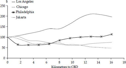
Figure 1 shows that income and distance from the CBD in Jakarta have a negative relationship: the urban rich tend to cluster near the CBD. Hence, the assumption of the classic monocentric-city model that the urban poor cluster in the city centre does not seem to hold for Jakarta. In contrast, the income distribution function in Los Angeles follows the pattern typical for a monocentric city in the United States: the poor concentrate in the city centre, and incomes rise with distance from the CBD. Henderson and Kuncoro (1996) argued that if one were to study Jakarta’s metropolitan area, one would find that the city has a more polycentric structure. It is important to keep this in mind when analysing Jakarta. In Chicago and Philadelphia, incomes first fall and then increase as the distance from the CBD increases. Glaeser, Kahn and Rappaport (2008) stated that this difference might exist because Los Angeles is a relatively new city where people are more accustomed to using automobiles. In contrast, the city centres of Chicago and Philadelphia have a much more historical character and seem to attract wealthier households. This pattern can also be found in many European cities with historical city centres.

Land Prices

To illustrate the location behaviour of people in Jakarta, we present in figure 2 the estimated tax value of land per square metre for neighbourhoods, in combination with flood vulnerability. The triangle in the centre represents the CBD. Most of Jakarta’s employment is centred in and around this triangle. The tax values indicate neighbourhood prosperity; more-developed areas have higher land values and attract wealthier households. According to figure 2, land prices are highest in and around the CBD, which includes wealthy subdistricts such as Menteng, Tebet, Setiabudi, Tanah Abang and Senen. Other high-tax areas are Kebayoran Baru, Kelapa Gading and Pantai Indah Kapuk. Lower land values seem to be predominant in the north-east, north-west and south of Jakarta. Large slums are most predominant in the north.

FIGURE 2 Land Tax Values and Flood-Vulnerable Areas in Jakarta, 2016

Source: BPN and BPBD DKI Jakarta.

Note: Tax values represent the estimated average tax value per square metre as determined and collected by the BPN when a party buys or sells a plot of land. The tax value is in Indonesian rupiah (million), where $1 dollar is equivalent to about Rp 14.08. For instance, the mean tax value of land in Jakarta’s wealthiest subdistrict, Menteng, is estimated to be $2,904 per square metre; converting this using the purchasing-power parity gives $10,113 per square metre (OECD 2019). Flood-vulnerable areas are defined based on information provided by the villages about flooding. The online appendix contains a colour map (figure A1) that more clearly outlines Jakarta’s flood-vulnerable areas and shows its slum areas.

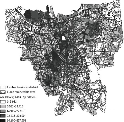
Figure 2 also shows that, as expected, most of the areas that are vulnerable to flooding have relatively low tax values. According to the World Bank (2011), residents living in slum areas are the most affected by floods, as many informal settlements have developed in floodplain areas.

Commuting Behaviour

Besides being highly vulnerable to flooding, Jakarta struggles with a series of transport challenges, including extreme traffic congestion (Asri and Hidayat 2005). To improve mobility, the government has developed several public-transport lines. For instance, the local government set up the Transjakarta bus rapid transit (BRT) system in 2004. Jakarta also has several railway networks. The most extensive is the Electric Rail Train (KRL) Commuter Line, originally operated by a Dutch colonial railway company (Farda and Lubis 2018). Besides public transport, commercial taxi services such as Gojek and Grab are common in Jakarta (Von Vacano 2017).

To understand the relationship between transport use and the sorting of the urban poor in Jakarta, we need to establish key characteristics of the three mostused transport modes: car, bus and motorbike.⁴ To this aim, we report in table 1 some key descriptive statistics for each of these transport modes, based on the survey data discussed in the previous section.⁵ The statistics in table 1 indicate that the car is the most expensive mode of transport. Average income, education level and age are highest for car commuters, suggesting that the wealthy travel by car. This paper classifies the urban poor as individuals earning less than the 2015 minimum wage of Rp 2.7 million (Nababan 2017). The median income is Rp 2.8 million for motorbike users and Rp 2.85 million for public-transport users; hence, almost half of the commuters can be characterised as urban poor. The ability of the urban poor to travel by motorbike contradicts the assumption by Glaeser, Kahn and Rappaport (2008) that the urban poor rely solely on public transport for travel. The average commuting distance is shortest for people who use motorbikes, and longest for those who use public transport. In addition, average travel time is shorter for motorbike users than public-transport users. The gender variable indicates that mainly males commute, regardless of the transport mode. However, the share of females who use cars or public transport is slightly higher than the share who use motorbikes. The average education level is highest for car commuters.

Table 1. Descriptive Statistics of Commuters and Travel, for Selected Transport Modes

Source: JKS (2014).

Notes: ^a The values of the gender variable should be interpreted as the fractions (presented as decimals) of the commuters who are female. ^b The education-variable values are based on an index that is split into four categories: (1) no education through to primary education; (2) middle school education; (3) high-school education; and (5) post-high-school education, such as college. ^c Daily cost of transport accounts for the commuting costs to go to and from work.

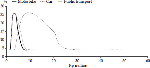
To give further insights into the relationship between income and the use of transport modes, figure 3 illustrates the distribution of income, for each transport mode. The figure shows that, at an income level of about Rp 4 million, the percentages of motorbike and public-transport commuters decline, while the percentage of car commuters increases. Commuters seem to substitute motorbikes and public transport for cars when their income increases. The income pattern of public transport and motorbike commuters resembles that of a normal, bell-shaped distribution, with a slightly longer right tail.

FIGURE 3 Proportion of Commuters Using Each Mode of Transport, with Respect to Income in Jakarta

Source: JKS (2014).

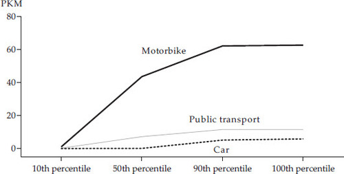
To illustrate the relative importance of each of these transport modes with respect to income, figure 4 plots the cumulative passenger kilometres (PKM) for the three modes. The PKM can be understood as the total kilometres travelled by the users of each mode. In figure 4, income is grouped by percentiles of commuters. The figure shows that the motorbike is the preferred transport mode of about 60% of Jakarta’s daily commuters. It is responsible for about 80% of the total PKM and is the predominant transport mode for lower-income groups. The steepest increase in motorbike use in terms of PKM occurs between the 10^th percentile and the 50^th percentile of income—that is, at relatively low levels of income. Car and publictransport use is more evenly distributed over the income percentiles.

FIGURE 4 Relationship between Millions of Cumulative Passenger Kilometres and Income Percentiles, by Transport Mode in Jakarta

Source: JKS (2014).

Relative to the income earned by users of each transport mode, figure 5a shows the average distance travelled, and figure 5b the average time spent travelling. Figure 5a indicates that the motorbike is used mostly by lower-income groups for distances between 10 and 15 kilometres. Furthermore, the figure shows a negative relationship between income and distance from work for car commuters, and a positive relationship between income and distance from work for public-transport commuters. That is, as income increases, the commuting distance for car commuters decreases, while the distance for public-transport commuters increases. Interestingly, the figure also shows that, at higher income levels, the longest distances are travelled by public transport and not by car, which clearly contrasts with findings of LeRoy and Sonstelie (1983).

FIGURE 5 Relationship between Transport Modes and Income in Jakarta

Source: JKS (2014).

Notes: The graph corresponds to data from 2014; only incomes up to Rp 31 million per month are included.

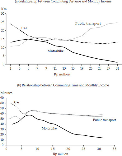
Figure 5b shows that the slope of the travel time to work for public-transport users and that for car commuters begin to run parallel as income increases, after about Rp 6 million per month. Figure 5a suggests that public-transport commuters also begin to travel longer distances than car users after the income level of Rp 6 million. Low-income public-transport commuters have shorter commuting distances on average than low-income car or motorbike commuters. However, the commuting time for these public-transport commuters is not the shortest. These two phenomena suggest the presence of economies of scale for public-transport commutes; distance and time do not increase proportionally, creating an incentive to travel by public transport when distance increases—a phenomenon that contrasts with evidence from cities in the United States and many other rich countries.

Spatial Sorting

Together, these observations lead to the conclusion that in Jakarta the urban rich tend to live in the city centre, presumably because of good land quality and the high travel-time costs of commuting by car; hence, wealthy inhabitants have an incentive to live near their place of employment to reduce travel-time costs. Also, we conclude that public transport has a comparative advantage for long-distance commutes, whereas the motorbike is frequently used for relatively short travel distances (up to 15 kilometres). This suggests that lower-income commuters in Indonesia have less incentive to live near Jakarta’s city centre than, for instance, commuters in the United States have to live near Los Angeles. The mobility advantage of the car—as presumed by Glaeser, Kahn and Rappaport (2008)—is clearly undermined in Jakarta by the presence of motorbikes. However, figure 5a also suggests that the urban rich do not necessarily have the shortest commutes; otherfactors are thus likely to be important in understanding Jakarta’s income-based sorting patterns. These stylised facts tell us how we might adjust the monocentric model in order to apply it to the case of Jakarta. This is the topic of the next section.

AN ADJUSTED MODEL OF URBAN SORTING

As indicated, our analysis finds its roots in the classic monocentric-city model, or AMM model. The model assumes a circular city in a featureless plain, populated by N identical individuals whose utility depends on a consumption mix of (multidimensional) housing services, q, and a composite of other goods, c. Everyone is assumed to commute daily to the CBD, where each person works to receive a wage, w. An individual who lives at radial distance d from employment in the CBD faces a daily commuting cost of td, where t > 0 is the commuting cost per unit of distance, and pays the rental price r(d) (per unit) of housing q. An individual’s objective is to maximise the utility function u(q,c), subject to the following budget constraint:

The model is solved by deriving the optimal individual budget allocation between housing q and the composite consumption good c (the numeraire) at each location d to obtain house prices r. This problem of choice is equivalent to maximising u(q, w − td −rq) with respect to q. The first-order condition of this problem yields demand for housing at each location according to the following:

which states that the marginal utility of more housing per amount spent should be equal to the marginal utility of the numeraire consumption good. Using the budget constraint (equation 1), the demand for the numeraire c(d) can be recovered as a function of the Marshallian demand for housing, according to c(d) = w − td − r(d) q(d). In equilibrium, all individuals must obtain the same level of utility u; hence, u(q(d), w – td – P(d)q(d)) = ū Totally differentiating this equation with respect to d, by using equation 2 and the envelop theorem, yields the following:

Equation 3 describes the Alonso–Muth condition that, in equilibrium, if a resident moves marginally away from the CBD, the cost of the current housing consumption q falls just as much as the commuting cost t increases. In other words, the monocentric-city model predicts that house prices will fall with distance from the CBD to compensate for the costs associated with longer commutes; a trade-off thus exists between house prices and commuting costs. Hence, equation 3 is the bid–rent gradient, which defines house (land) prices as a function of distance from the CBD. The underlying idea here is spatial equilibrium: because households have a location choice and are assumed to be homogeneous, the same utility level must be realised at all residential locations; if it is not, individuals will move location to increase their utility. The mechanism for satisfying the equal-utility condition is spatial variation in the price of housing. Consequently, the house-price function of equation 3 equals the bid–rent function of households in a city.

This classic version of the monocentric-city model has been used to develop, for example, polycentric models (Madariaga, Martori and Oller 2013). Also, the assumptions in the literature on urban economics that households (workers) and transport costs are homogeneous—that is, they can be represented by one household and one transport mode—have been relaxed. As noted in the introduction, to frame our empirical analysis, we used an adjusted version of the classic AMM model, in which we assumed the existence of two income groups (rich and poor) and two modes of transport (motorbike and car), following earlier work by Glaeser, Kahn and Rappaport (2008).

Let us define rich or poor people’s income as w_rich or w_poor and their opportunity costs of time as k_rich or k_poor, and let us assume for simplicity that housing (land) consumption of the rich or poor is fixed at q_rich or q_poor. The steepness of the bid–rent gradient (equation 2) determines which group lives closest to the CBD. The group with the steeper bid–rent gradient will be willing to pay more for land closer to the CBD. If both income groups have the same transport costs, the model predicts that the urban poor will live closest to the CBD only if the elasticity of housing consumption with respect to income is greater than the income elasticity of commuting time costs:

where the income elasticity of demand for housing (land) with respect to income w is

and the income elasticity of the time cost of commuting is

However, this condition changes if the two groups have different transport costs. Glaeser, Kahn and Rappaport (2008) introduced two transport modes: public transport (the bus) that is slow but cheap, and private transport (the car) that is fast but expensive. They showed that if poor people choose public transport (given its low fixed cost compared with the car), and rich people choose the car (given their higher opportunity costs of time), the monocentric-city model predicts that the urban poor will have a steeper bid–rent gradient than the rich and will live closer to the CBD if

This condition thus states that the chance that the urban poor will live close to the CBD depends not only on the elasticity of housing consumption with respect to income and the income elasticity of commuting time costs , but also on the comparative advantage of the urban rich in using the car. Glaeser, Kahn and Rappaport (2008) argued that this is a more realistic condition to hold than that of equation (4). This condition also implies the existence of a break-even distance (d*) where the lower variable (time) cost of a car exactly offsets its higher fixed cost. Finally, they argue that if (easy) access to public transport is restricted to the city centre—as is often the case in US cities—the tendency for the urban poor to cluster in and near the city centre is further increased. Indeed, when putting the adjusted AMM model to the test across US cities, Glaeser, Kahn and Rappaport (2008) found robust empirical evidence that transport-mode choice plays a key role in explaining why the urban poor tend to live in the city centre.

To test whether transport-mode choice can also explain where the urban poor live in Jakarta, we need to especially consider three features of Jakarta that set it apart from the average US city: (1) the omnipresence of motorbikes; (2) its severe level of congestion; and (3) its high level of income inequality (Yusuf, Sumner and Rum 2014).⁶ As regards the first feature, earlier we documented that the motorbike is the predominant transport mode for lower income groups and that the ability of the poor to afford a motorbike greatly affects their mobility, and thus undermines the assumption in the work by Glaeser, Kahn and Rappaport (2008) that the poor depend on access to public transport to satisfy their transport demand. In fact, in contrast to US cities, the key divide in transport modes in Jakarta is between the car and the motorbike rather than between the car and the bus (for comparison, see Fevriera, de Groot and Mulder 2021). Given the affordability and speed of motorbikes, the area where public transport has a comparative advantage over cars in Jakarta would be much smaller than in a city where cars compete more directly with public transport. The motorbike is more flexible in traffic and a cheaper transport mode than the car, offering an additional alternative to public transport. In other words, the urban poor in Jakarta are likely to have a much flatter bid–rent function than the urban poor in most US cities. The logic of the AMM model then predicts that poverty is less clustered in Jakarta, since the residential choice of the urban poor is less restricted by the need for short commutes. Further, the assumption that public transport has a comparative advantage for short commutes is unlikely to be relevant in Jakarta, as the descriptive statistics indicate that the commuting time for public transport does not increase proportionally with distance. By contrast, public transport might have a comparative advantage for long-distance commutes. The idea that there is a break-even distance where commuters substitute between the car, the motorbike and public transport is therefore less likely to hold for Jakarta than for the average US city.

As regards the second feature, in the TomTom Traffic Index of 403 cities for 2018, Jakarta is ranked number 7 in terms of congestion level; in comparison, the highest-ranked US cities in this index are Los Angeles, ranked 24, and New York, ranked 42.⁷ The extreme level of congestion in Jakarta has implications for the assumption about commuting costs in relation to the value of time. It implies that even for people travelling by car, the cost of time makes up a large part of the variable commuting cost. This leads to the hypothesis that distance from the place of employment is a more important factor for residential choice in Jakarta than in US cities, which have less traffic congestion on average. The validity of this hypothesis is of course subject to differences in the opportunity cost of time between the United States and Jakarta. Given the relatively lower average wage level in Jakarta, it seems logical to assume that the opportunity cost of time is lower on average in Jakarta than in the United States. However, the hyper-congestion in Jakarta affects car drivers the most and our data indicate that, in contrast to the United States, commuting by car in Jakarta is predominantly reserved for the higher-income groups—implying that the difference in the opportunity costs of time between car drivers in the United States and in Jakarta may not be all that great.

Finally, the huge income disparities in Jakarta imply that differences in opportunity cost between the urban rich and poor are much larger in Jakarta than in most US cities.⁸ Therefore, it is likely that in Jakarta the elasticity between income and demand for land is lower than the elasticity between income and the opportunity cost of time spent commuting. This contrasts with equation 4, which needs to change into the following:

Given the assumption that the use of relatively fast motorbikes gives the urban poor a mobility advantage over the urban rich, who prefer using cars even though they are slower, equation 5 would then change into the following:

This condition would imply that the rich prefer a short commute rather than a large house, since they value their time more than their consumption of land; their bid–rent function will thus be steeper. If, at the same time, the bid–rent function of the urban poor flattens because of their use of motorbikes, the AMM model predicts that the rich will cluster in and around the CBD, whereas the urban poor will cluster on the outskirts of Jakarta where land prices are lower and commuting distances longer—the opposite of what has been found for the United States. The remainder of this paper is devoted to testing these predictions.

CALIBRATING AND TESTING THE MODEL

In this section, we use regression analysis to calibrate the adjusted monocentriccity model for Jakarta, in order to examine to what extent the predictions of the model hold for Jakarta. Recall that at the core of the monocentric-city model is the argument that the urban sorting patterns of rich versus poor people can mainly be explained by differences between each group’s demand for land and the opportunity cost of time. More specifically, as argued in the previous section, the logic of the model implies that, for the urban rich to live close to the city centre, a necessary condition is that the elasticity of housing consumption with respect to income is lower than the elasticity of the opportunity cost of time spent commuting with respect to income (see equations 4 and 4’). To test for this condition in the Jakarta context, we first estimated the elasticity of demand for housing with respect to income, as did Glaeser, Kahn and Rappaport (2008). We used two techniques to estimate this coefficient. The first is an ordinary least squares (OLS) estimation, controlling for household size (equation 5). The second is a semi-parametric estimation (equation 6). This model allows for any form of the unknown function of the logarithm of expenditure, while household size is included linearly. Given our data restrictions, we measured housing consumption in terms of square metres of floor area rather than in terms of housing prices. We thus first conducted the following OLS estimation:

followed by this semi-parametric estimation:

The unit of observation is individual households (i), with the average monthly household expenditure in rupiah serving as a proxy for income, and with X being the household size and ϵ the error term. The results of this regression are presented in table 2 (columns 1 and 2), alongside the corresponding results from Glaeser, Kahn and Rappaport (2008) (columns 3 and 4) to facilitate comparison.⁹

Table 2. Estimations of Income Elasticity of Demand for Land

Source: JKS (2014) for columns 1–2; Glaeser, Kahn and Rappaport (2008) for columns 3–4.

Notes: Robust standard errors are in parentheses. Household is the unit of analysis. The demographic control variable is household size. OLS stands for ordinary least squares; IV stands for instrumental variable.

^a For apartments and single detached dwelling.

^b In the JKS of 2014, income was equated to expenditure.

* p < 0.10; ** p < 0.05; *** p < 0.01.

Table 2 shows that the elasticity of demand for housing with respect to income in Jakarta is 0.7 for the OLS estimation, which is higher than the elasticity coefficient estimated by Glaeser, Kahn and Rappaport (2008). The semi-parametric regression gives an elasticity of 0.56, which is more compatible with the analysis by Glaeser, Kahn and Rappaport (2008).¹⁰ That the elasticity coefficient is slightly higher in Jakarta could be explained by the fact that the urban poor in Jakarta face more severe income constraints than the urban poor in the United States and thus can afford only small houses in densely populated areas such as slums. It thus may not necessarily be the urban rich who have a high demand for housing but rather the urban poor who demand small settlements owing to income constraints. Nevertheless, for Jakarta, the estimated coefficient is smaller than unity, implying that the demand for housing in Jakarta is moderately inelastic: a 1% increase in income (expenditure) leads to a less than 1% increase in demand for housing (floor area). It should be noted that owing to data constraints, the coefficients cannot be interpreted as causal effects. The results provide insights into the differences between our analysis and that by Glaeser, Kahn and Rappaport (2008). Our empirical strategy is similar to theirs but with multiple data constraints.

Data limitations prevented us from estimating the elasticity of the opportunity cost of time with respect to income for Jakarta. For the United States, Glaeser, Kahn and Rappaport (2008) used a benchmark value of 0.75 for this elasticity. This value is slightly higher than the estimated elasticity of demand for housing with respect to income in Jakarta (see table 2). We are, however, inclined to think that the true elasticity of the opportunity cost of time with respect to income in Jakarta is higher than in the United States, owing to the relatively large within-city differences in income between Jakarta and the average US city. Consequently, it is indeed likely that equation 4’, rather than equation 4, holds in the context of Jakarta: the elasticity of demand for land with respect to income is likely to be smaller than the elasticity of the cost of time spent commuting with respect to income. In other words, the value of time is likely to be a more important determinant of residential choice than the demand for land. According to the AMM model, this would mean that the urban rich prefer a short commute rather than a large house since they value their time more than their consumption of land; their bid–rent function will thus be steeper. As a result, the AMM model would predict that in Jakarta the urban rich live in the city centre, whereas the urban poor cluster on the outskirts of the city. Indeed, in figure 1 we observed a negative relationship between income and distance from the CBD in Jakarta: the urban rich tend to cluster near the CBD. However, our descriptive analysis (see figure 2, for example) also showed that the urban poor live not only at the edges of the city, but also in other areas, including near the CBD.

Next, we test for the assumption in the model by LeRoy and Sonstelie (1983) that the rich predominantly travel by car, while the poor travel by public transport. To establish the choice of transport mode as a function of commuter characteristics in Jakarta, we estimate the following multinomial logistic model by the following equations:

with the dependent variable defined as the logarithm of the probability of individual i choosing specific transport mode j. We distinguish three transport modes—motorbike, car and public transport—where motorbike is determined as the baseline transport choice. The variable X corresponds to a vector of individual characteristics of commuter i, including income, college degree, gender, age and distance from work. The results of this estimation are presented in table 3.

Table 3. Relationships between Selected Transport Modes, and Commuter and Travel Characteristics

Source: JKS (2014).

Notes: The values of the coefficients are interpreted in log odds and thus need to be transformed before one can interpret them as marginal effects. Standard errors are in parentheses. The sample included commuters between the ages of 14 and 69 who commuted within Jakarta and earned a monthly income. Individual commuter is the unit of analysis. Income is specified in millions of rupiah, distance from work is in kilometres and college degree is a dummy variable that equals 1 if the commuter has a college degree or higher. Gender is a dummy variable that equals 1 if the respondent is female. The coefficients for the car and public-transport variables are relative to those for the motorbike (the baseline). For detailed variable descriptions, see online appendix table A1.1.

* p < 0.10; ** p < 0.05; *** p < 0.01.

The results suggest that for each unit of increase in income, age and distance, the logarithm of the odds ratio (log odds) that an individual will choose to commute by car increases, relative to the odds that the individual will choose to commute by motorbike. The same holds for public transport, although the strength of the prediction is not as strong as that for the car. Further, being female and having a college degree also decrease the log odds of choosing a motorbike over public transport or a car. These findings could be explained by the perception that the motorbike is a relatively unsafe, low-status travel mode, making it less attractive for the urban rich and vulnerable commuters. The positive coefficients for travel distance and the car and public transport suggest that motorbikes are considered less suitable for long-distance commutes, presumably because of exposure to pollution and a lack of comfort. In conclusion, our evidence supports the observation that the motorbike is primarily used by low-income commuters; the motorbike is an important mode of transport for the urban poor, which indeed implies that they are less dependent on public transport than the urban poor are in the United States. We continue our analysis by testing the assumption by Glaeser, Kahn and Rappaport (2008) that the rich have a mobility advantage over the poor, in terms of the difference in travel-time cost between the rich and poor. The underlying assumption is that the rich travel by car (expensive but fast), while the poor travel by public transport or motorbike (cheap but slow). We test this assumption for Jakarta by estimating, across individuals i, the equation

in which m is the mode of transport (motorbike, car or public transport), time to work is defined in minutes, and distance from work is measured in kilometres. The data source is again the JKS of 2014, and we include only commuters travelling up to 16.1 kilometres, to make the analysis more compatible with that by Glaeser, Kahn and Rappaport (2008).¹¹ We present the results of this regression in table 4, again in comparison with the findings by Glaeser, Kahn and Rappaport (2008) for the United States in order to allow understanding of the differences between cities in the United States and Jakarta. The findings should not be interpreted as showing causal relationships.

Table 4. Travel Time per Transport Mode

Sources: JKS (2014) for the data on Jakarta, and Glaeser, Kahn and Rappaport (2008) for the data on the United States.

Notes: Robust standard errors are in parentheses. The unit of analysis is an individual living and working in Jakarta where the commuting distance does not exceed 16.1 kilometres.

* p < 0.10; ** p < 0.05; *** p < 0.01.

The results in table 4 indicate that the average speed travelled while commuting is about 24 kilometres per hour for the motorbike (2.5 minutes per kilometre), 23 kilometres per hour for the car (2.6 minutes per kilometre) and 19 kilometres per hour (3.2 minutes per kilometre) for public transport. The estimates for the United States, as presented in table 4, indeed suggest that, across US cities, car commuters have a substantial mobility advantage over public-transport commuters: a car is about twice as fast as public transport for commuting. In contrast, our estimation results suggest that the difference in the variable cost of time between the car and public transport in Jakarta is not as great as in the United States. Further, the motorbike is the fastest transport mode for commuting. Obviously, this is because of Jakarta’s high level of congestion. Also, our results clearly support the observation that the motorbike is a faster mode of transport than the car: the estimated variable travel time for the motorbike is less than that for the car. Presumably, this is because the motorbike is more mobile in highly congested traffic than the car.

In addition, table 4 shows that in Jakarta the fixed time cost for travelling by motorbike, car and public transport are 16.00, 24.91 and 19.18 minutes, respectively. The relatively low fixed time costs for the motorbike suggest that this mode of transport is more suitable for short-distance commutes than the car. Further, in Jakarta the car has the highest fixed costs, unlike in the United States, where the car has the lowest fixed costs. The fixed time cost of public transport can be interpreted as the waiting time for a bus or train. The results suggest that the fixed cost of being stuck in traffic in a car is higher than the cost of waiting for a bus or train: these findings differ from those for the United States.

Recall from equation 5 that the adjusted AMM model with two modes of transport yields the existence of a break-even distance (d*) where the lower variable (time) costs of a certain transport mode exactly offset its higher fixed cost. It is safe to conclude that our analysis supports the anecdotal evidence that motorbikes indeed are the fastest mode of transport on average in Jakarta. This finding further strengthens the notion that in Jakarta the urban rich have a relatively strong preference to live near the city centre. We concluded that the urban rich in Jakarta tend to prefer the car over the motorbike (see table 3), and that their value of time is likely to be an important determinant of residential choice, since the elasticity of the time cost of commuting with respect to income is probably relatively high (see table 2). If the car then is slower than the motorbike, the notion of spatial equilibrium requires that the urban rich can maintain their utility level only by limiting their commuting distance—in line with equation 5.

Obviously, location decisions (of the urban rich) depend not only on commuting time or distance but also on location fundamentals such as the quality of the neighbourhood. Hence, to further investigate the relationship between household income (expenditure) and location choice, we developed a regression approach in which we related household expenditure and land price to location in terms of distance from the CBD, public-transport access and several neighbourhood characteristics. Our approach is inspired by the piecewise linear-regression approach of Glaeser, Kahn and Rappaport (2008); we estimated the relationship between income and distance from the CBD across n neighbourhoods,¹² and we did so in steps, with each step including more control variables to reduce potential endogeneity among the regressors. The overall estimation equation is defined as

where the dependent variable (y_n) is the logarithm of the average aggregate of income,¹³ expenditure or land price at the neighbourhood level;¹⁴ and distance is the Euclidean distance from the CBD for neighbourhood n in kilometres, which includes three spline coefficients regarding distance. We consider distances of less than or equal to 5 kilometres, 5–10 kilometres and more than 10 kilometres. Where x^k2 and x^k3 define the threshold distances (5 and 10 kilometres, respectively), x_k2 is a dummy variable that equals 1 if the distance is between 5 and 10 kilometres, and x_k3 a dummy that equals 1 when the distance is more than 10 kilometres. D_b is a dummy variable for bus stop and equals 1 if neighbourhood n features access to a bus stop within 1 kilometre, and 0 otherwise. D_r is a dummy variable for railway station and equals 1 if neighbourhood n has access to a railway station within 1 kilometre, and 0 otherwise. Values for both the distance variable and these two dummy variables were captured by using zonal statistics in geographic information systems (GIS). The variable flood is a dummy variable that equals 1 if neighbourhood n is vulnerable to floods and 0 otherwise; non-residential areas are excluded. Finally, X is a vector of control variables, including indicators for slum areas, crime rates, open spaces, commercial areas and population density. We capture slum areas using a dummy variable that equals 1 if neighbourhood n borders a slum area;¹⁵ crime rate is defined as the logarithm of total criminal offences in a neighbourhood (village tract) in 2010; open space is defined as the logarithm of the amount of open space at the subdistrict level; and commercial area is captured by a dummy variable that equals 1 if the neighbourhood includes any commercial area. To measure public-transport access, we focused on the KRL Commuter Line and the BRT system.¹⁶

The regression results of this framework are presented in table 5. We only present the results for regressions with expenditure and land price as the dependent variables; the results for the regressions with income as the dependent variable confirm the other results and are presented in table A1.6 in the online appendix.

Table 5. Effects of Neighbourhood Characteristics on Neighbourhood Expenditure and Land Price

Notes: Robust standard errors are in parentheses. The unit of observation is the village tract. The dependent variables are the logarithm of village tract expenditure (source: 2010 JICA survey) and the logarithm of the estimated tax value of village-tract land (source: BPN (2016)). Values for all non-dummy variables are in logarithmic form. The BRT system dummy and KRL dummy equal 1 if the village tract is within 1 kilometre of a public-transport station; only transport lines that were working in 2010 are included. The dummy variable slum equals 1 if the village tract borders a slum area. The dummy variable flood equals 1 if the village tract is affected by floods. For further variable descriptions, see online appendix table A1.1. * p < 0.10; ** p < 0.05; *** p < 0.01

The regression results in table 5 show that both expenditure and land price decrease with distance from the CBD. As we estimate the distance coefficients using a piecewise linear spline regression, we need to establish the change in slopes for the varying distances (less than or equal to 5 kilometres, between 5 and 10 kilometres, and more than 10 kilometres). The distance coefficients in column 3b suggests that a 1% increase in distance from the CBD leads to a land-price decrease of 0.186% for neighbourhoods within 5 kilometres of the CBD, a decrease of 0.252% for subdistricts within 5 to 10 kilometres of the CBD and a decrease of 0.504% for subdistricts more than 10 kilometres from the CBD.As regards expenditure, however, the effect ceases to be statistically significant once we control the regression for neighbourhood characteristics.

In addition, the results clearly indicate that public-transport access positively correlates with land prices. We find that a village tract within 1 kilometre of access to a BRT faces a 16.1% higher land price and a 16.8% higher land price if the village tract has access to the KRL Commuter Line. Clearly, there exists an incentive to live in the vicinity of public transport. As regards the other neighbourhood characteristics, we find that flood risk, crime and population density all negatively correlate with land price and expenditure. For example, an individual living in a flood-vulnerable area is estimated to have land value of 17.7% less and expenditure of 10.5% less than someone in a less vulnerable area.¹⁷ The estimated elasticity of population density with regard to expenditure is estimated to be about –0.10%. This confirms that the urban poor in Jakarta are likely to reside in areas with dense populations. As expected, we find that the existence of a commercial area positively affects land prices. Interestingly, the variable slum area correlates negatively with expenditure (as expected) but positively with land price. A possible explanation for the latter is that a slum area is likely to be situated near public areas—such as those with railway tracks (Winayanti and Lang 2004)—that are likely to have higher land prices as they offer better access to public transport. Individuals in areas adjacent to slums are estimated to earn 16.2% less income (see table A1.6 in the online appendix) and spend 16.8% less than individuals who do not live near slums. We interpret this as an indication that the urban rich are willing to pay to avoid the poor.

Together, these results support the conclusion that in Jakarta the sorting of the rich and poor—as indicated by the spatial variation in income, expenditure and land prices—depends not only on access to public transport but also on other neighbourhood characteristics, especially flood risk, crime rates and the vicinity of commercial areas.

CONCLUSION AND DISCUSSION

We tested an adjusted version of the classic monocentric-city model (for comparison, see the work of Glaeser, Kahn and Rappaport 2008) to explain the spatial sorting of rich versus poor people in Jakarta. Large cities in the global south, such as Jakarta, feature informal settlements, widespread use of motorbikes, and extreme congestion and income disparities, in contrast with most cities in rich countries. In such a context, where do the urban poor live, and why? To answer this question, we assumed in our version of the monocentric-city model the existence of two income groups (rich and poor) and two modes of transport (motorbike and car). We collected data from a variety of sources and developed both a descriptive empirical analysis and a regression analysis. In doing so, we demonstrated the possibilities and limitations of existing data sets for empirical urban-economic analyses in Indonesia.

We found that in Jakarta (1) the urban rich tend to live in the city centre; (2) the elasticity of the opportunity cost of time spent commuting with respect to income is likely to be higher than the elasticity of house size with respect to income; (3) the motorbike, rather than public transport (the bus), is the most important mode of transport for the urban poor; (4) the motorbike is the fastest mode of transport on average; and (5) the motorbike is frequently used for relatively short travel distances (up to 15 kilometres), compared with the car or public transport. These findings clearly contrast with existing evidence for the United States. In most US cities, the urban poor, not the urban rich, live in the city centre. The mobility advantage of the car, as presumed by Glaeser, Kahn and Rappaport (2008) for US cities, is undermined in Jakarta by the presence of motorbikes. Because of the high use of motorbikes, the urban poor in Jakarta depend less on public transport than the urban poor in the United States.

According to the logic of the monocentric-city model, these findings imply that the rich in Jakarta cluster in and around the CBD, whereas the urban poor cluster on the outskirts of Jakarta, where land prices are lower and commuting distances longer—the opposite of what has been found for the United States. After all, we found that in Jakarta the urban rich tend to prefer the car over the motorbike, while the relatively high elasticity of the opportunity costs of time spent commuting with respect to income suggests that these costs are likely to be an important determinant of residential choice for the rich. If the car then is slower for commuting than the motorbike, the notion of spatial equilibrium requires that the urban rich can maintain their utility level only by limiting their commuting distance. In other words, our analysis supports the notion that the urban rich in Jakarta face a relatively steep bid–rent function—they tend to prefer a short commute rather than a large house—while the bid–rent function of the urban poor flattens because of their use of motorbikes.

Indeed, we found in our descriptive analysis that, in general, the urban rich in Jakarta tend to cluster near the city centre. Also, in our regression analysis, we found that the sorting of the rich and poor in Jakarta—as indicated by spatial variation in income, expenditure and land prices—depends not only on distance from the CBD but also on other neighbourhood characteristics, especially flood risk, crime rates and the vicinity of a commercial area. Hence, the adjusted monocentric-city model—in which we replaced access to public transport with motorbike use— proves useful for studying the spatial sorting of the urban poor in Jakarta. However, it cannot fully explain the observed spatial variation in income, expenditure and land prices. These conclusions imply that the adjusted monocentric-city model used by Glaeser, Kahn and Rappaport (2008)—building on the mode heterogeneity theory of LeRoy and Sonstelie (1983)—needs to be enriched by incorporating the motorbike as a key alternative transport mode to the car, in order to make it a useful tool for understanding sorting patterns in Asian cities such as Jakarta. Urban-economic research is predominantly influenced by the context of cities in Western countries (mostly the United States); our study underlines the need to be cautious in generalising findings from research in these countries, as they may not apply to cities in the global south.

We conclude with four suggestions for future research. First, more research is warranted on the role of public transport in the sorting of the urban rich and poor. We found a positive relationship between land prices and access to public transport. The observation that the structure of Jakarta’s metropolitan region is polycentric rather than monocentric (Douglass 2010) raises the question of how public-transport investments might change urban sorting patterns within and between the suburban cities of Greater Jakarta. This underlines the need for new data on commuting behaviour that are more reliable and have a wider coverage than the existing data. Second, the relatively strong impact of flood risk on sorting patterns needs further attention. In line with earlier findings (Lewis 2007; World Bank 2011; Wijayanti et al. 2016; Garschagen, Surtiari and Harb 2018), our evidence suggests that the rich are willing to pay substantially to avoid flood risk; this is of course a relevant observation for designing the financing structure of anti-flood measures. Third, although our regression analysis performed relatively well, the explanatory power of the model could be improved by applying fixed effects or even spatial-specific effects to control for (unobservable) characteristics that are space specific or time invariant. Data limitations prevented us from doing so; hence there is a need for geo-coded panel data that would allow for more advanced econometric techniques that could explicitly control for, among other things, spatial dependence among variables (Elhorst 2014). Fourth, a future version of the monocentric-city model would ideally allow for a richer set of transport technologies, including on-demand mobility services such as Gojek and Grab taxis. To what extent are these on-demand mobility services a substitute for private-car and public-transport use, and (how) do they affect the sorting patterns of the urban rich versus the urban poor? We hope that these suggestions, together with our study, will encourage more research into the economics of cities in the global south and especially Indonesia.

ACKNOWLEDGMENTS

Many thanks to Yusuf Sofiyandi Simbolon, Ifa Isfandiarni and Dhaniel Ilyas for their friendliness and support in conducting the work for this article. The Vrije Universiteit is kindly acknowledged for their support of this research. Muhammad Halley Yudhistira thanks Universitas Indonesia for the PUTI research grant.

Notes

1 https://www.openstreetmap.org/

2 The appendix can be accessed here: http://dx.doi.org/10.1080/00074918.2021.1876209

3 Glaeser, Kahn and Rappaport (2008) plotted income and distance from the CBD in six old and new cities, and argued that the observed pattern depends on the age of the city. For figure 1, we chose to compare Jakarta with two old US cities (Chicago and Philadelphia) and one new US city (Los Angeles).

4 The JKS of 2014 provides data on which transport mode is chosen the most by each respondent. The data do not account for commuters in Jakarta who are likely to use multiple modes to commute.

5 This analysis includes information on commuters’ most-used transport modes only. A person commuting by car or motorbike does not necessarily own the vehicle used. The data set includes information on respondents between the ages of 14 and 69 who reside in Jakarta and are either employed or studying in Jakarta.

6 Developing countries often have high Gini coefficients, and thus high income inequality (Davies et al. 2008). Therefore, the difference between the value of time for the rich and for the poor is likely much larger than the difference in developed countries with less income inequality.

7 https://www.tomtom.com/en_gb/traffic-index/ranking/

8 We followed Becker’s (1965) assumption that opportunity cost is equal to hourly wage.

9 We found an elasticity of demand for land of 0.195 when we incorporated household expenditure per capita instead of controlling for household size (see table A1.4 in the online appendix). This elasticity is considerably smaller than the 0.7 elasticity found when controlling for household size (table 2).

10 Note that owing to data limitations, our regression design differs in parts from that by Glaeser, Kahn and Rappaport (2008). The different results should be interpreted with caution. In this analysis, the dependent variable is average housing consumption per square metre, whereas Glaeser, Kahn and Rappaport (2008) used interior square feet multiplied by 1.5 and divided by the number of floors in the building.

11 Table A1.3 in the online appendix contains a similar analysis with all within-Jakarta city commutes, including a spline coefficient for travel distances of more than 30 kilometres.

12 Locally and in the statistics, neighbourhoods are referred to as villages or village tracts.

13 The estimates concerning the dependent variable logarithm of income can be found in online appendix table A1.4.

14 Expenditure, income and the estimated tax value of land are aggregated at the neighbourhood level and correspond to data from the JICA survey of 2010.

15 Note that to avoid reverse causality regarding income/expenditure and slums, the slum variable equals 1 if the village tract borders a slum, not if a slum is located in the village tract.

16 The underlying idea is that the KRL and BRT networks can be considered a source of exogenous variation, since the commuter line was built in 1923 during the colonial period and the BRT makes use of roads that have existed for a long time. Baum-Snow (2007) pioneered the idea of using historical plans for network development as an instrument to identify causal relationships in order to examine the potential impact of the interstate highway network in the United States on suburbanisation. Later studies use as instruments, for instance, the effect of highway networks on Chinese cities (Baum-Snow et al. 2017), on land conversion in Spain and urban structure in Barcelona (Garcia-López, Holl and Viladecans-Marsal 2015), on innovation in US regions (Agrawal, Galasso and Oettl 2017), on employment levels in Italian cities (Percoco 2016) and on the spatial distribution of the population in the Netherlands (Levkovich, Rouwendal and van Ommeren 2019).

17 Note that these percentages should be interpreted as changes in the estimated land price that occur if an area is vulnerable to flooding (=1), holding all other variables constant.

REFERENCES

- Agrawal, Ajay, Alberto Galasso and Alexander Oettl. 2017. ‘Roads and Innovation.’ Review of Economics and Statistics 99 (3): 417–34. doi: 10.1162/REST_a_00619
- Asri, Dail U. and Budi Hidayat. 2005. ‘Current Transportation Issues in Jakarta and Its Impacts on Environment’. Proceedings of the Eastern Asia Society for Transportation Studies 5: 1972–78.
- Barton, Michael S. and Joseph Gibbons. 2017. ‘A Stop Too Far: How Does Public Transportation Concentration Influence Neighbourhood Median Household Income?’. Urban Studies 54 (2): 538–54. https://doi.org/10.1177/0042098015593462
- Baum-Snow, Nathaniel. 2007. ‘Did Highways Cause Suburbanization?’ Quarterly Journal of Economics 122 (2): 775–805. https://doi.org/10.1162/qjec.122.2.775
- Baum-Snow, Nathaniel, Loren Brandt, J. Vernon Henderson, Matthew A. Turner and Qinghua Zhang. 2017. ‘Roads, Railroads, and Decentralization of Chinese Cities’. Review of Economics and Statistics 99 (3): 435–48. doi: 10.1162/REST_a_00660
- Becker, Gary, S. 1965. ‘A Theory of the Allocation of Time’. Economic Journal 75 (299): 493–508. doi: 10.2307/2228949
- Brueckner, Jan K. and Stuart S. Rosenthal. 2009. ‘Gentrification and Neighborhood Housing Cycles: Will America’s Future Downtowns Be Rich?’. Review of Economics and Statistics 91 (4): 725–43. https://doi.org/10.1162/rest.91.4.725
- Cervero, Robert B. 2013. ‘Linking Urban Transport and Land Use in Developing Countries’. Journal of Transport and Land Use 6 (1): 7–24. https://doi.org/10.5198/jtlu.v6i1.425
- Cuberes, David, Jennifer Roberts, J. Cristina Sechel. 2019. ‘Household Location in English Cities’. Regional Science and Urban Economics 75 (March): 120–35. https://doi.org/10.1016/j.regsciurbeco.2019.01.012
- Davies, James B., Susanna Sandström, Anthony Shorrocks and Edward N. Wolf. 2008. ‘The World Distribution of Household Wealth’. Discussion Paper 2008, United Nations University World Institute for Development Economics Research, March.
- Douglass, Michael. 2010. ‘Globalization, Mega-projects and the Environment: Urban Form and Water in Jakarta’. Sage Publications 1 (1): 45–65.
- Dovey, Kim and Ross King. 2011. ‘Forms of Informality: Morphology and Visibility of Informal Settlements’. Built Environment 37 (1): 11–29. doi: 10.2148/benv.37.1.11
- Dowall, David E. and Michael Leaf. 1991. ‘The Price of Land for Housing in Jakarta’. Urban Studies 28 (5): 707–22 . doi: 10.1080/00420989120080881
- Elhorst, J. Paul. 2014. ‘Linear Spatial Dependence Models for Cross-Section Data’. In Spatial Econometrics, edited by Paul J. Elhorst, 5–36. SpringerBriefs in Regional Science. Heidelberg: Springer. https://doi.org/10.1007/978-3-642-40340-8_2
- Farda, Muhammad and Harun al-Rasyid Lubis. 2018. ‘Transportation System Development and Challenge in Jakarta Metropolitan Area, Indonesia’. International Journal of Sustainable Transportation Technology 1 (2): 42–50. doi: 10.31427/IJSTT.2018.1.2.2
- Fevriera, Sotya, Henri L. F. de Groot and Peter Mulder. 2021. ‘Does Urban Form Affect Motorcycle Use? Evidence from Yogyakarta, Indonesia’. Bulletin of Indonesian Economic Studies 57 (2): 203–32. https://doi.org/10.1080/00074918.2020.1747595
- Garcia-López, Miquel-Ángel, Adelheid Holl and Elisabet Viladecans-Marsal. 2015. ‘Suburbanization and Highways in Spain When the Romans and the Bourbons Still Shape Its Cities’. Journal of Urban Economics 85 (January): 52–67. doi: 10.1016/j.jue.2014.11.002
- Garschagen, Matthias, Gusti Ayu Ketut Surtiari and Mostapha Harb. 2018. ‘Is Jakarta’s New Flood Risk Reduction Strategy Transformational?’. Sustainability 10 (8): 1–18. https://doi.org/10.3390/su10082934
- Giuliano, Genevieve. 2005. ‘Low Income, Public Transit, and Mobility’. Transportation Research Record 1927 (1): 63–70. https://doi.org/10.1177/0361198105192700108
- Glaeser, Edward and J. Vernon Henderson. 2017. ‘Urban Economics for the Developing World: An Introduction’. Journal of Urban Economics 98 (March): 1–5. doi: 10.1016/j.jue.2017.01.003
- Glaeser, Edward L., Matthew E. Kahn and Jordan Rappaport. 2008. ‘Why Do the Poor Live in Cities? The Role of Public Transportation’. Journal of Urban Economics 63 (1): 1–24. doi: 10.1016/j.jue.2006.12.004
- Gnagey, Matthew and Ryan Tans. 2018. ‘Property-Price Determinants in Indonesia’. Bulletin of Indonesian Economic Studies 54 (1): 61–84. doi: 10.1080/00074918.2018.1436158
- Gwilliam, Ken. 2003. ‘Urban Transport in Developing Countries’. Transport Reviews 23 (2): 197–216. doi: 10.1080/01441640309893
- Han, Sun Sheng and Ann Basuki. 2001. ‘The Spatial Pattern of Land Values in Jakarta’. Urban Studies 38 (10): 1841–57. doi: 10.1080/00420980120084886
- Henderson, J. Vernon and Ari Kuncoro. 1996. ‘The Dynamics of Jabotabek Development’. Bulletin of Indonesian Economic Studies 32 (1): 71–95. https://doi.org/10.1080/00074919612331336898
- Kraus, Marvin. 2006. ‘Monocentric Cities’. In Urban Economics, edited by Arnott, Richard J. and Daniel P. McMillen, 74–127. Oxford: Blackwell Publishing Ltd.
- LeRoy, Stephen F. and Jon Sonstelie. 1983. ‘Paradise Lost and Regained: Transportation Innovation, Income and Residential Location’. Journal of Urban Economics 13: 67–89. doi: 10.1016/0094-1190(83)90046-3
- Lewis, Blane David. 2007. ‘Revisiting the Price of Residential Land in Jakarta’. Urban Studies 44 (11): 2179–94. doi: 10.1080/00420980701518974
- Levkovich, Or, Jan Rouwendal and Jos van Ommeren. 2019. ‘The Impact of Highways on Population Redistribution: The Role of Land Development Restrictions’. Journal of Economic Geography 20 (3): 783–808. https://doi.org/10.1093/jeg/lbz003
- Li, Han, Yehua Dennis Wie, Yangyi Wu and Guang Tian. 2019. ‘Analyzing Housing Prices in Shanghai with Open Data: Amenity, Accessibility and Urban Structure’. Cities 91 (August): 165–79. doi: 10.1016/j.cities.2018.11.016
- Madariaga, Rafa, Joan Carles Martori and Ramon Oller. 2013. ‘Income, Distance and Amenities. An Empirical Analysis’. Empirical Economics 47 (3): 1129–46. doi: 10.1007/s00181-013-0772-8
- Nababan, Tongam Sihol. 2017. ‘Effects of the Number of Industrial Enterprises, Values of Input and Output, and Regional Minimum Wage on Labor Demand in Indonesia: Empirical Study on Micro Industrial Enterprises’. Review of Integrative Business and Economics Research 6 (4): 465–85.
- OECD (Organisation for Economic Co-operation and Development). 2019. ‘Exchange Rates’. OECD Data. Accessed 10 August 2019. https://data.oecd.org/conversion/exchange-rates.htm
- Pathak, Rahul, Christopher Wyczalkowski and Xi Huang. 2017. ‘Public Transit Access and the Changing Spatial Distribution of Poverty’. Regional Science and Urban Economics 66 (September): 198–212. https://doi.org/10.1016/j.regsciurbeco.2017.07.002
- Percoco, Marco. 2016. ‘Highways, Local Economic Structure and Urban Development’. Journal of Economic Geography 16 (5): 1035–54. doi: 10.1093/jeg/lbv031
- Rukmana, Deden. 2018. ‘Rapid Urbanization and the Need for Sustainable Transportation Policies in Jakarta’. IOP Conferences Series: Earth and Environmental Science 124 (September): 1–8. https://iopscience.iop.org/article/10.1088/1755-1315/124/1/012017
- Von Vacano, Mechthild. 2017. ‘”Sharing Economy’ versus “Informal Sector”: Jakarta’s Motorbike Taxi Industry in Turmoil’. Anuac 6 (2): 97–101. https://doi.org/10.7340/anuac2239-625X-3076
- Wijayanti, Pini, Xueqin Zhu, Petra Hellegers, Yus Budiyono and Ekko C. van Ierland. 2016. ‘Estimation of River Flood Damages in Jakarta, Indonesia’. Natural Hazards 86 (3): 1059–79. doi: 10.1007/s11069-016-2730-1
- Winayanti, Lana and Heracles C. Lang 2004. ‘Provision of Urban Services in an Informal Settlement: A Case Study of Kampun Penas Tanggul, Jakarta’. Habitat International 28 (1): 41–65. doi: 10.1016/S0197-3975(02)00072-3
- World Bank. 2011. Jakarta: Urban Challenges in a Changing Climate: Mayors’ Task Force on Climate Change, Disaster Risk & the Urban Poor. Jakarta: World Bank.
- Yusuf, Arief Anshory, Andy Sumner and Irlan Adiyatma Rum. 2014. ‘Twenty Years of Expenditure Inequality in Indonesia, 1993–2013’. Bulletin of Indonesian Economic Studies 50 (2): 243–54. https://doi.org/10.1080/00074918.2014.939937