Social and Economic Convergence Across Districts in Indonesia: A Spatial Econometric Approach

Abstract

This paper evaluates social and economic convergence across 514 districts in Indonesia during 2010–18. By applying spatial panel data methods, this paper reexamines the regional convergence hypothesis using a novel set of data on the human development index (HDI) and GDP per capita. These two indicators are used as proxies for social and economic progress, respectively. Results show a significant neighbourhood effect on the convergence process for both indicators. Specifically, a district’s HDI and GDP tend to increase faster if its neighbours’ HDI and GDP are high. A spatial Durbin model further indicates that the convergence speed of HDI is slightly faster than that of GDP per capita. These results are robust to two spatial connective structures: a contiguity-based Thiessen polygon and an inverse distance matrix. Among the determinants of social convergence, the share of industry and share of services sector produce statistically significant effects. In contrast, only initial economic size produces a significant effect on economic convergence.

Keywords:

• regional convergence
• human development index
• HDI
• spatial Durbin model
• panel data
• Indonesia

JEL classifications:

• O47
• R10
• R11

INTRODUCTION

The difference in development across regions in Indonesia has long been a major concern in the Indonesian economy. Indonesia is an interesting case since its economy has experienced much turmoil in the past few decades, owing to both external shocks and some major national policies (Vidyattama 2006). Before 1982, Indonesia was a resource-based economy. It then had to adjust to falling oil prices during 1983–86. From 1987 to 1992, continuous reform managed to increase the importance of non-oil exports. Nevertheless, the pace of reform slowed during 1993–97. After that, during 1997–98, Indonesia faced political and economic crises that weakened the central government and eventually led to the implementation of a major decentralisation program in 2001.

Owing to the country’s record of subnational development, regional growth disparity has become a crucial topic. Recent research has highlighted the significance of regional growth and its convergence within a country. The concept of convergence has been broadly applied to analyse regional disparities from many viewpoints, including social and economic perspectives. Despite growing interest in regional inequality studies, academic studies that implement convergence frameworks to evaluate gaps in regional growth are scarce. It is also important to adapt the empirical convergence framework since economic disparities across the sub-province level remain pronounced in Indonesia.

There is a large and growing body of literature on regional inequality and convergence across regions of Indonesia. Many studies have used province-level data to draw inferences about the evolution of regional disparity, starting with the seminal contributions of Esmara (1975), Akita (1988), Garcia and Soelistianingsih (1998). More recent work includes research by Kataoka (2019), Mendez (2020), and Gunawan, Mendez and Otsubo (2021). Very few studies, however, have used district-level data to evaluate the role of geographical neighbours in regional disparities. Among these studies is the work of Vidyattama (2013, 2014), who conducts spatial convergence regressions to examine whether the performance of neighbouring districts can determine the speed of regional convergence. Based on district-level data for 1999–2008, the results of Vidyattama (2013) indicate that regional convergence in human development is occurring, but the performance of neighbouring regions has a minimal effect on the speed of regional convergence. A recent study by Miranti (2021) of 514 districts during 2010–18 employs a convergence framework to assess the evolution of social and economic disparity, determine whether poverty convergence exists, and identify the booster factors of the convergence process. Arguing that sustainable development occurs when economic progress is coupled with social inclusion, the paper applies recent spatial panel data methods to re-examine the spatial convergence hypothesis, using a novel district-level set of data on the human development index (HDI) and GDP per capita.

The main results of the present paper are four-fold. First, in contrast to the early findings of Vidyattama (2013), we document a significant neighbourhood effect1 on the regional convergence process. Specifically, the performance of regional neighbours tends to accelerate the convergence speed of both HDI and GDP per capita for a district. Second, the convergence of HDI is slightly faster than that of GDP per capita. Third, among the determinants of social convergence, the expected years of schooling, share of industry and share of services sector produce statistically significant effects. Fourth, only initial economic size has a significant effect on economic convergence.

This paper differs from existing studies on Indonesia in three ways. First, while most papers have used only province-level GDP data, this paper offers a more disaggregated perspective based on a district-level data set. Second, this paper uses both contiguity2 and distance criteria to define spatial connectivity structures. These structures are then used to estimate spatial convergence equations. Finally, the paper provides a comparative perspective on the regional convergence dynamics of HDI and GDP per capita. This comparison helps us to disentangle convergence differences in social and economic progress.

The rest of this paper is organised as follows. The second section provides an overview of the related literature on regional disparities and convergence.The third section describes the data, spatial connectivity structure and research methods. The fourth section presents the results and the fifth offers some concluding remarks.

RELATED LITERATURE

Regional Disparities in Indonesia

There have been many studies on regional disparity in Indonesia since the pioneering work of Esmara (1975). Some have documented regional inequalities across regions in Indonesia (Akita and Lukman 1995; Tadjoeddin, Suharyo and Mishra 2001; Akita 2002; Milanovic 2005), while others have studied convergence patterns across provinces (Garcia and Soelistianingsih 1998; Resosudarmo and Vidyattama 2006; Hill, Resosudarmo and Vidyattama 2008; Vidyattama 2014). However, only a few studies have focused on regional disparity at the district level. There is growing interest in how welfare assistance is allocated across different regions in a spatially insular and archipelagic country.

The first attempt to estimate regional income inequality was conducted by Esmara (1975) using provincial GDP data for 1968–72. This study was followed by Uppal and Handoko (1986), Akita (1988), Akita and Lukman (1995), Milanovic (2005), and Hill, Resosudarmo and Vidyattama (2008), all of whom used updated data on provincial GDP as they became available. They also all used the Williamson index or the population-weighted Gini coefficient to measure inter-provincial inequality in per capita GDP. Akita (1988) and Akita and Lukman (1995) conducted decomposition analyses by industrial sector to examine the extent to which each industrial sector contributed to overall inter-regional income equality.

Using district-level data on GDP, Tadjoeddin, Suharyo and Mishra (2001) and Akita (2002) measured regional income inequality during 1993–98. Tadjoeddin, Suharyo and Mishra (2001) estimated overall regional inequality using Theil indices, the weighted coefficient of variation and the Gini coefficient. Akita (2002) implemented a two-stage inequality decomposition analysis to investigate the shares of between-region and between-province inequalities, as measured by the Theil index. There is also emerging literature employing club-convergence methodologies to study regional disparities at the district level (Kurniawan, de Groot and Mulder 2019; Santos-Marquez, Gunawan and Mendez 2021; Aginta, Miranti and Mendez 2021).

Convergence Studies and the Role of Space

Economic convergence is a prediction of the standard neoclassical growth model (Solow 1956). There are several tests to examine the existence of convergence. The differences between the tests concern both the information content of the test and the type of data. To empirically examine a convergence process, two types of tests were proposed in the late 1980s and early 1990s (Baumol 1986; Barro and Sala-i-Martin 1991,1992; Mankiw, Romer and Weil 1992). A beta convergence test assesses how a representative (average) economy catches up with another economy, while a sigma convergence test is concerned with the evolution of cross-sectional variation. In the beta test, the growth rate of income is regressed on its initial level.

The need to further develop convergence frameworks has been continually attested in the literature. Among the growing interest in the topic, some studies have developed panel data approaches to convergence frameworks to address the shortcomings of cross-sectional estimates (Islam 1995; Canova and Marcet 1995; Beine, Docquier and Hecq 1999). Desdoigts (1999), Bianchi (1997) and Quah (1997) took distribution dynamics approaches to convergence frameworks, while Artis and Nachane (1990), Bernard and Durlauf (1995) and Mello (2010) took time series approaches that drew on the proliferation of convergence studies.

Given the high levels of economic inequality across regions in Indonesia, analysing economic convergence has attracted the attention of many experts. Most studies have conducted regional convergence analyses using the classical framework of Barro and Sala-i-Martin (1991, 1992). Among these studies, the work of Garcia and Soelistianingsih (1998) was the first to estimate the speed of provincial income convergence in Indonesia. The authors found that, on average, the catching-up process (convergence) of regional economic growth rates occurred at a speed of 2% per year on average over the 1975–83 period at the provincial level. This speed of convergence suggests that a province would close a 50% gap in GDP per capita between it and a better-performing province in about 35 years on average.

Shifting to the links of spatial interaction and geography with the convergence framework, subnational studies offer a closer look at the differences between regions in the same country. Rey and Montouri (1999) used an unconditional convergence model to examine states of the United States in a panel data set covering 1924–94. They found strong evidence of spatial autocorrelation and concluded that the level of spatial effect is correlated with regional incomes in the country. Niebuhr (2000), Arbia, Basile and Salvatore (2003), and Bernat (1996) undertook panel data studies to focus on state-based spillovers in West Germany, Italy and the United States, respectively. Niebuhr (2000) found that the neighbourhood effect in West Germany decelerates convergence slightly. This conflicts with the findings of Kosfeld, Eckey and Dreger (2005), which confirm that the inclusion of the neighbourhood effect in Germany significantly slows the convergence rate. Using Brazil as a case study for developing countries, Magalhães, Hewings and Azzoni (2005) found that the neighbourhood effect alters the convergence process only a little. Still under the umbrella of the spatial convergence framework, Vidyattama (2013, 2014) evaluated the roles of regional neighbours and spatial externalities. He supposed that the effect of regional neighbours is statistically significant, but that its economic impact on the average rate of convergence is small. Rumayya, Wardaya and Landiyanto (2005); Mcculloch Bambang and Sjahrir (2008); Day and Lewis (2013); and Day and Ellis (2014) have integrated the spatial effects into growth models at the subnational level by using economic variables (GDP or GDP per capita). McCulloch and Sjahrir (2008) summarised that districts appear to grow faster economically when near neighbours whose economies are also growing fast. The study by Rumayya, Wardaya and Landiyanto (2005) of East Java divided administrative districts into two main clusters: poor and rich. It found that spillover effects, spatial clusters and spatial outliers exist in terms of GDP per capita growth. The findings of Day and Lewis (2013) suggest that any kind of spillover effect influences a region through different processes. Thus, considering these processes for growth regressions increases the effectiveness of the regression models.

DATA, SPATIAL CONNECTIVITY AND METHODS

Data

Regional disparities in social development are measured using HDI, while disparities in economic development are measured using per capita GDP. We use these two indicators to study the convergence performance of 514 districts during 2010–18. Following the classical convergence framework of Barro and Sala-i-Martin (1992), we take the initial log values of HDI and GDP per capita as the main explanatory variables. We also include the following control variables: the mean years of schooling, ratio of public capital investment to GDP, and the sectoral shares of agriculture, industry and services. All data are from Statistics Indonesia (BPS).

The annual growth rates of HDI and GDP per capita over 2010–18 represent the dependent variables in our convergence models (table 1). HDI, originally formulated and calculated by the United Nations Development Programme, covers three development aspects: health, education and economics. Both national and subnational governments in Indonesia have used these three aspects to determine HDI. In our data set, the health dimension is captured using a life expectancy indicator. The education dimension is captured using two indicators: the mean years of schooling and expected years of schooling. Last, the economic dimension is captured using per capita expenditure.

Table 1. Descriptive Statistics of the Growth and Initial Levels of HDI and GDP Per Capita, 2010 and 2018

Source: Authors’ calculations based on public data and official publications BPS.

Notes: The data set covers 514 districts and 4,626 observations over 2010–18. Data from the newly split-up districts have been recalculated and are provided in official BPS publications. Nevertheless, over the 2010–18 period, we found some missing observations. To overcome this issue, we imputed those observations by using a moving average method. The HDI is calculated as the geometric mean (equally weighted) of life expectancy, education and GNI per capita as follows. The education dimension is the arithmetic mean of the two education indices (mean years of schooling and expected years of schooling). HDI is measured as an index, scaled between 0 and 100. The highest possible level of human development is 100. SD = standard deviation.

Spatial Connectivity Structure

To perform analyses of spatial dependence, we first specify a spatial connectivity structure across districts of Indonesia. This structure, known in the literature as the spatial weight matrix, defines a neighbourhood for a region. There are various criteria to define the structure. Some commonly used criteria include spatial contiguity, distance thresholds, inverse distance and k-nearest neighbours. In this paper, we estimate a Thiessen polygon structure and then identify the regional neighbourhood of each district based on the spatial contiguity of the Thiessen polygons.3

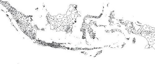
Figure 1 shows the administrative boundaries of 514 districts. The dots indicate the geographical centroids of those boundaries. In this map, the entire polygon structure of the administrative districts is not contiguous as water separates some islands. Given this lack of geographical contiguity, the queen contiguity criterion, which is the most commonly used approach to identify geographical neighbours, is not directly applicable. However, using the computational geometry approach described in Brassel and Reif (1979) and Aurenhammer (1991), one could take the centroids of the original administrative boundaries and derive a new polygon structure that is entirely contiguous. The use of this contiguous structure and its construction framework is described in the recent spatial analysis literature as the Thiessen polygon approach to generalised geographical contiguity (Anselin 2020).

FIGURE 1 Centroids of 514 Indonesian Districts and Associated Administrative Boundaries

Source: Authors.

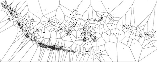
Figure 2 shows the 514 centroids of the Indonesian districts and their associated Thiessen polygon boundaries. The Thiessen polygons are formed by computing perpendicular bisectors between all neighbouring points. These polygons are suitable for identifying geographical neighbours based on their spatial contiguity. Thus, the neighbours of a district are those who share a common border or vertex in the Thiessen polygon structure.

FIGURE 2 Centroids of 514 Indonesian Districts and Associated Thiessen Polygon Boundaries

Source: Authors.

Some recent studies of Indonesia have used the Thiessen polygon approach to look at spatial inequality across districts and provinces. Santos-Marquez, Gunawan and Mendez (2021) used a Thiessen polygon structure to study the spatio-temporal dynamics of income per capita across 514 districts over 2010–17. Their results indicate that neighbour effects have played a significant role in slowing the pace of income convergence at the district level. Aginta, Miranti and Mendez (2021) also used a Thiessen polygon structure. They looked at regional growth and spatial dependence across Indonesian provinces during the Covid-19 pandemic. Their results indicate that negative spatial dependence during a pandemic is symptomatic of economic disintegration and lower economic growth. Overall, these recent studies suggest that a Thiessen polygon approach may be effective for modelling the spatial connectivity structure of Indonesia. Also, compared to the spatial distance perspective that has been used in previous studies (Vidyattama 2013, 2014), the Thiessen polygon approach provides a new and complementary perspective based on a generalised notion of geographical contiguity.

Exploratory Spatial Data Analysis

Several statistical tests have been used to evaluate the existence of spatial dependence in a data set. The most popular is Moran’s I test, which can be defined as the following:

where wij represents the spatial relationship between regions i and j (it is established from the structure defined in the earlier section on spatial connectivity structures); xi is the value of the variable x at location I; xj is the value of the same variable at location j; and µ is the cross-sectional mean of the data. Statistical inference for Moran’s I can be made using either an assumption of normality or a simulation of a reference distribution based on random permutations (Anselin 1995).

By recognising the specific location of spatial clusters and outliers, a local analysis of spatial autocorrelation complements the previously presented analysis of global dependence. Specifically, the local indicators of spatial association proposed by Anselin (1995) allow the identification of hot spots (high-value clusters), cold spots (low-value clusters) and spatial outliers (high values surrounded by low values and vice versa). The local version of Moran’s I test is computed for each spatial unit as follows:

where the notation follows that of equation 1. Statistical inference is based on a conditional permutation approach (Anselin 1995). One of the most appealing aspects of an analysis of local spatial dependence is the possibility of plotting statistically significant values on a map.

Regional Convergence and Spatial Models

Since the turn of the decade, the spatial econometric literature has revealed an increasing interest in the specification and estimation of econometric relationships using panel data sets. This interest is largely explained by the increasing availability of data sets that track the evolution of spatial units over time. Another advantage of panel data is that they enable researchers to conduct more advanced econometric modelling than the cross-sectional data that have been the focus of the spatial econometric literature since the late 1980s.

Islam (1995) first introduced a convergence framework for non-spatial panel data. His framework aimed to correct biases derived from unobserved heterogeneity and omitted variables. An early spatial panel data framework for convergence analysis was proposed by Arbia, Basile and Piras (2011). Specifically, they used a fixed-effect panel data model where spatial effects were modelled by involving spatially lagged covariates.

Elhorst (2010) summarised the relationships among spatial models and their spatial interaction effects. The most general spatial specification includes a spatially lagged dependent variable, spatially lagged independent variables and a spatially autocorrelated error term. In our paper, however, instead of using the most general (and complex) specification, we start our convergence analysis using the most basic non-spatial model: the standard linear regression model (SLM) estimated using the ordinary least squares (OLS) method. We begin with this model because it is simple and familiar to a large audience. While it is a non-spatial model, it is commonly used as a diagnostic tool and benchmark for comparisons with spatial models. The first spatial model we estimate is the spatial autoregressive (SAR) model. It indicates endogenous spatial interactions by way of a spatially lagged dependent variable. Using matrix notation, the SAR model is defined as follows:

where, in the context of this paper, y indicates the growth rate of HDI or GDP per capita, W is the spatial connective structure defined earlier, X is a matrix containing the explanatory variables (including the initial levels of HDI and GDP per capita), in is a vector of ones and ϵ is a random disturbance term.

Next, we estimate a spatial error model (SEM). This model indicates spatial interactions through the disturbance term. It is defined as follows:

The next model combines the spatial interactions of the two previously described models. Thus, it is usually referred to in the literature as the spatial autoregressive combined (SAC) model. The specification of this model is as follows:

Finally, we estimate a spatial Durbin model (SDM), which allows for spatial interactions in the dependent and independent variables. This model is specified as follows:

These four spatial specifications together with the non-spatial OLS model are used to evaluate Indonesia’s regional convergence process over 2000–2018. Three statistical frameworks have been proposed in the literature for estimating these spatial models. These are the maximum likelihood (ML) approach, the generalised method of moments (GMM) framework and the Bayesian Markov chain Monte Carlo approach.

From these estimation options, most of the literature on spatial convergence uses the ML approach.4 Arguably, a reason for this is that ML estimates are less biased and more efficient than GMM estimates when used with small data samples. A well-known limitation of the ML approach, however, is that it assumes that the errors of the regression model are normally distributed. Arbia, Le Gallo and Piras (2008) estimated spatial convergence models for the subnational regions of Europe using both ML and GMM methods. Their results suggest small differences between these two methods. Thus, to be consistent with most of the literature, we estimate spatial convergence models using the ML approach. Finally, to measure the goodness of fit of the non-spatial and spatial models, we use the Akaike information criterion (AIC) and Bayesian information criterion (BIC).

RESULTS

Exploratory Spatial Data Analysis

The evolution of regional disparities is depicted in figures 3a and 3b using the standard deviations of indicators for social development (HDI) and economic growth (GDP). The standard deviation values on the left Y-axis of each sub-figure indicate that disparities in HDI and GDP per capita have been decreasing over time.

FIGURE 3 Global Spatial Dependence and Sigma Convergence in Social and Economic Performance
Source: Authors.

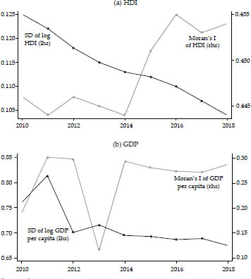
Both figures also present clear trends of global spatial autocorrelation. Global spatial autocorrelation is evaluated based on the value of Moran’s I indicator. The right Y-axes values of the figures indicate that the trend of spatial autocorrelation between 2010 and 2018 was increasing for both HDI and GDP. However, there was a sharp drop in Moran’s I indicator value for GDP in 2013. A noticeable implication of increasing spatial dependence is that regions have been performing more similarly over time. While regions grow, their performance suggests that they coordinate more with other close regions (Magalhães, Hewings and Azzoni 2005).

Furthermore, an appealing and important relationship is indicated by figures 3a and 3b: increasing patterns of spatial dependence tend to be associated with decreasing regional disparities, both in social (HDI) and economic (GDP) terms. Before delving deeper into that analysis, let us first discuss the local patterns of spatial dependence that aid in identifying regional clusters and potential spillovers.

The analysis of local indicators of spatial association proposed by Anselin (1995) is useful for identifying the location of spatial clusters and spatial outliers. Cold spots and hot spots are the spatial clusters in which spatial dependence is statistically significant. Cold spots are spatial clusters with significantly low values of HDI and GDP while hot spots are clusters with significantly high values. If there were a shock in any region of these clusters, a high degree of spatial dependence would facilitate the diffusion of the shock to neighbouring locations. Spatial outliers are defined as districts with significantly different performance levels from their neighbours.

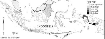
Figures 4–7 show the spatial distribution of regional development in terms of HDI and GDP per capita based on the location of spatial clusters and outliers. Hot spots (clusters of high values surrounded by other high values) are located in the western area of Indonesia, while cold spots (clusters of low values surrounded by other low values) are located in the eastern part of the country. Although social and economic disparities were decreasing during 2010–18, the east–west dichotomy was still present in 2018 (figures 5 and 7).

FIGURE 4 Local Indicators of Spatial Association of HDI in 2010

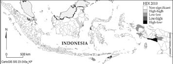
FIGURE 5 Local Indicators of Spatial Association of HDI in 2018

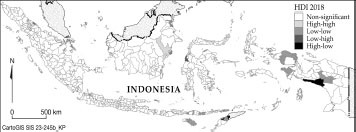
FIGURE 6 Local Indicators of Spatial Association of GDP Per Capita in 2010

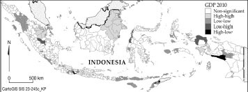
FIGURE 7 Local Indicators of Spatial Association of GDP Per Capita in 2018

In 2018, some districts did not show any changes in their human development level. Some districts in the eastern part of Indonesia (Papua and East Nusa Tenggara) were persistent in terms of their low social performance. In contrast, the number of low-performing districts in western parts of Indonesia (Tebing Tinggi City, South Jakarta and Penajam North Paser Regency) has decreased over time. Spatial outliers may also contribute to the reduction in regional disparities. It is worth highlighting that the numbers of spatial outliers were persistent in 2010 and 2018. Surprisingly, one district in Papua appears to have suffered negative spillovers from its neighbours. This district went from having highto low-level human development during 2010–18.

Concerning the local spatial dependence analysis of GDP per capita, the numbers of cold spots and hot spots are more pronounced. The hot spot clusters are comprised of districts rich in natural resources: East Kalimantan, Riau Islands, and some districts in Papua. Meanwhile, the cold spots are comprised of districts from North Sumatra, East Nusa Tenggara and the Maluku Islands. Spatial outliers are also detected in the spatial distribution of GDP per capita. Spatial outliers appear in Papua, the most vulnerable island. Spillovers appear to have large effects on this particular island.

Spatial Convergence Analysis for Panel Data

Few studies have implemented spatial convergence analyses in Indonesia. Furthermore, spatial panel data models are more complicated to estimate and interpret. In an attempt to obtain a precise estimation and select the most appropriate model, it is necessary to evaluate the role of spatial dependence and to control for unobserved regional heterogeneity. A spatial panel method is suitable for these tasks.

In this section, we show the results of our convergence analysis in five steps. First, we show that spatial dependence is a relevant phenomenon to be studied using panel data. For that purpose, we test the degree of cross-sectional dependence in the entire panel data set. Second, we show the results of an unconditional beta convergence model. That is, we show the relationship between the growth rate of HDI (or GDP) and its initial (log) level without control variables. If this relationship is negative and statistically significant, we can conclude that initially underdeveloped regions are catching up with more-developed regions. Third, we add control variables to the beta convergence model and study to what extent those variables affect the convergence speed of the regional system. In both of these steps, we focus on how spatial dependence affects the regional convergence speed. Fourth, we evaluate the robustness of our results using alternative spatial connective structures. Fifth, we decompose the total effect of each variable into its non-spatial and spatial components. The spatial component, also known as the indirect effect, is particularly interesting as it captures the direction and size of the spatial spillover effects.

Testing for Spatial Dependence in a Panel Data Setting

As shown, spatial dependence is statistically examined on a year-by-year basis. Also, spatial dependence can be simultaneously evaluated for all the years included in the analysis. For this more comprehensive approach, the literature typically employs Pesaran’s test for cross-sectional dependence. Table 2 shows that Pesaran’s test rejects the null hypothesis of cross-sectional independence. Thus, spatial panel data models may be more informative for studying the cross-sectional dynamics of HDI and GDP per capita.

Table 2. Pesaran’s Test of Cross-Sectional Dependence

Notes: The null hypothesis is cross-sectional independence. *** p < 0.01, ** p < 0.05, * p < 0.1

Spatial Dependence in the Unconditional Convergence Model

Tables 3 and 4 present the results of HDI and GDP per capita from the absolute convergence models for spatial dependence. Table 3 shows that the spatial Durbin model (SDM) is the best specification as it produces the lowest AIC and BIC index values. The inclusion of spatial dependence accelerates the catching-up period from more than 64 years to less than 13 years. The estimates from the spatial crossregressive parameters are also significant and positive, suggesting similarity in the performance of neighbouring regions.

Table 3. Spatial Dependence Results from the Absolute Convergence Models of HDI

Notes: Robust standard errors are in parentheses. The spatial connectivity structure (W, weight matrix) is based on the Thiessen polygon approach described earlier. Wg is the spatial lag of dependent variables; Wx is the spatial lag of independent variables.

*** p < 0.01, ** p < 0.05, * p < 0.1.

Table 4. Spatial Dependence Results from the Absolute Convergence Models of GDP Per Capita

Notes: Robust standard errors in parentheses. The spatial connectivity structure (W, weight matrix) is based on the Thiessen polygon approach described earlier. Wg is the spatial lag of the dependent variables; Wx is the spatial lag of the independent variables.

*** p < 0.01, ** p < 0.05, * p < 0.1.

Table 4 shows a similar tendency in terms of the convergence parameter estimates and the best choice of model. Based on table 4, the SDM appears to be the best specification with the lowest AIC and BIC values. In terms of the convergence indicators, almost 14 years are needed to halve the disparities in GDP per capita. The inclusion of spatial dependence accelerates the catching-up period from more than 35 years to just under 14 years. The spatial cross-regressive parameter values are also significant and positive.

Spatial Dependence in the Conditional Convergence Model

This section discusses the findings of conditional convergence. Tables 5 and 6 provide the results from the conditional convergence framework for both HDI and GDP per capita. This study contains a rich data set of various characteristics across districts. Thus, the conditional convergence framework is applied to give a more complete description of the structural characteristics of the districts. Three well-known predictors widely used in growth studies are evaluated. They are human capital, economic structures (agriculture, industry and services) and investment share.

Table 5. Spatial Dependence in the Conditional Convergence Models of HDI and Determinants

Notes: Robust standard errors in parentheses. The spatial connectivity structure (weight matrix, W) is based on the Thiessen polygon approach described earlier. Wg is the spatial lag of dependent variables; Wx is the spatial lag of independent variables.

*** p < 0.01, ** p < 0.05, * p < 0.1

Table 6. Spatial Dependence in the Conditional Convergence Models of GDP per capita and Determinants

Notes: Robust standard errors are in parentheses. The spatial connectivity structure (weight matrix, W) is based on the Thiessen polygon approach described earlier. Wg and Wx represent the spatial lags of the relevant variables. W error (spatial error ) represents the error terms across different spatial units.

*** p < 0.01, ** p < 0.05, * p < 0.1.

Table 5 presents the spatial dependence results from the conditional convergence model for HDI. The best specification, because it has the lowest AIC and BIC values, is the SDM. Table 5 shows that, while some of the newly added variables are statistically significant, they have a limited effect on the regional convergence speed. Furthermore, the spatial lag of initial HDI (SLM) is also statistically significant and positive. This implies that a given district’s HDI tends to grow faster if the initial levels of HDI in the neighbouring districts are high. In particular, the share of the industry sector and the share of the services sector significantly affect human development convergence in a given district, although the magnitude of the effect is small. Moreover, the spatial lags of the log of initial HDI, share of agriculture and share of services sector are noteworthy for their statistical significance. Thus, on average, changes in those variables in a district will influence the growth of human development in neighbouring districts.

Table 6 describes the role of spatial dependence in the conditional convergence model for GDP per capita. The best specification is also the SDM since it has the smallest AIC and BIC values. Table 6 shows that none of the newly added conditional variables of GDP per capita growth is statistically significant. However, the spatial lag of initial GDP (SLM) per capita remains statistically significant and positive. This implies that a higher initial level of GDP per capita in a given district tends to increase the growth of GDP per capita in the neighbouring districts. Based on the findings, although HDI and GDP per capita capture different phenomena, their convergence stories are consistent: initially poor districts are catching up with more-developed districts and spatial dependence accelerates this process.

Robustness to Alternative Connectivity Structures

With SDM as the benchmark, we compare the estimation of each variable and convergence indicator using two different spatial connectivity structures (weight matrices W1 and W2). In this paper, the contiguity-based Thiessen polygon (W1) is the main (baseline) structure and the inverse distance matrix (W2) is the alternative. Table 7 compares the results of the two connectivity structures (W1 and W2).

Table 7. Comparison of Spatial Durbin Model Using Two Different Weight Matrices

Notes: Robust standard errors are in parentheses. W1 is a contiguity-based Thiessen polygon matrix; W2 is an inverse distance matrix.

*** p < 0.01, ** p < 0.05, * p < 0.1.

In terms of the convergence speeds and half-lives for HDI, both connectivity structures produce similar results. For growth in GDP per capita, however, the convergence speeds are fractionally faster and the half-lives are slightly shorter when the inverse distance criteria are used (W2). For HDI, when using a contiguitybased Thiessen polygon (W1), the coefficient of spatial cross-regression indicates that there is a positive and significant association between the HDI growth in a district and its surrounding neighbourhood. In contrast, when using an inverse distance matrix, there is an insignificant and negative association between the growth of HDI in a district and its surrounding neighbourhood. However, both connectivity structures produce negative spatial coefficients for growth in GDP per capita. Those coefficients mean that an increase in a district’s economic size could lower the surrounding districts’ economic performance. This surprising finding could serve as a warning for policymakers to further develop supportive inter-regional policies that allow regions to grow at similar rates.

Direct and Indirect Effects

Many empirical studies have used the coefficient estimates of one or more spatial regressions to conclude whether or not spatial spillovers exist. In a spatial econometric model, if the SDM is adopted, both the direct and indirect effects of a particular explanatory variable will depend on the coefficient estimate of the spatially lagged value of that variable. The result is that no prior restriction is placed on the magnitude of both direct and indirect effects. Thus, the ratio between indirect and direct effects may be different for different explanatory variables. Because of this flexibility, the SDM is a more attractive starting point for an empirical study than other spatial regression specifications.

Table 8 shows the direct and indirect effects of key variables on HDI and GDP per capita under the SDM. The more relevant of these two effect types is the indirect effect because the coefficient estimate indicates the direction and size of the spatial spillover. The indirect effect of the log of initial HDI is positive. This suggests that when poor regions are surrounded by other poor regions, the convergence slows owing to the overall poorness of the neighbourhood. This convergence-reducing spillover effect is also present in the case of GDP per capita. The practical implication is that when an initially low-income district is surrounded by other low-income districts, the low income of its neighbours tends to lessen its convergence prospects.

Table 8. Direct and Indirect Effects of Key Variables on HDI and GDP per capita under the Spatial Durbin Model

Notes: Robust standard errors are in parentheses. W1 is a contiguity-based Thiessen polygon matrix; W2 is an inverse distance matrix.

*** p < 0.01, ** p < 0.05, * p < 0.1.

In terms of the direct effect of structural variables (share of agriculture, share of industry and share of services sector ), only the share of the industry sector has a positive coefficient, which suggests a positive relationship between increases in that sector’s share and increases in the growth rate of HDI. Thus, the development of the industry sector, especially in underdeveloped districts, could help to increase HDI. The lack of statistical significance in the coefficient for the share of the agriculture sector indicates that further research is needed to evaluate the role of agriculture in the regional convergence process.

The coefficient for the mean years of schooling is negative while that for the expected years of schooling is positive. However, neither of these proxies of human capital has a statistically significant effect on GDP per capita. The (indirect) spillover effect of the mean years of schooling in a district is positive and statistically significant. This means that a higher average period of schooling in a region tends to increase the rate of GDP growth in neighbouring districts. However, an increase in the expected years of schooling in one district would decrease the rate of GDP growth in the surrounding districts. This last result is counter-intuitive and deserves further investigation.

DISCUSSION

The main purpose of this article is to assess regional convergence dynamics from social and economic standpoints. To do that, we have used both non-spatial and spatial convergence frameworks. Additionally, we have taken into account the significant social and economic inequalities between districts by adding control variables in our spatial convergence models.

Using a cross-sectional convergence framework, Miranti and Mendez-Guerra (2020) found regional convergence in HDI and its components. She also found that small differences between the speeds of spatial and non-spatial types of convergence have large implications in terms of the years that are needed to reduce regional disparities. The results from the spatial regressions (tables 3 and 4) suggest that spatial effects are significant in accelerating the catching-up process of districts in terms of their human development and economic outcomes. When we included spatial effects in our convergence models, we found that the time required to halve disparity is shorter. In particular, it would take about 12–13 years to halve inequality in human development in a district. Meanwhile, it would take about 13–14 years to halve economic disparity.

Among all the control variables, the effects of the initial level of human development and economic-related variables are statistically significant in determining a given year’s growth in human development. Also, while an increasing share of the services sector is associated with a reduction in the growth rate of human development, the regression coefficient for this relationship is close to zero. In the economic convergence model, the initial economic size of each region helps the region grow economically in a given year.

Owing to the presence of direct and indirect effects, the spatial convergence framework is more informative than the classical convergence model. The direct effect of the initial human development is the average change in a district’s human development growth due to a one-unit change in that district’s initial level. The indirect effect, conversely, can be defined as the aggregate effect of a change in a variable in neighbouring districts on the growth rate of a particular district.As argued by Le Sage and Pace (2009), the indirect effect indicates the contribution of spatial spillovers. Initial human development and initial GDP per capita have a positive indirect effect on GDP and HDI growth, implying that the benefits of having high initial levels of human development or GDP in a district would spread to neighbouring districts.

CONCLUDING REMARKS

Sustainable development occurs when economic progress is coupled with social inclusion. To understand sustainable development at the subnational level in Indonesia, we studied regional convergence dynamics based on two indicators: HDI and GDP per capita. Our sample covers 514 districts over 2010–18. The main result of the analysis indicates that a process of regional convergence is occurring and spatial dependence across districts plays an important role in this process. Furthermore, the convergence speed of HDI is slightly faster than that of GDP per capita.

Results from a global spatial autocorrelation analysis indicate positive spatial dependence in both HDI and GDP per capita. Moreover, over time, increasing spatial dependence is negatively associated with decreasing regional inequality. This result suggests that spatial interactions can play an essential role in the reduction of regional inequality by helping the poorest districts catch up with wealthier districts faster. Results from a local spatial autocorrelation analysis indicate larger and more numerous spatial clusters in the case of HDI compared with GDP per capita.

Results from various panel data regressions indicate that spatial models provide a better characterisation of the regional convergence process of Indonesia. In particular, a spatial Durbin specification provides the best fit and accommodates spatial dependence in regional growth rates as well as their determinants. These results are robust to alternative spatial connectivity structures. Among the determinants of social convergence, the share of industry and the share of services sectors show statistically significant effects, although they work in opposite directions. Overall, sectoral components of the economy must be considered to help regions that are lagging both socially and economically to catch up with better-off regions.

The standard neoclassical convergence framework and its spatial dependence extension, as used in this paper, assume convergence towards a single long-run equilibrium. This type of analysis is commonly used in the convergence literature as a first approximation for understanding regional dynamics. Nevertheless, this analysis abstracts from the role of regional heterogeneity and multiple equilibria, which are reported to be key features of the Indonesian economy (Kurniawan, de Groot and Mulder 2019; Mendez and Kataoka 2021; Aginta, Miranti and Mendez 2021). Further research is needed in this area. In particular, two extensions appear promising. First, using district-level data, multiple equilibria could be identified based on the convergence framework of Phillips and Sul (2007), and the determinants of the convergence clubs could be evaluated using an ordered logit model as done by Gunawan, Mendez and Otsubo (2021). Second, spatial heterogeneity could be modelled using the new multiscale, geographically weighted regression model of Fotheringham, Yang and Kang (2017). As shown in other studies, these extensions provide a more nuanced view of the regional convergence process. However, the analytical complexity of such nuances is usually better understood if contextualised with an intuitive and parsimonious benchmark, which we aimed to introduce in this paper.

Notes

1 A neighbourhood effect, or spatial spillover effect, can be understood as the effect or change in an area, either positively or negatively, due to a change in an area that shares a border.

2 Given the archipelago configuration of Indonesia, a spatial connectivity structure based on geographical contiguity cannot be directly constructed. Contiguity is indirectly measured based on an estimated Thiessen polygon.

3 Although the main spatial connectivity structure used in this paper is based on the Thiessen polygon, we also use an inverse distance approach for robustness and comparison purposes.

4 See, for instance, Rey and Montouri (1999), Arbia, Le Gallo and Piras (2008) and Panzera and Postiglione (2021).

REFERENCES

- Aginta, Harry, Ragdad C. Miranti and Carlos Mendez. 2021. ‘Regional Economic Growth Convergence and Spatial Growth Spillovers at Times of Covid-19 Pandemic in Indoneia’. In Regional Perspectives of Covid-19 in Indonesia, edited by Budy P. Resosudarmo, Tri Mulyaningsih, Dominicus S. Priyarsono, Devanto Pratomo and Arief A. Yusuf, 31–54. IRSA Press, Yogyakarta.
- Akita, Takahiro. 1988. ‘Regional Development and Income Disparities in Indonesia’. Asian Economic Journal 2 (2): 165–91. https://doi.org/10.1111/j.1467-8381.1988.tb00131.x
- Akita, Takahiro. 2002. ‘Regional Income Inequality in Indonesia and the Initial Impact of the Crisis’. Bulletin of Indonesian Economic Studies 38 (2): 201–22. https://doi.org/10.1080/000749102320145057
- Akita, Takahiro and Rizal A. Lukman. 1995. ‘Interregional Inequalities in Indonesia: A Sectoral Decomposition Analysis for 1975–92’. Bulletin of Indonesian Economic Studies 31 (2): 61–81 https://doi.org/10.1080/00074919512331336785
- Anselin, Luc. 1995. ‘Local Indicators of Spatial Association—LISA’. Geographical Analysis 27 (2): 93– 115. doi: 10.1111/j.1538-4632.1995.tb00338.x
- Anselin, Luc. 2020. ‘Distance-Band Spatial Weights’. GeoDa: An Introduction to Spatial Data Science. Last modified 10 August 2020. https://geodacenter.github.io/workbook/4b_dist_weights/lab4b.html#:~:text=serves%20our%20purposes.-,Distance%2Dband%20weights,critical%20distance%20band%20from%20i.
- Arbia, Giuseppe, Roberto Basile and Mirella Salvatore. 2003. ‘Measuring Spatial Effects in Parametric and Nonparametric Modelling of Regional Growth and Convergence’. Paper presented at the project meeting of the United Nations University and World Economic Institute for Development Research on spatial inequality in development, Helsinki, May 2003.
- Arbia, Giuseppe, Julie Le Gallo and Gianfranco Piras. 2008. ‘Does Evidence on Regional Economic Convergence Depend on the Estimation Strategy? Outcomes from Analysis of a Set of NUTS2 EU Regions’. Spatial Economic Analysis 3 (2): 209–24. doi: 10.1080/17421770801996664
- Arbia, Giuseppe, Roberto Basile and Gianfranco Piras. 2011. ‘Using Spatial Panel Data in Modelling Regional Growth and Convergence’. Working paper, Institute for Studies and Economic Analyses, Rome, September 2011.
- Artis, Michael J. and Dilip Nachane. 1990. ‘Wages and Prices in Europe: A Test of the German Leadership Thesis. Weltwirtschaftliches Archiv 126 (1): 59–77. https://www.jstor.org/stable/40439766 doi: 10.1007/BF02706312
- Aurenhammer, Franz. 1991. ‘Voronoi Diagrams—A Survey of a Fundamental Geometric Data Structure’. ACM Computing Surveys 23 (3): 345–405. doi: 10.1145/116873.116880
- Barro, Roberto J. and Xavier Sala-i-Martin. 1991. ‘Convergence across States and Regions’. Brookings Papers on Economic Activity (1): 107–82. https://doi.org/10.2307/2534639
- Barro, Roberto J. and Xavier Sala-i-Martin. 1992. ‘Convergence’. Journal of Political Economy 100 (2): 223–51. doi: 10.1086/261816
- Baumol, William J. 1986. ‘Productivity Growth, Convergence, and Welfare: What the Long-Run Data Show’. American Economic Review 76 (5): 1072–85.
- Beine, Michel, Frédéric Docquier and Alain Hecq. 1999. ‘Convergence des Groupes en Europe: Une Analyse sur Données Régionales’ [Convergence of Groups in Europe: An Analysis of Regional Data]. Universite Libre de Bruxelles Institutional Repository 2013/10459. https://ideas.repec.org/p/ulb/ulbeco/2013-10459.html
- Bernard, Andrew B. and Steven N. Durlauf. 1995. ‘Convergence in International Output’. Journal of Applied Econometrics 10 (2): 97–108. https://doi.org/10.1002/jae.3950100202
- Bernat, Andrew G., Jr. 1996. ‘Does Manufacturing Matter? A Spatial Econometric View of Kaldor’s Laws’. Journal of Regional Science 36 (3): 463–77. https://doi.org/10.1111/j.1467-9787.1996.tb01112.x
- Bianchi, Marco. 1997. ‘Testing for Convergence: Evidence from Non-parametric Multimodality Tests’. Journal of Applied Econometrics 12 (4): 393–409. https://doi.org/10.1002/(SICI)1099-1255(199707)12:4<393::AID-JAE447>3.0.CO;2-J
- Brassel, Kurt E. and Douglas Reif. 1979. ‘A Procedure to Generate Thiessen Polygons’. Geographical Analysis 11(3): 289–303. doi: 10.1111/j.1538-4632.1979.tb00695.x
- Canova, Fabio and Albert Marcet. 1995. ‘The Poor Stay Poor: Non-convergence across Countries and Regions’. CEPR Press Discussion Paper 1265. https://cepr.org/publications/dp1265
- Day, Jennifer and Peter Ellis. 2014. ‘Urbanization for Everyone: Benefits of Urbanization in Indonesia’s Rural Regions’. Journal of Urban Planning and Development 140 (3): 04014006.https://doi.org/10.1061/(ASCE)UP.1943-5444.0000164
- Day, Jennifer and Blane Lewis. 2013. ‘Beyond Univariate Measurement of Spatial Autocorrelation: Disaggregated Spillover Effects for Indonesia’. Annals of GIS 19 (3): 169–85. https://doi.org/10.1080/19475683.2013.806353
- Desdoigts, Alain. 1999. ‘Patterns of Economic Development and the Formation of Clubs’. Journal of Economic Growth 4 (3): 305–30. https://doi.org/10.1023/A:1009858603947
- Elhorst, J. Paul. 2010. ‘Applied Spatial Econometrics: Raising the Bar’. Spatial Economic Analysis 5 (1): 9–28. https://doi.org/10.1080/17421770903541772
- Esmara, Hendra. 1975. ‘Regional Income Disparities’. Bulletin of Indonesian Economic Studies 11 (1): 41–57. https://doi.org/10.1080/00074917512331332622
- Fotheringham, A. Stewart, Wenbai Yang and Wei Kang. 2017. ‘Multiscale Geographically Weighted Regression (MGWR)’. Annals of the American Association of Geographers 107 (6): 1247–65. https://doi.org/10.1080/24694452.2017.1352480
- Garcia, Jorge G. and Lana Soelistianingsih. 1998. ‘Why Do Differences in Provincial Incomes Persist in Indonesia?’ Bulletin of Indonesian Economic Studies 34 (1): 95–120. https://doi.org/10.1080/00074919812331337290
- Gunawan, Anang B., Carlos Mendez and Shigeru Otsubo. 2021. ‘Provincial Income Conver-gence Clubs in Indonesia: Identification and Conditioning Factors’. Growth and Change 52 (4): 2540–75. https://doi.org/10.1111/grow.12553
- Hill, Hal, Budy Resosudarmo and Yogi Vidyattama. 2008. ‘Indonesia’s Changing Economic Geography’. Bulletin of Indonesian Economic Studies 44 (3): 407–35. https://doi.org/10.1080/00074910802395344
- Islam, Nazrul. 1995. ‘Growth Empirics: A Panel Data Approach’. Quarterly Journal of Economics 110 (4): 1127–70. doi: 10.2307/2946651
- Kataoka, Mitsuhiko. 2019. ‘Interprovincial Differences in Labour Force Distribution and Utilization based on Educational Attainment in Indonesia, 2002–2015’. Regional Science Policy & Practice 11 (1): 39– 54. doi: 10.1111/rsp3.12159
- Kosfeld, Reinhold, Hans-Friedrich Eckey and Christian Dreger. 2005. ‘Regional Convergence in Unified Germany: A Spatial Econometric Perspective’. In Advances in Macroeconometric Modeling, Papers and Proceedings of the 4th IWH Workshop in Macroeconometrics, edited by Christian Dreger and Gerd Hansen, 79–111. Baden-Baden: Nomos Publishers.
- Kurniawan, Hengky, Henry L.F de Groot and Peter Mulder. 2019. ‘Are Poor Provinces Catch-ing-up the Rich Provinces in Indonesia?’ Regional Science Policy & Practice 11(1): 89–108 doi: 10.1111/rsp3.12160
- Le Sage, James and R. Kelley Pace. 2009. Introduction to Spatial Econometrics. Boca Raton: Chapman & Hall.
- Magalhães, André, Geoffrey J. D. Hewings and Carlos R. Azzoni. 2005. ‘Spatial Dependence and Regional Convergence in Brazil’. Journal of Regional Research (6): 5–20.
- Mankiw, N. Gregory, David Romer and David N. Weil. 1992. ‘A Contribution to the Empirics of Economic Growth’. Quarterly Journal of Economics 107 (2): 407–37. doi: 10.2307/2118477
- McCulloch, Neil and Bambang S. Sjahrir. 2008. ‘Endowments, Location or Luck? Evaluating the Determinants of Sub-national Growth in Decentralized Indonesia.’ Policy Research Working Paper 4769, World Bank, Washington, DC.
- Mello, Marcelo. 2010. ‘Stochastic Convergence across U.S. States’. Macroeconomic Dynamics 15 (2): 160–83. doi: 10.1017/S1365100509991106
- Mendez, Carlos. 2020. ‘Regional Efficiency Convergence and Efficiency Clusters: Evidence from the Provinces of Indonesia 1990–2010’. Asia-Pacific Journal of Regional Science (4): 391–411. https://doi.org/10.1007/s41685-020-00144-w
- Mendez, Carlos and Mitsuhiko Kataoka. 2021. ‘Disparities in Regional Productivity, Capital Accumulation, and Efficiency across Indonesia: A Club Convergence Approach’. Review of Development Economics 25 (2): 790–809. doi: 10.1111/rode.12726
- Milanovic, Branko. 2005. ‘Half a World: Regional Inequality in Five Great Federations’. Journal of the Asia Pacific Economy 10 (4):408–45. https://doi.org/10.1080/13547860500291562
- Miranti, Ragdad Cani. 2021. ‘Is Regional Poverty Converging across Indonesian Districts? A Distribution Dynamics and Spatial Econometric Approach’. Asia-Pacific Journal of Regional Science 5:851–83. https://doi.org/10.1007/s41685-021-00199-3
- Miranti, Ragdad Cani and Carlos Mendez-Guerra. 2020. ‘Human Development Disparities and Convergence across Districts of Indonesia: A Spatial Econometric Approach’. IDEAS Working Paper Series, RePEc.
- Niebuhr, Annekatrin. 2000. ‘Convergence and the Effects of Spatial Interaction’. HWWA Discussion Paper 110, Hamburg Institute of International Economics, March. https://econpapers.repec.org/RePEc:zbw:hwwadp:26351
- Panzera, Domenica and Paolo Postiglione. 2021. ‘The Impact of Regional Inequality on Economic Growth: A Spatial Econometric Approach’. Regional Studies 56 (5): 687–702. doi: 10.1080/00343404.2021.1910228
- Phillips, Peter C. and Donggyu Sul. 2007. ‘Transition Modeling and Econometric Convergence Tests’. Econometrica 75 (6): 1771–855. doi: 10.1111/j.1468-0262.2007.00811.x
- Quah, Danny T. 1997. ‘Empirics for Growth and Distribution: Stratification, Polarization, and Convergence Clubs’. Journal of Economic Growth 2 (1): 27–59. doi: 10.1023/A:1009781613339
- Resosudarmo, Budy P. and Yogi Vidyattama. 2006. ‘Regional Income Disparity in Indonesia: A Panel Data Analysis’. ASEAN Economic Bulletin 23 (1): 31–44. https://www.jstor.org/ stable/41316942 doi: 10.1355/AE23-1C
- Rey, Sergio J. and Brett D. Montouri. 1999. ‘US Regional Income Convergence: A Spatial Econometric Perspective’. Regional Studies 33 (2): 143–56. https://doi.org/10.1080/00343409950122945
- Rumayya, Wirya Wardaya and Erlangga Agustino Landiyanto. 2005. ‘Club Convergence & Regional Spillovers in East Java’. Paper presented at Parallel Session VB: Regional Economic Development, Jakarta, November. https://econwpa.ub.uni-muenchen.de/econ-wp/ge/papers/0511/0511008.pdf
- Santos-Marquez, Felipe, Anang Gunawan and Carlos Mendez. 2021. ‘Regional Income Disparities, Distributional Convergence, and Spatial Effects: Evidence from Indonesian Regions 2010–2017’. GeoJournal 87: 2373–91. https://doi.org/10.1007/s10708-021-10377-7
- Solow, Robert M. 1956. ‘A Contribution to the Theory of Economic Growth’. Quarterly Journal of Economics 70 (1): 65–94. doi: 10.2307/1884513
- Tadjoeddin, Mohammad Z., Widjajanti I. Suharyo and Satish Mishra. 2001. ‘Regional Disparity and Vertical Conflict in Indonesia’. Journal of the Asia Pacific Economy 6 (3): 283–304. https://doi.org/10.1080/13547860120097368
- Uppal, J.S. and Budiono Sri Handoko. 1986. ‘Regional Income Disparities in Indonesia’. EKI 34 (3): 287–304.
- Vidyattama, Yogi. 2006. ‘Regional Convergence and Indonesia Economic Dynamics’. Economics and Finance in Indonesia 54 (2): 197–227. https://www.lpem.org/repec/lpe/efijnl/200608.pdf doi: 10.7454/efi.v54i2.97
- Vidyattama, Yogi. 2013. ‘Regional Convergence and the Role of the Neighbourhood Effect in Decentralised Indonesia’. Bulletin of Indonesian Economic Studies 49 (2): 193–211. https://doi.org/10.1080/00074918.2013.809841
- Vidyattama, Yogi. 2014. ‘Issues in Applying Spatial Autocorrelation on Indonesia’s Provincial Income Growth Analysis’. Australasian Journal of Regional Studies 20 (2): 375–402.