Computing Data-driven Multilinear Metro Maps

ABSTRACT

Traditionally, most schematic metro maps in practice as well as metro map layout algorithms adhere to an octolinear layout style with all paths composed of horizontal, vertical, and ${45}^{\circ }$-diagonal edges. Despite growing interest in more general multilinear metro maps, generic algorithms to draw metro maps based on a system of $k\ge 2$ not necessarily equidistant slopes have not been investigated thoroughly. In this paper, we present and implement an adaptation of the octolinear mixed-integer linear programming approach of Nöllenburg and Wolff (2011) that can draw metro maps schematized to any set $\mathcal{C}$ of arbitrary orientations. We further present a data-driven approach to determine a suitable set $\mathcal{C}$ by either detecting the best rotation of an equidistant orientation system or by clustering the input edge orientations using a k-medians algorithm. We demonstrate the new possibilities of our method using several real-world examples.

KEYWORDS:

• Metro map layout
• $\mathcal{C}$-oriented schematization
• mixed integer linear programming

Introduction

Metro maps are ubiquitous schematic network diagrams that aid public transit passengers in orientation and route planning in almost all types of urban public transit systems worldwide. Since Henry Beck's classic schematic London Tube Map of 1933, metro maps have developed a common visual language and adopted similar design principles (Wu et al., 2020). Designing professional metro maps is still mostly a manual task today, even if cartographers and graphic designers are supported by digital drawing tools. Algorithms for automated layout of metro maps have received substantial interest in the graph drawing and network visualization communities as well as in cartography and geovisualization over the last 20 years (Wolff, 2007; Nöllenburg, 2014; Wu et al., 2020). The vast majority of metro map layout algorithms focus on so-called octolinear (sometimes also called octilinear) metro maps which are limited to Henry Beck's classical and since then widely adopted ${45}^{\circ }$-angular grid of line orientations (Garland, 1994). However, not all metro maps found in practice are strictly octolinear. In fact, there does not seem to be a one-size-fits-all layout for every network.

There is empirical evidence from usability studies that the best set of line orientations for drawing a metro map depends on different aspects of the respective transit network, and it may not always be an octolinear one (Roberts et al., 2013, 2017). A chain of recent publications (Niedermann et al., 2019; Niedermann and Rutter, 2020; Barth et al., 2021) developed a Topology-Shape-Metrics Framework for orthoradial graph drawing. In this style, all edges are either arcs of concentric circles or straight-line segments of lines through the centre of the circles. Orthoradial drawings of metro maps have received come attention outside of scientific research, e.g. through the change in the official metro map of Cologne, Germany to an orthoradial map (KVB, 2022). Another framework which is capable of computing ortho-radial maps is the octi-framework (Bast et al., 2020, 2021) which uses repeated (or simultaneous) shortest path computation on a predefined grid. This discretization enables alternative layouts; however, it is restricted to those that are easily expressible as a regular grid.

In this paper, we present an algorithmic approach using global optimization for computing (unlabeled) metro maps in the more flexible k-linearity setting, where each edge in the drawing must be parallel to one of $k\ge 2$ equidistant orientations whose pairwise angles are multiples of ${360}^{\circ }/2k$. In this sense, a k-linear map for k = 4 corresponds to the traditional octolinear setting. In fact, most octolinear maps use a horizontally aligned orientation system, i.e. a system that includes a horizontal orientation. It is possible though, for some transit networks and city geometries, that a rotation of the orientation system by an angular offset yields a more topographically accurate metro map layout. Hence we also consider such rotated k-linear maps. In addition to equiangular k-linear orientation systems, we further study irregular multilinear (or $\mathcal{C}$-oriented) maps (Roberts et al., 2017), in which the edges are parallel to any given, not necessarily equiangular set $\mathcal{C}$ of orientations. There exist a number of metro map layout algorithms (see Nöllenburg, 2014; Wu et al., 2019, 2020 for comprehensive surveys) that would technically permit an adaptation to a different underlying angular grid, yet most previous papers optimize layouts in the well-known octolinear setting only and do not discuss extensions to different linearities. A few algorithms for generic multilinear or k-linear layouts exist (Neyer, 1999; Merrick and Gudmundsson, 2007; Delling et al., 2014; Buchin et al., 2016), but they are aimed at paths or polygons rather than entire metro maps. In the field of graph drawing many algorithms for planar orthogonal network layouts with k = 2 as well as for polyline drawings with completely unrestricted slopes are known (Duncan and Goodrich, 2013), but they do not generalize to k-linearity and multilinearity.

Contributions. We first present two efficient approaches for deriving suitable, data-dependent linearity systems (rotated k-linear and irregular multilinear) by minimizing the angular distortion of the input edge slopes (Section ‘Orientation Systems’). We then adapt an existing octolinear mixed-integer linear programming (MIP) model (Nöllenburg and Wolff, 2011) by generalizing their mathematical layout constraints to k-linearity and multilinearity (Section ‘MIP Model’). The main benefit of this model in comparison to other approaches is that it defines sets of hard and soft constraints and guarantees that the computed layout satisfies all the hard constraints, while the soft constraints are globally optimized. The trade-off for providing such quality guarantees from a global optimization technique is that computation time is typically higher compared to other methods (Wu et al., 2019). By modeling fundamental metro map properties such as strict adherence to the given linearity system and topological correctness as hard constraints, we obtain layouts that satisfy these layout requirements strictly. The soft constraints optimize for line straightness, compactness, and topographicity (Roberts, 2014), i.e. low topographical distortion. Our modifications yield a flexible MIP model, whose complexity measured by the number of variables and constraints grows linearly with the number of orientations k. We finally demonstrate the effect of horizontally aligned and rotated k-linear and multilinear orientation systems by providing sample layouts of six metro networks and evaluating the resulting number of bends and angular distortions for typical small values of k = 3, 4 and 5 (Section ‘Experiments’).

Preliminaries

We reuse previously established notation (Nöllenburg and Wolff, 2011). The input is represented as an embedded planar metro graph $G=(V,E)$ with n vertices and m edges. For non-planar metro graphs we temporarily introduce a dummy vertex for each edge crossing which preserves the crossing in the output layout. Each vertex $v\in V$ represents a metro station with x- and y-coordinates and each edge $e=(u,v)\in E$ is a segment linking vertices u and v that represents a physical rail connection between them. Let $\mathcal{L}$ be a line cover of G, i.e. a set of paths in G such that each edge $e\in E$ belongs to at least one path $L\in \mathcal{L}$. An element $L\in \mathcal{L}$ is called a line and corresponds to a metro line in the underlying transit network. Note that multiple lines can pass through the same edge. Finally, $k\ge 2$ is an input parameter that defines the number of available edge orientations in the orientation system $\mathcal{C}$. 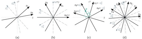The set $\mathcal{C}$ and the parameter k can be part of the input or they can be derived automatically from the input graph, see Section ‘Orientation Systems’. Figure 1 shows some examples of orientation systems. Since every orientation can be used in two directions this yields $2k$ available drawing directions. Let $\mathcal{K}$ be this set of $2k$ directions. We note that every edge is assigned exclusively to an outgoing direction of its incident vertices, which implies that the maximum degree of G can be at most $2k$. Thus the maximum degree in G provides a lower bound on the required number of orientations. Note that high-degree vertices can be handled in different ways, like splitting them into lower-degree dummy vertices. The result would be a graph with lower maximum degree, which in turn could be used as input for our problem.

Figure 1. Coordinate axes for different orientation systems. (c) illustrates a point p with the redundant coordinates $p=(0,1,\sqrt{2},1)$. (a) k = 2, irregular. (b) k = 3, regular aligned. (c) k = 4, regular rotated and (d) k = 5, regular rotated.

The general algorithmic metro map layout problem studied in this paper is to find a $\mathcal{C}$-oriented schematic layout of $(G,\mathcal{L})$, i.e. a graph layout that preserves the input topology, uses only edge directions parallel to an orientation from $\mathcal{C}$, and optimizes a weighted layout quality function (here composed of line straightness, topographicity, and compactness). If $\mathcal{C}$ corresponds to a k-linear orientation system, we also call the layout k-linear instead of $\mathcal{C}$-oriented; otherwise, it can alternatively be called multilinear.

Orientation Systems

A set of edge orientations (or an orientation system) $\mathcal{C}=\{c_1,\dots ,c_k\}$ is a set of k angles (expressed in radian), where $0\le c_1<\cdots <c_k<\pi$. We distinguish three different kinds of possible edge orientation sets. An edge orientation set $\mathcal{C}$ is called regular (or equiangular) if the angles $\{c_1,\dots c_k\}$ divide the range $[c_1,c_1+\pi )$ into k parts of equal size $\pi /k$, i.e. $c_i-c_{i-1}=\pi /k$ for all $i\in \{2,\dots ,k\}$. Otherwise, we call $\mathcal{C}$ irregular. The special case of a regular orientation system $\mathcal{C}$, in which $c_1=0$ is called aligned. Note that a classical octolinear layout is based on the aligned orientation system ${\mathcal{C}}_o=\{0,\pi /4,\pi /2,3\pi /4\}$.

Opposed to an aligned orientation system, which is fully specified by defining the number k of orientations, we have more degree of freedom in a regular (non-aligned) and an irregular system. The next two sections describe how to derive a suitable system $\mathcal{C}$ from the geometric properties of the input data. The idea behind this approach is to better minimize the topographic distortion of the schematized edges compared to their input direction.

We measure the distortion ${\mathrm{dist}}_G\left(\mathcal{C}\right)$ of a system $\mathcal{C}$ with respect to a metro graph G by summing up the difference in slope between each edge $e\in E$ (with slope ${\gamma }_e$) and the angle $c\in \mathcal{C}$ which is closest to ${\gamma }_e\mathrm{mod}\pi$. Note that since we are only interested in the smaller of the two angles and the range of c and ${\gamma }_e\mathrm{mod}\pi$ is $[0,\pi )$, we define the ‘distance’ $d(c,{\gamma }_e)$ between c and ${\gamma }_e$ as $d(c,{\gamma }_e)=min\left(\right|c-\left({\gamma }_e\mathrm{mod}\pi \right)|,\pi -|c-\left({\gamma }_e\mathrm{mod}\pi \right)\left|\right)$. Then the distortion of $\mathcal{C}$ with respect to G is computed as: ${\mathrm{dist}}_G\left(\mathcal{C}\right)=\sum _{e\in E}\left(\underset{c\in \mathcal{C}}{min}d\right(c,{\gamma }_e\left)\right).$Note that in a schematization of G every edge can use an orientation $c\in \mathcal{C}$ in both directions, i.e. there is a large difference between drawing an edge in one direction corresponding to orientation c and drawing it with the opposite direction (which still has orientation c). To account for this we have to measure the actual distortion of a schematization differently. For every orientation c, let $\overline{c}=c+\pi$ and let $\overline{\mathcal{C}}=\{\overline{c}\mid c\in \mathcal{C}\}$. Now let Δ be a schematic map of G, in which every edge has an assigned direction $c_e\in \mathcal{C}\cup \overline{\mathcal{C}}$. We compute the actual distortion as: ${\mathrm{dist}}_{\mathrm{\Delta }}\left(\mathcal{C}\right)=\sum _{e\in E}min\left(\right|c_e-{\gamma }_e|,2\pi -|c_e-{\gamma }_e\left|\right)$Therefore the maximal actual distortion of an edge in Δ is π (in contrast to the maximal distortion between ${\gamma }_e\mathrm{mod}\pi$ and an orientation $c\in \mathcal{C}$, which is at most $\pi /2$). Note also that the closest direction $c\in \mathcal{C}$ is chosen independently for each edge. In Δ, the direction of one edge can influence the direction of another and therefore not every edge can necessarily be drawn in the direction c that would minimize ${\mathrm{dist}}_{\mathrm{\Delta }}\left(\mathcal{C}\right)$ (or ${\mathrm{dist}}_G\left(\mathcal{C}\right)$).

Observe that ${\mathrm{dist}}_G\left(\mathcal{C}\right)\le {\mathrm{dist}}_{\mathrm{\Delta }}\left(\mathcal{C}\right)$. Moreover, ${\mathrm{dist}}_G$ is in general not a tight lower bound for the actually minimum obtainable distortion of a schematization of G. More precisely, let $G^{\prime }$ be a metro graph and let $\mathfrak{G}$ be the set of all possible k-linear schematizations of $G^{\prime }$. Then for the distortion-minimal schematization ${\mathrm{\Delta }}^{\prime }=\arg \mathrm{mi}{\mathrm{n}}_{\mathrm{\Delta }\in \mathfrak{G}}{\mathrm{dist}}_{\mathrm{\Delta }}\left(\mathcal{C}\right)$ it might be that ${\mathrm{dist}}_G\left(\mathcal{C}\right)<{\mathrm{dist}}_{{\mathrm{\Delta }}^{\prime }}\left(\mathcal{C}\right)$. We ask the reader to keep the difference between optimizing ${\mathrm{dist}}_G\left(\mathcal{C}\right)$ and ${\mathrm{dist}}_{\mathrm{\Delta }}\left(\mathcal{C}\right)$ in mind.

Regular Orientation Systems

Fixing a single angle in a regular orientation system $\mathcal{C}$ fixes all other orientations. It is therefore sufficient to specify the first orientation $c_1\in \mathcal{C}$. We denote by ${\mathcal{C}}_{\mathrm{opt}}$ a regular orientation system minimizing the distortion, i.e. ${\mathrm{dist}}_G\left({\mathcal{C}}_{\mathrm{opt}}\right)\le {\mathrm{dist}}_G\left(\mathcal{C}\right)$ for any k-regular orientation system $\mathcal{C}$. The next lemma will help us to find such a system efficiently.

Lemma 1

For any integer k and metro graph G there is an optimal regular orientation system $\mathcal{C}$ with ${\mathrm{dist}}_G\left(\mathcal{C}\right)={\mathrm{dist}}_G\left({\mathcal{C}}_{\mathrm{opt}}\right)$, in which at least one orientation $c\in \mathcal{C}$ is equal to the slope of an input edge.

Proof.

Let ${\mathcal{C}}_{\mathrm{opt}}$ be a minimum-distortion regular orientation system. For each edge $e\in E$ we define $c_{\mathrm{opt}}\left(e\right)$ to be the orientation $c\in {\mathcal{C}}_{\mathrm{opt}}$ that minimizes the distortion $d(c,{\gamma }_e)$ of e. Let ε be a sufficiently small angle such that a rotation of ${\mathcal{C}}_{\mathrm{opt}}$ by ε in clockwise (resp., counterclockwise) direction results in an orientation system ${\mathcal{C}}^{\mathrm{cw}}$ (resp., ${\mathcal{C}}^{\mathrm{ccw}}$) with $c^{\mathrm{cw}}\left(e\right)=c_{\mathrm{opt}}\left(e\right)-ϵ$ and $c^{\mathrm{ccw}}\left(e\right)=c_{\mathrm{opt}}\left(e\right)+ϵ$. This implies that in these rotations, every edge e moves (in slope) either strictly closer to or strictly farther away from $c_{\mathrm{opt}}\left(e\right)$. Let $E_{+}^{\mathrm{cw}}$ and $E_{-}^{\mathrm{cw}}$ be the sets of edges that increase and decrease, respectively, their distance to $c_{\mathrm{opt}}\left(e\right)$ during the clockwise rotation of the orientation system by ε. Analogously, we define $E_{+}^{\mathrm{ccw}}$ and $E_{-}^{\mathrm{ccw}}$ for a counterclockwise rotation by ε. Note that if there is an edge that is in $E_{+}^{\mathrm{cw}}$ and $E_{+}^{\mathrm{ccw}}$ simultaneously, its slope coincides with a direction in the orientation system and we are done. So assume that every edge is either in $E_{-}^{\mathrm{cw}}$ or in $E_{-}^{\mathrm{ccw}}$ and therefore $\left|E_{-}^{\mathrm{cw}}\right|+\left|E_{-}^{\mathrm{ccw}}\right|\ge \left|E_{+}^{\mathrm{cw}}\right|+\left|E_{+}^{\mathrm{ccw}}\right|$. If $\left|E_{+}^{\mathrm{cw}}\right|<\left|E_{-}^{\mathrm{cw}}\right|$, then ${\mathrm{dist}}_G\left({\mathcal{C}}^{\mathrm{cw}}\right)<{\mathrm{dist}}_G\left({\mathcal{C}}_{\mathrm{opt}}\right)$ which contradicts the minimality of ${\mathcal{C}}_{\mathrm{opt}}$. If $\left|E_{+}^{\mathrm{cw}}\right|>\left|E_{-}^{\mathrm{cw}}\right|$ then $\left|E_{+}^{\mathrm{ccw}}\right|<\left|E_{-}^{\mathrm{ccw}}\right|$ and ${\mathrm{dist}}_G\left({\mathcal{C}}^{\mathrm{ccw}}\right)<{\mathrm{dist}}_G\left({\mathcal{C}}_{\mathrm{opt}}\right)$, which again contradicts the minimality of ${\mathcal{C}}_{\mathrm{opt}}$. So finally, we must have $\left|E_{+}^{\mathrm{cw}}\right|=\left|E_{-}^{\mathrm{cw}}\right|$ and then ${\mathrm{dist}}_G\left({\mathcal{C}}^{\mathrm{cw}}\right)={\mathrm{dist}}_G\left({\mathcal{C}}_{\mathrm{opt}}\right)$. We can thus continue the clockwise rotation until one of two things will happen. Either the slope of an edge will coincide with a direction in the rotated orientation system, in which case we are done, or the bisector between two of the rotated orientations coincides with the slope of an edge. If we continue the rotation, this edge will change from $E_{+}^{\mathrm{cw}}$ to $E_{-}^{\mathrm{cw}}$ and hence $\left|E_{+}^{\mathrm{cw}}\right|<\left|E_{-}^{\mathrm{cw}}\right|$. A further minimal rotation will thus result in ${\mathrm{dist}}_G\left({\mathcal{C}}^{\mathrm{cw}}\right)<{\mathrm{dist}}_G\left({\mathcal{C}}_{\mathrm{opt}}\right)$, which contradicts the minimality of ${\mathcal{C}}_{\mathrm{opt}}$.

By this lemma, we can restrict our search to regular orientation systems in $\mathfrak{C}\left(E\right)=\{\mathcal{C}\mid \mathrm{\exists e}\in E:{\gamma }_e\in \mathcal{C}\}$, i.e. to orientation systems, where at least one orientation coincides with the slope of an edge in E. The set $\mathfrak{C}\left(E\right)$ contains $O\left(\right|E\left|\right)$ elements. Evaluating one such element takes $O\left(\right|E\left|\right)$ time. We select ${\mathcal{C}}_{\mathrm{opt}}$ as the one yielding the minimum ${\mathrm{dist}}_G\left(\mathcal{C}\right)$ for all $\mathcal{C}\in \mathfrak{C}\left(E\right)$, which thus can be done in $O\left(\right|E{|}^2)$ time (real-world metro networks tend to be sparse, which further implies $\left|E\right|=O\left(\right|V\left|\right)$). In order to compare different values $k=1,\dots ,t$ we can compute optimal k-linear regular orientation systems for each value of k in a total time of $O\left(t\right|E{|}^2)$.

Irregular Orientation Systems

In an irregular orientation system $\mathcal{C}$ with k orientations, each orientation can be selected independently. By sorting all slopes of edges (which can be expressed as their angle with the x-axis) present in the input we obtain a list of cyclical one-dimensional values in $[0,\pi )\mathrm{mod}\pi$. We measure the distance between two slopes by the smaller angle between them. Recall that ${\gamma }_e$ is the slope of an edge e in the input. We can interpret an orientation system as a clustering of the set $\mathrm{\Gamma }=\{{\gamma }_e\mid e\in E\}$ of all input edge slopes, where each cluster is formed around the respectively closest orientation in $\mathcal{C}$. By a similar argument as in the proof of Lemma 1, we can state that in a ${\mathrm{dist}}_G$-optimal irregular orientation system all chosen orientations can be assumed to be equal to the slope of an edge in the input. Our goal is to find a set of k orientations (forming the clusters) that minimizes ${\mathrm{dist}}_G\left(\mathcal{C}\right)$. To this end we can use a 1-dimensional k-medians clustering of the set Γ.

The algorithm of Nielsen and Nock (2014) solves the 1-dimensional k-medians clustering problem of n points exactly with a running time of $O\left(n^{2}k\right)$. Their approach uses dynamic programming and a precomputed auxiliary matrix as a look-up table, which contains the distances between all pairs of elements. For more details, we refer the reader to the original publication (Nielsen and Nock, 2014).

The difference to Nielsen and Nock's setting is that our data, while one-dimensional, are cyclic. For example, if we look at an edge which forms a $\pi /2+\delta$ angle with the x-axis, for some $\delta >0$, then the 1-dimensional cluster algorithm would claim it has a distance of $\pi /2+\delta$ to the x-axis, while in fact we would want to measure the smaller opposite angle, i.e. $\pi /2-\delta$. 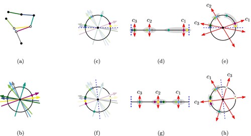We have to account for this cyclic nature. To do so, we can make use of the fact that (a) if we cut the cyclic data and flatten it into a list (as shown in Figure 2) exactly at the boundary between two clusters of an optimal cyclical clustering, then the 1-dimensional clustering results in the same set of clusters and (b) clusters of slopes will never overlap and therefore there are exactly n such candidate gaps (see Figure 2(c,f)) at which we can cut the data and flatten it. This of course creates n calls to the dynamic program, resulting in a total runtime of $\mathcal{O}\left(n^{3}k\right)$. There exist bespoke algorithms for optimal circular clustering like the FOCC algorithm (Debnath and Song, 2021), which achieves an optimal clustering in significantly faster $\mathcal{O}(\mathrm{kn}{\log }^{2}n)$ time. However, we decided to use the dynamic program of Nielsen and Nock since it is (a) easy to implement and (b) not the bottleneck of our approach since any clustering is followed by the construction and subsequent solving of a mixed integer program.

Figure 2. Illustration of how the slopes of the edges of a network (a) are interpreted as a set of circular data (b). Two distinct cases of clustering are shown in (c)–(e) and (f)–(h). We can cut the data (c) & (f) to obtain a 1-dimensional list of data points (d) & (g). After using a k-median clustering algorithm, we obtain an orientation system (e) & (h) from the median of every cluster. It is clear to see that the quality of the clustering is dependent on the choice of cut, e.g. $0^{\circ }$ in (c) or ${94}^{\circ }$ in (f). Note that our data range is only $0^{\circ }$ to ${180}^{\circ }$ and three points have been mirrored in (f) and (h) for illustrative purposes. (a) Example network. (b) Edge slopes. (c) Cut at $0^{\circ }$. (d) 1-dimensional data. (e) Resulting clustering. (f) Cut at ${94}^{\circ }$. (g) 1-dimensional data and (h) Resulting clustering.

During the experiments, however, the above approach turned out to lead to a number of instances, for which, with the orientations resulting from a ${\mathrm{dist}}_G$-optimal clustering, the mixed integer program admitted no solution. Possible reasons for this are discussed at the end of Section ‘Discussion’. Note that since Nielsen and Nock's dynamic programming approach (Nielsen and Nock, 2014) computes an optimal clustering, this is not an issue related to this particular algorithm, but instead an issue of the k-medians clustering itself and it would persist, even if we would use the FOCC algorithm. In contrast, simply sorting all edges by slope and cutting the cyclical order at $0^{\circ }$, lead to orientation systems, for which a solution existed in all cases. All further tables, results and figures, which refer to irregular clustering were computed using the cut at $0^{\circ }$ unless explicitly stated otherwise.

MIP Model

Next, we sketch how the constraints of the MIP model (Nöllenburg and Wolff, 2011) must be modified in order to compute more general $\mathcal{C}$-oriented metro maps for a given arbitrary set $\mathcal{C}$ of k orientations. In our description, we focus on the differences to the octolinear MIP model.

Hard Constraints

The hard constraints comprise four aspects: $\mathcal{C}$-oriented coordinate system, assignment of edge directions, combinatorial embedding, and planarity.

Coordinate System

Every vertex u of G has two Cartesian coordinates in the plane $\mathbb{R}$², specified as $x\left(u\right)$ and $y\left(u\right)$. In order to address vertex coordinates for a flexible number k of orientations, we define a redundant system of k coordinates $z_0,\dots ,z_{k-1}$ which are all real-valued variables in the MIP model and can all be obtained by rotating the x-axis counterclockwise by one of the angles in the orientation system $\mathcal{C}=\{{\theta }_0,\dots ,{\theta }_{k-1}\}\subset [0,\pi )$. We define the coordinate $z_i\left(u\right)$ using $x\left(u\right)$ and $y\left(u\right)$ as $z_i\left(u\right)=\cos \left({\theta }_i\right)\cdot x\left(u\right)+\sin \left({\theta }_i\right)\cdot y\left(u\right)$.

In order to be able to express later that two vertices u, v are collinear on a line with slope in $\mathcal{C}$, we need the orthogonal orientation $z_i^o$ for each coordinate $z_i$. Note that while $z_i^o$ can coincide with other coordinates, this is guaranteed only in a regular orientation system with an even number of orientations. In general, this is not the case and we need to define a second set of redundant coordinates, see Figure 1(a,b,d). Using a rotation by $\pi /2$ we obtain $z_i^o\left(u\right)=-\sin \left({\theta }_i\right)\cdot x\left(u\right)+\cos \left({\theta }_i\right)\cdot y\left(u\right)$.

Edge Directions and Minimum Length

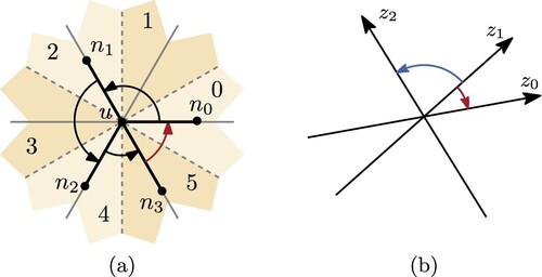
Every edge $(u,v)\in E$ has an original direction in the input layout of G, defined as the direction from u to v. Our $\mathcal{C}$-oriented coordinate system splits the plane into exactly $2k$ sectors numbered from 0 to 2k−1 for each vertex $u\in V$, see Figure 3(a). We store the sector in which an edge $(u,v)$ lies in the input drawing as a constant ${\sec }_u\left(v\right)$ that we call the original sector of $(u,v)$.

Figure 3. (a) For edges $(u,n_3),(u,n_0)$ the direction value decreases from 5 to 0. (b) The difference in angle between the orientations $z_0$ and $z_1$ (red arrow) is significantly smaller than between $z_1$ and $z_2$ (blue arrow). (a) Sector labeling and (b) k = 3, irregular.

Next, we define an integer variable $\mathrm{dir}(u,v)$ to encode the selected direction of the edge $(u,v)$ in a $\mathcal{C}$-oriented solution. The range for $\mathrm{dir}(u,v)$ includes the original sector ${\sec }_u\left(v\right)$ and $s\ge 1$ admissible neighbouring sectors in both directions. The original MIP model (Nöllenburg and Wolff, 2011) uses s = 1, which results in a range of three admissible edge directions for each edge. For each edge $(u,v)$, we define the set $\mathcal{S}(u,v)$ of admissible directions (all index calculations are modulo 2k) as $\mathcal{S}(u,v)=\{i\mid {\sec }_u(v)-s\le i\le {\sec }_u(v)+s\}$.

For each $i\in \mathcal{S}(u,v)$ we define its corresponding direction number as ${\sec }_u^i\left(v\right)$ and define a binary variable ${\alpha }_i(u,v)$ of which only one can be true at any given time (1(1) $\sum _{i\in \mathcal{S}(u,v)}{\alpha }_i(u,v)=1$(1) ). These are then used to assign the correct value of $\mathrm{dir}(u,v)$ (2(2) $\mathrm{dir}(u,v)=\sum _{i\in \mathcal{S}(u,v)}{\sec }_u^i\left(v\right)\cdot {\alpha }_i(u,v)$(2) ). (1) $\sum _{i\in \mathcal{S}(u,v)}{\alpha }_i(u,v)=1$(1) (2) $\mathrm{dir}(u,v)=\sum _{i\in \mathcal{S}(u,v)}{\sec }_u^i\left(v\right)\cdot {\alpha }_i(u,v)$(2) We further define $\mathrm{dir}(v,u)=\mathrm{dir}(u,v)+k$ for the opposite edge $(v,u)$.

To guarantee that the output layout draws the edge $(u,v)$ in the selected direction $\mathrm{dir}(u,v)$ we need to ensure that the variables of u and v for the orthogonal coordinate axis $z_i^o$ are equal, i.e. $z_{\mathrm{dir}(u,v)}^o\left(u\right)=z_{\mathrm{dir}(u,v)}^o\left(v\right)$ (3a(3a) $z_{i^{\prime }}^o\left(u\right)-z_{i^{\prime }}^o\left(v\right)\le M(1-{\alpha }_i(u,v\left)\right)$(3a) ) and that the coordinates $z_{\mathrm{dir}(u,v)}\left(u\right)$ and $z_{\mathrm{dir}(u,v)}\left(v\right)$ differ by at least the minimum edge length $L_{\min }$, i.e. $z_{\mathrm{dir}(u,v)}\left(v\right)-z_{\mathrm{dir}(u,v)}\left(u\right)\ge L_{\min }$ (3b(3b) $z_{i^{\prime }}\left(v\right)-z_{i^{\prime }}\left(u\right)\ge -M(1-{\alpha }_i(u,v\left)\right)+L_{min}\mathrm{if}i<k$(3b) ). (3a) $z_{i^{\prime }}^o\left(u\right)-z_{i^{\prime }}^o\left(v\right)\le M(1-{\alpha }_i(u,v\left)\right)$(3a)   $-z_{i^{\prime }}^o\left(u\right)+z_{i^{\prime }}^o\left(v\right)\le M(1-{\alpha }_i(u,v\left)\right)$  (3b) $z_{i^{\prime }}\left(v\right)-z_{i^{\prime }}\left(u\right)\ge -M(1-{\alpha }_i(u,v\left)\right)+L_{min}\mathrm{if}i<k$(3b)   $z_{i^{\prime }}\left(u\right)-z_{i^{\prime }}\left(v\right)\ge -M(1-{\alpha }_i(u,v\left)\right)+L_{min}\mathrm{if}i\ge k$  Note four things. Firstly, the constraints are created for every $i\in \mathcal{S}(u,v)$. Secondly, we use $i^{\prime }=imodk$, since we only have k coordinates, but $2k$ possible directions. Third, we need to distinguish whether the direction i is smaller than the number k of orientations, in which case u must have a smaller value than v in coordinate $z_i$, or otherwise if $i\ge k$ then v must have the smaller coordinate and we need to invert the difference in (3b(3b) $z_{i^{\prime }}\left(v\right)-z_{i^{\prime }}\left(u\right)\ge -M(1-{\alpha }_i(u,v\left)\right)+L_{min}\mathrm{if}i<k$(3b) ). And fourth, every triple of constraints for which ${\alpha }_i(u,v)=0$ is trivially satisfied by using a sufficiently big constant M in the constraints. Due to (1(1) $\sum _{i\in \mathcal{S}(u,v)}{\alpha }_i(u,v)=1$(1) ), ${\alpha }_i(u,v)=1$ for exactly one index i and only for that index i the constraints have the desired effect on the coordinates.

Combinatorial Embedding

We want to keep the combinatorial embedding, i.e. the topology of the input layout, which translates into preserving the cyclic order of the neighbors of each vertex. This can be expressed by requiring that the edge direction values strictly increase when visiting the incident edges in counterclockwise input order.

There is exactly one exception, namely when going from the last used sector to the first one.

Figure 3(a) illustrates this situation, where the crossover point lies between the neighbors $n_3$ and $n_0$, marked in red. Here we can add an offset of $2k$ instead to make the condition hold. Since this must happen exactly once, we can use binary variables ${\text{β}}_1\left(v\right),{\text{β}}_2\left(v\right),\dots ,{\text{β}}_{\mathrm{deg}\left(v\right)}\left(v\right)$ to select the respective edge pair in Equations (4(4) $\sum _{i=1}^{\mathrm{deg}\left(v\right)}{\text{β}}_i\left(v\right)=1$(4) ) and (5(5) $\mathrm{dir}(v,u_2)+1\le \mathrm{dir}(v,u_3)+2k\cdot {\text{β}}_2\left(v\right)$(5) ). (4) $\sum _{i=1}^{\mathrm{deg}\left(v\right)}{\text{β}}_i\left(v\right)=1$(4)   $\mathrm{dir}(v,u_1)+1\le \mathrm{dir}(v,u_2)+2k\cdot {\text{β}}_1\left(v\right)$  (5) $\mathrm{dir}(v,u_2)+1\le \mathrm{dir}(v,u_3)+2k\cdot {\text{β}}_2\left(v\right)$(5)   $\mathrm{dir}(v,u_{\mathrm{deg}\left(v\right)})+1\le \mathrm{dir}(v,u_1)+2k\cdot {\text{β}}_{\mathrm{deg}\left(v\right)}\left(v\right)$ 

Planarity

For every pair of non-adjacent edges $e=(u,v)$ and $e^{\prime }=(u^{\prime },v^{\prime })$ we need to find (at least) one separation line between e and $e^{\prime }$ in a direction of $\mathcal{K}$ to guarantee that $e,e^{\prime }$ do not intersect. We define a set of $2k$ binary variables ${\gamma }_i(e,e^{\prime })$ for which we require that at least one of them is set to true. (6) $\sum _{i=0}^{2k-1}{\gamma }_i(e,e^{\prime })\ge 1$(6) Now we ensure that every pair of edges $e,e^{\prime }$ has a minimum distance $d_{min}$ in the selected directions, i.e. both endpoints of e have a distance of at least $d_{min}$ to both endpoints of $e^{\prime }$. (7) $\begin{array}{rl}{z}_{i^{\prime }}\left(u^{\prime }\right)-z_{i^{\prime }}\left(u\right)& \ge -M(1-{\gamma }_i(e,e^{\prime }\left)\right)+d_{min}\\ z_{i^{\prime }}\left(u^{\prime }\right)-z_{i^{\prime }}\left(v\right)& \ge -M(1-{\gamma }_i(e,e^{\prime }\left)\right)+d_{min}\\ z_{i^{\prime }}\left(v^{\prime }\right)-z_{i^{\prime }}\left(u\right)& \ge -M(1-{\gamma }_i(e,e^{\prime }\left)\right)+d_{min}\\ z_{i^{\prime }}\left(v^{\prime }\right)-z_{i^{\prime }}\left(v\right)& \ge -M(1-{\gamma }_i(e,e^{\prime }\left)\right)+d_{min}\end{array}$(7) Note that the constraints are created for every $0\le i<2k$, that we use $i^{\prime }=\mathrm{imodk}$ and that the first k sets of these equations look like (10(7) $\begin{array}{rl}{z}_{i^{\prime }}\left(u^{\prime }\right)-z_{i^{\prime }}\left(u\right)& \ge -M(1-{\gamma }_i(e,e^{\prime }\left)\right)+d_{min}\\ z_{i^{\prime }}\left(u^{\prime }\right)-z_{i^{\prime }}\left(v\right)& \ge -M(1-{\gamma }_i(e,e^{\prime }\left)\right)+d_{min}\\ z_{i^{\prime }}\left(v^{\prime }\right)-z_{i^{\prime }}\left(u\right)& \ge -M(1-{\gamma }_i(e,e^{\prime }\left)\right)+d_{min}\\ z_{i^{\prime }}\left(v^{\prime }\right)-z_{i^{\prime }}\left(v\right)& \ge -M(1-{\gamma }_i(e,e^{\prime }\left)\right)+d_{min}\end{array}$(7) ), while the rest needs to invert the differences, e.g. $-z_{i^{\prime }}\left(u^{\prime }\right)+z_{i^{\prime }}\left(u\right)$, since they change sides with respect to direction $z_{i^{\prime }}$.

Soft Constraints

Soft constraints model the aesthetic quality criteria to be optimized in the layout. We adapt the three criteria of the octolinear MIP (Nöllenburg and Wolff, 2011) to arbitrary orientation systems: line straightness, topographicity, and compactness. Each requires a set of linear constraints and a corresponding linear term in the objective function.

Line Straightness

We optimize for line straightness by minimizing the number and angles of bends along the metro lines in $\mathcal{L}$. Firstly, we create a variable $\theta (u_1,u_2,u_3)$ for all pairs of consecutive edges $e_1=(u_1,u_2),e_2=(u_2,u_3)$ along some path $L\in \mathcal{L}$ that represents the cost of a potential bend between $e_1$ and $e_2$ on the metro line L. To assign $\theta (u_1,u_2,u_3)$ we subtract the direction of $e_2$ from the direction of $e_1$. If the edges do not have the same direction, the difference $\mathrm{dir}(u_1,u_2)-\mathrm{dir}(u_2,u_3)$ which we will call $\mathrm{\Delta }{\mathrm{dir}}_{u_1,u_2,u_3}$ will either be positive or negative and $\mathrm{\Delta }{\mathrm{dir}}_{u_1,u_2,u_3}\in [-2k+1,2k-1]$. From the original paper (Nöllenburg and Wolff 2011) we know that $\theta (u_1,u_2,u_3)=min\left\{\right|\mathrm{\Delta }{\mathrm{dir}}_{u_1,u_2,u_3}|,2k-|\mathrm{\Delta }{\mathrm{dir}}_{u_1,u_2,u_3}\left|\right\}$, i.e. $\theta \in [-k+1,k-1]$. Using two binary correction variables ${\delta }_1$ and ${\delta }_2$ we can ensure that θ takes the desired minimal value (8(8) $-\theta (u_1,u_2,u_3)\le \mathrm{\Delta }{\mathrm{dir}}_{u_1,u_2,u_3}-2k\cdot {\delta }_1+2k\cdot {\delta }_2$(8) ), which then lets us define the bend cost function (9(9) ${\mathrm{cost}}_{\mathrm{bends}}=\sum _{L\in \mathcal{L}}\sum _{(u_1,u_2),(u_2,u_3)\in L}\theta (u_1,u_2,u_3)$(9) ). (8) $-\theta (u_1,u_2,u_3)\le \mathrm{\Delta }{\mathrm{dir}}_{u_1,u_2,u_3}-2k\cdot {\delta }_1+2k\cdot {\delta }_2$(8)   $\theta (u_1,u_2,u_3)\ge \mathrm{\Delta }{\mathrm{dir}}_{u_1,u_2,u_3}-2k\cdot {\delta }_1+2k\cdot {\delta }_2$  (9) ${\mathrm{cost}}_{\mathrm{bends}}=\sum _{L\in \mathcal{L}}\sum _{(u_1,u_2),(u_2,u_3)\in L}\theta (u_1,u_2,u_3)$(9)

Topographicity

In order to support the mental map (Misue et al., 1995) of the user, we want the shape of the output drawing to resemble the input drawing as closely as possible. For this we try to preserve the input directions of the edges. Formally, we want to minimize the difference between the input direction and the output direction. However we have to consider the type of orientation system that is in use. Specifically, for aligned and regular orientation systems, we simply minimize $\sum _{(u,v)\in E}\left|\mathrm{dir}\right(u,v)-{\sec }_u(v\left)\right|$. In order to minimize the sum of absolute values we define new variables $\xi (u,v)=\left|\mathrm{dir}\right(u,v)-{\sec }_u(v\left)\right|$ by imposing (10(10) $\mathrm{dir}(u,v)-{\sec }_u\left(v\right)\le \xi (u,v)$(10) ). The topographicity cost function that is minimized is simply the sum over all ξ-variables (11(11) ${\mathrm{cost}}_{\mathrm{topo}}=\sum _{(u,v)\in E}\xi (u,v)$(11) ). (10) $\mathrm{dir}(u,v)-{\sec }_u\left(v\right)\le \xi (u,v)$(10)   $-\mathrm{dir}(u,v)+{\sec }_u\left(v\right)\le \xi (u,v)$  (11) ${\mathrm{cost}}_{\mathrm{topo}}=\sum _{(u,v)\in E}\xi (u,v)$(11) Here every edge $(u,v)$, which is drawn in a sector that deviates from its input sector ${\sec }_u\left(v\right)$ incurs a penalty of exactly the number of deviated sectors (which in our experiments has been capped to at most one and therefore every edge either produces a penalty of 1 or no penalty).

It turns out that this lines up for aligned and regular orientation systems since they use equiangular orientations. In an irregular system on the other hand, a deviation of one sector to the left could be a very small actual angle difference in the produced drawing, while a similar deviation of one sector to the right could, at the same time, mean a large angle difference (see Figure 3(b)). To account for this, we can define an individual sector deviation penalty for every edge and every possible deviation of that edge. Let $e=(u,v)$ be an edge with an input sector ${\sec }_u\left(v\right)$. Then we adapt the constraints (10  $-\mathrm{dir}(u,v)+{\sec }_u\left(v\right)\le \xi (u,v)$  ) as follows. (12) $\begin{array}{rl}\mathrm{dir}(u,v)-{\sec }_u\left(v\right)& \le {\xi }_1(u,v)\\ -\mathrm{dir}(u,v)+{\sec }_u\left(v\right)& \le {\xi }_2(u,v)\end{array}$(12) Now ${\xi }_1>0$ corresponds to a counterclockwise deviation of an edge, while ${\xi }_2>0$ corresponds to a clockwise deviation. We multiply each variable with an individual constant weight to account for the actual angle difference of the corresponding deviation in an irregular orientation system. (13) ${\mathrm{cost}}_{\mathrm{topo}}=\sum _{(u,v)\in E}(w_1^e\cdot {\xi }_1(u,v\left)\right)+\sum _{(u,v)\in E}(w_2^e\cdot {\xi }_2(u,v\left)\right)$(13)

While the penalty weights $w_1^e$ and $w_2^e$ can be chosen freely, we aim to replicate the scale of the aligned and regular systems, where a deviation of $\alpha =2\pi /2k$, i.e. the only available deviation by exactly one sector, equals a penalty of 1. Let β be the angle between two orientations of an irregular orientation system. Then we choose the penalty for an edge, which deviates from one orientation to the other as $w=\text{β}/\alpha =k\text{β}/\pi$.

Compactness

To ensure a compact layout we minimize the total edge length of the output drawing. Here we use that the Euclidean length of an edge $e=(u,v)$ in a $\mathcal{C}$-oriented layout is defined by the maximum absolute value $\left|z_i\right(u)-z_i(v\left)\right|$ in all k coordinates (the projections in all other directions are shorter) which we model by a variable $\lambda (u,v)$. The compactness cost function is the sum of all edge lengths. (14) $z_i\left(u\right)-z_i\left(v\right)\le \lambda (u,v)$(14)   $-z_i\left(u\right)+z_i\left(v\right)\le \lambda (u,v)$  (15) ${\mathrm{cost}}_{\mathrm{length}}=\sum _{(u,v)\in E}\lambda (u,v)$(15)

Objective Function

The objective function to be minimized is composed of the three different terms ${\mathrm{cost}}_{\mathrm{bends}},{\mathrm{cost}}_{\mathrm{topo}}$ and ${\mathrm{cost}}_{\mathrm{length}}$ defined above. Each term can be weighted with factors $f_1,f_2,f_3$ depending on their relative importance. (16) $\mathrm{minimize}{f}_1\cdot {\mathrm{cost}}_{\mathrm{bends}}+f_2\cdot {\mathrm{cost}}_{\mathrm{topo}}+f_3\cdot {\mathrm{cost}}_{\mathrm{length}}$(16)

Improvements

There are several practical improvements to accelerate this MIP (Nöllenburg and Wolff, 2011).

Planarity on demand. The number of planarity constraints (Section ‘Planarity’) grows quadratically with the number of edges, but most of them are never critical as any reasonable layout satisfies them trivially. So they suggested ways of reducing the number of necessary constraints and to add them only on demand, which immediately carries over to our generalized implementation. In practice, whenever we find a new best solution during the iterative solving process of the MIP, we check if any edges cross. If this is not the case, we have found a valid intermediate solution, otherwise, we add planarity constraints forcing each of the two edges to be non-overlapping with all other edges and continue the search.

Contraction of low degree vertices. Another speed-up method is to make use of the assumption that sequences of vertices with degree 2 (chains of edges between interchange or terminal stations) are usually drawn in the same direction. We can therefore remove these edges and replace them with a dummy edge, whose minimal length is set to a large enough value, s.t., all stations can be re-inserted on this edge in a final solution even at its minimal length. To allow further flexibility, we in fact replace each chain of such edges not by one, but by a chain of three edges, s.t., there is enough space for the reinsertion of the stations. Finally, after re-inserting the station on this edge we distribute the stations equally along the chain of three edges to achieve a more well-distributed look in the final map. While the application of this edge contraction is a commonly used method, it stands somewhat in contrast to the goal of accurately representing the original edge direction of each individual edge. It should therefore not be seen as a strict improvement, but rather as a speed-up tool with a trade-off.

Experiments

We performed experiments on real-world metro networks to compare the computational performance and visual quality of the computed metro maps with different linearity systems.

Setup

We generated schematic layouts of the metro networks of Montreal (n = 65, m = 66), Vienna (n = 90, m = 96), Washington DC (n = 97, m = 101), Sydney (n = 173, m = 181), Berlin (n = 242, m = 293) and London (n = 267, m = 320) using aligned, regular and irregular orientation systems with $k\in \{3,4,5\}$ orientations (Berlin and London were restricted to $k\in \{4,5\}$ due to the existence of vertices with degree 7 or 8). All layouts were created with two different weight vectors for the objective function, a more balanced setting $(f_1,f_2,f_3)=(3,2,1)$ and one emphasizing bend minimization $(f_1,f_2,f_3)=(10,5,1)$, resulting in 96 instances in total. For all layouts we added planarity constraints on demand and used s = 1 admissible neighbouring sectors for each original edge direction (recall Section ‘Edge Directions and Minimum Length’). Finally, we contracted chains of degree two vertices as described in Section ‘Improvements’. The experiments were run on a computing cluster with 3 nodes, each with 1024 GB RAM and two 24-core AMD EPYC 7402, 2.80 GHz. All experiments were restricted to a single thread within IBM ILOG CPLEX. The operating system runs a Linux kernel version 4.15.0-208. Our implementation uses IBM ILOG CPLEX 12.8 to solve the integer linear programs as single threads. Each experiment had an allocated available memory space of 32 GB for Vienna, Montreal, Sydney, and Washington and 60 GB for London and Berlin. To reflect a realistic application scenario and to showcase the ability of the MIP approach to compute reasonable results before reaching optimality, we set a time limit of 1 h for every instance. The time limit was chosen as a compromise between an attempt of finding as many optimal solutions to the instances as possible and modeling a reasonable use case which would not require the user to let the solver run over night. To judge the quality and performance of a layout, we use several measurements. Line straightness was measured by the bend cost in the MIP (see Section ‘Soft Constraints’). The sector deviation is a coarse measure of topographicity, counting how many edges are not drawn in their preferred direction (see Section ‘Topographicity’). Sector deviation is measured in total and on average per edge. Another measure of topographicity is the angular distortion, i.e. the actual angular difference between input edges and schematized output edges which is measured on average per edge. Finally, we measure the runtime in seconds and the optimality gap of the best-found solution after the time limit as given by the solver in per cent.

Results

Here we show a representative set of nine layouts of the Sydney metro network in Figure 4 and the performance and quality measurements in Table 1. Additionally a comparison between the three methods of determining the set $\mathcal{C}$ of drawing directions is depicted in Figure 5 for the weight vector $(f_1,f_2,f_3)=(3,2,1)$. The full set of plots and tables for all networks and the alternative weight vector $(f_1,f_2,f_3)=(10,5,1)$ can be found in the supplementary material. The 1-hour time limit for CPLEX was reached by all Sydney instances. Note, however, that during the process of solving the MIP, we have access to intermediate, but possibly suboptimal solutions. Even in instances which run out of time (like Sydney) we tend to find intermediate solutions which are visually already quite close to the final solutions (at the 1 h time limit) after only a few minutes of computation. Since solving these instances as close to optimality as possible increases comparability between instances via the taken measurements, we set a rather long time limit.

Figure 4. Examples of Sydney generated with objective function weights $(f_1,f_2,f_3)=(3,2,1)$ for different $k\in \{3,4,5\}$ and aligned (k-A), regular (k-R) and irregular (k-I) orientation systems. All shown instances reached the time-out limit of 1 h.

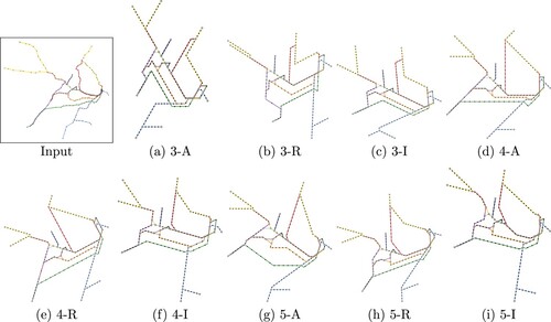
Figure 5. Plots of the results of the experiments for the objective function weights $(f_1,f_2,f_3)=(3,2,1)$. Every metric is shown as a coloured line, the columns are the three orientation systems.

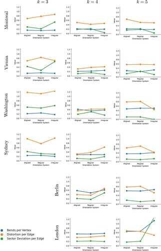
Table 1. Metric results for the Sydney network displaying the results for the different parameters, i.e. the number of available directions (k) and the orientation system (Aligned, Regular, Irregular).

	instance	Sydney
	linearity	k = 3			k = 4			k = 5
weights	orientation system	A	R	I	A	R	I	A	R	I
	bends	42.0	43.0	35.0	49.0	49.0	49.0	63.0	64.0	72.0
	sector deviation	41.0	32.0	29.0	11.0	8.0	18.0	12.0	10.0	14.0
	per edge	0.42	0.33	0.3	0.11	0.08	0.19	0.12	0.1	0.14
	distortion per edge	1.0	0.78	1.03	0.31	0.38	0.62	0.63	0.71	0.43
	time in seconds
$(3,2,1)$	optimality gap	0.2	0.2	0.16	0.13	0.12	0.1	0.11	0.08	0.07
	bends	31.0	32.0	35.0	48.0	47.0	47.0	59.0	59.0	59.0
	sector deviation	36.0	32.0	24.0	8.0	10.0	17.0	12.0	12.0	18.0
	per edge	0.37	0.33	0.25	0.08	0.1	0.18	0.12	0.12	0.19
	distortion per edge	0.88	0.84	1.02	0.29	0.33	0.59	0.65	0.68	0.49
	time in seconds									2216.0
$(10,5,1)$	optimality gap	0.09	0.07	0.05	0.01	0.02	0.01	0.01	0.01	0.0

Note: Metrics are the number of bends, sector deviation (total and per edge), distortion per edge (measured using ${\mathrm{dist}}_{\mathrm{\Delta }}\left(\mathcal{C}\right)$), the runtime in seconds (instances which reached the computation time limit of 1 h are marked with a clock symbol ) and the optimality gap in percent (listed as number between 0 and 1). For one set of objective function weights and linearity k combination the best value across all orientation systems of every metric is bold.

Specific instances in this section will be referred to by name followed by their number of orientations k and the weights $f_1,f_2,f_3$ in parentheses. Our first observation from generalizing the existing model (Nöllenburg and Wolff 2011) is that the MIP model size, i.e. the numbers of constraints and variables scale linearly with the number k of orientations. So as long as k is a (small) constant the asymptotics with respect to the graph size parameters n and m remain the same. Yet, in practice, doubling the size of the model may yield a significant slow-down in the runtime.

Initially comparing the metrics for the two different weight vectors $(3,2,1)$ and $(10,5,1)$ shows that, while the specific values are different, overall trends are very similar, as expected.

Comparing the number of bends, we can see in Table 1 that increasing k leads to a greater number of bends. This can be explained in part by an increase in forced bends, where the probability that consecutive edges in a metro line cannot possibly be drawn in the same direction increases with k. This could be counteracted by increasing the parameter s, i.e. allowing more than two admissible neighbouring sectors for each edge (an action which in turn will have an effect on the time needed to solve the MIP). The difference in bends between the aligned, the regular and the irregular orientation systems is small and when emphasizing the bend cost more (by increasing $f_1$ from 3 to 10), we obtain almost identical values across the board with the exception of the two larger instances Berlin and London, where the irregular system leads to a larger number of bends with an increase of around 11% We observe here already that the irregular system for k = 5 for London obtains very poor metrics overall, indicating that the heuristic determination of suitable directions for the map was not successful for this instance. Unsurprisingly we have almost always fewer bends, when emphasizing the objective function that minimizes bends with the sole exception of the regular Vienna-5 instance, where a reduction in sector deviation offsets the larger amount of bends.

Overall sector deviation decreases or remains stagnant with increasing k with a more pronounced drop from k = 3 to k = 4 than from k = 4 to k = 5. In contrast, the actual distortion per edge of the computed map is smallest for k = 4. This is surprising, since with a higher k and the same allowed discrepancy of one sector to the left or right, one would expect that edges are forced to be closer to their original edge direction. A possible explanation would be that the available directions for a single edge are too restrictive leading to a large number of conflicts and in particular a larger number of edges which have to ‘escape’ to one of the neighbouring sectors. This seems unlikely since as explained above the actual sector deviation per edge is mostly smaller for k = 5 than for k = 4. This leads us to conjecture that for our chosen test instances, the selected angles for the k = 5 orientation systems happened to be less suited for the instances when compared to the angles of the k = 4 orientation systems.

Comparing the aligned and regular orientation system, we can see that, while they are often comparable, in some instances like Montreal-3-(10, 5, 1) there is a significant difference in sector deviation of up to 0.17 per edge. In turn, Washington-4-(3, 2, 1) shows a 0.11 increase in sector deviation per edge for regular systems, indicating that here the heuristically chosen directions are in fact less suitable for a schematic map than the fixed aligned directions.

The comparison with the irregular system looks very similar, although slightly more promising. For some instances (e.g. Montreal, Vienna, and Washington for k = 4, 5), the irregular orientation system is significantly better than the other two. Overall the deviation is comparable and for Berlin-4 it (somewhat surprisingly) tends to be worse than in the aligned setting, with differences of up to 0.3 (average sector deviation per edge).

The general picture of the actual angle distortion is again comparable for most instances between the regular and the aligned setting, with no clear trend visible. The irregular setting is also often close to the other two for this metric, with some notable exceptions. For Sydney-4 and Berlin-4, it is significantly worse, while for Washington-5, Sydney-5, and Berlin-5 the opposite is true. It might be the case that with increasing k, the irregular system is increasing its ability to approximate the slopes in the input in a more fine-grained way. Again, rather unsurprisingly, we increase the angle distortion, when we emphasize line straightness with weights (10, 5, 1). A surprising observation is that angle distortion is generally smaller for k = 4 than for k = 5.

Due to the time limit, runtime results are only comparable between the three smallest instances Montreal, Vienna and Washington. Here too, there is no clear trend. Montreal is solved quickest for k = 3, for Vienna, we see that k = 4 has the lowest runtime, while Washington acutally peforms best for k = 5.

Discussion

Our approach of increasing the topographicity in metro maps through data-driven computation of orientation systems seems to be working for a reasonable number of example instances. Choosing an irregular orientation system is a valid option to increase topographicity, even if the irregular set of slopes is unfamiliar in the context of metro maps. Moreover, we can see that in isolated instances distortion can be lower when restricted to a smaller set of directions, which might be an indication that some input maps lend themselves more naturally to a specific k which is not always the octolinear k = 4 or the highest possible number.

Looking at the actual metro maps produced by our system, we can see one major caveat of our approach to minimize distortion by deciding the directions based on the input. While for most edges we have a very close representative direction in the orientation system, the constraints of the MIP might still force an edge to be drawn in a different sector. In Figure 4(e) the top left branches of the yellow line are drawn in two different directions, despite there being a direction available for the lower branch which is closer to its general direction in the input. However due to the upper yellow branch occupying this direction already the lower branch is drawn in a direction with more topographic distortion, witnessing once more that for an actual layout Δ we have ${\mathrm{dist}}_{\mathrm{\Delta }}\left(\mathcal{C}\right)\ge {\mathrm{dist}}_G\left(\mathcal{C}\right)$.

On a positive note we see that irregular orientation systems can create metro maps resembling the input more closely than typical aligned systems (compare Figure 4(a,c)).

We can also see that most of the layouts which are not using an aligned orientation system do not include the horizontal direction. This might be helpful in labeling these metro maps, since it is difficult to place the visually preferred horizontal labels along a horizontal line with a clear association with a station.

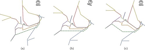
In contrast, if we would want to include one specific prominent direction, such as the horizontal one, we can rotate the map in a post-processing step, such that the orientation closest to horizontal becomes horizontally aligned. It should be noted that such a map is now drawn with orientations that are different to the computed orientation system and therefore has technically a different distortion if the user interprets the map as still being oriented with North upwards. This can then be offset by explicitly adding a compass rose (see Figure 6).

Figure 6. The transit network of Sydney using a 5-linear orientation system. (a) The computed angles of the regular orientation system (5-R) do not include a horizontal angle. (b) This map can be rotated until one direction coincides with the horizontal direction. The original north is indicated with a compass rose. (c) Note that, while the available directions are now the same as in the aligned map (5-A), they are oriented differently during the optimization and therefore the output maps are different. (a) Computed regular map (5-R). (b) Rotated regular map (5-R) and (c) Computed aligned map (5-A).

Lastly we want to discuss the effects of the clustering method for irregular orientation systems. A stated in Section ‘Irregular Orientation Systems’, we aimed to find a suitable irregular orientation system based on the slopes of edges present in the input map. To this end, we employed a 1-dimensional k-medians clustering algorithm, partitioning these slopes into appropriate clusters, which are in turn represented by their median direction. We had to adjust for the circular nature of a set of slopes. We find an optimal k-median clustering by running a 1-dimensional clustering algorithm a linear number of times in order to guarantee a globally optimal solution (see Section ‘Irregular Orientation Systems’).

However, this resulted in some instances in our experiments, whose corresponding MIP models did not admit any feasible solution. One reason for this could be that the resulting irregular orientation systems – unlike regular orientation systems – can contain an orientation c with a large angular distance to its two neighbouring orientations. As a result, the interval of slopes whose closest orientation is c becomes comparatively large. If four or more edges with a shared endpoint all consider c to be their representative orientation, any MIP which allows for a sector deviation of at most 1 (see Section ‘Topographicity’) is necessarily infeasible. We would therefore advise to exercise caution in the use of irregular orientation systems, in particular when the distances between one orientation and its neighbors become large.

In contrast, choosing the (arbitrary) cutting point at $0^{\circ }$ for the input edge slopes resulted in feasible instances for all tested cases. This underlines that the optimality of the clustering of slopes in the input does not necessarily correlate with the actual optimality of an irregular orientation system, but is instead just a coarse proxy. Section ‘Conclusions’ also points out how further research might aim to improve this.

Conclusions

We presented and implemented an adaptation of an existing MIP model for octolinear metro maps (Nöllenburg and Wolff, 2011) that can draw metro maps schematized to any set $\mathcal{C}$ of arbitrary orientations. This is supplemented by a data-driven approach to optimize the set $\mathcal{C}$ based on k-medians clustering of the input edge orientations or by finding the best rotation of a regular orientation system. Finally, we performed, presented, and discussed experiments of our system and its results for different real-world metro maps.

An approach to choose a suitable k for a given input might be to use the smallest k which generates visually appealing layouts in order to find a middle ground between the schematic appearance of the metro map and geographic accuracy. This leads to the general idea, that it is still important for a metro map designer to consider a number of possible layouts in different linearities for a given input network in order to find the most suitable metro map style. Hence our system should not be understood as a stand-alone method to metro map generation, but rather as an automated tool to help pre-select possible candidates for layouts and increase the number of layout settings a designer can explore at low time cost. This pre-selection might be refined in the future if a more global metric to judge the quality of a metro maps is devised.

In future work, we want to include station labeling (Niedermann and Haunert, 2018) for k-linear metro maps. Similarly, there is additional functionality which can be encoded in the MIP, e.g. preventing bends in stations. One motivation for k-linearity is based on the hypothesis that certain linearities are more suited to a particular metro network than others. It would be interesting to test this hypothesis and compare user performance between maps of different linearities with a user study. Further, there is a clear path for additional investigations, when it comes to deriving the drawing directions based on the input. Currently, the clustering is executed after contracting degree-two stations. However, since the goal is to represent all edges as closely as possible, there is a possibility to base the directions on the complete input map instead of the contracted one.

As previously mentioned, the connection between the optimality of the clustering of the edge slopes in the input and the suitability of the corresponding irregular orientation system for a schematic map is unclear. A possibility to improve on this would be to consider a constrained clustering variant, which aims to capture the goal more directly. Since we suspect that the occasional infeasibility of the MIP models stems from neighbouring edges all being clustered in the same cluster and therefore all attempting to be drawn in the same direction, a clustering which constrains neighbouring edges to be grouped into different clusters might yield an improvement.

Another interesting point is to make the derivation of suitable schematization properties even more granular and investigate how locally different linearities and orientation systems could be integrated in the same map. And finally, more design decisions could be based on the input data, e.g. the decision how exactly we should contract the chains of degree two edges. In particular in large transit maps, there are sometimes such chains which form quite generous loops around other edges or geographic obstacles in their input geography, a feature which we might want to preserve to further increase topographicity, but also to avoid representing such a chain with a direct connection between its start and end point which might pose a significant obstacle.

Acknowledgments

The authors thank Maxwell J. Roberts for discussions about non-standard linearity models. The authors acknowledge TU Wien Bibliothek for financial support through its Open Access Funding Programme.

Disclosure statement

No potential conflict of interest was reported by the author(s).

Additional information

Funding

This research has been funded by the Vienna Science and Technology Fund (WWTF) [10.47379/ICT19035]. The first author has also received funding from the European Union's Horizon 2020 research and innovation programme under the HORIZON EUROPE Marie Skłodowska-Curie Actions grant agreement no 101034253.

Notes on contributors

Martin Nöllenburg

Martin Nöllenburg is a Professor in the Algorithms and Complexity Group of TU Wien, Vienna, Austria. He received his PhD and habilitation degrees from Karlsruhe Institute of Technology (KIT), Germany, in 2009 and 2015. His research interests include graph drawing algorithms, computational geometry, information visualization, and computational cartography.

Soeren Terziadis

Soeren Terziadis received his PhD from TU Wien in 2024 and is now a post-doctoral researcher at TU Eindhoven. His research interests include map schematization, computational cartography and complexity of and algorithms for geometric problems.

References

- Barth, L., Niedermann, B., Rutter, I. and Wolf, M. (2021) “A topology-shape-metrics framework for ortho-radial graph drawing” CoRR. abs/2106.05734.
- Bast, H., Brosi, P. and Storandt, S. (2020) “Metro Maps on Octilinear Grid Graphs” Computer Graphics Forum 39 (3) pp.357–367.
- Bast, H., Brosi, P. and Storandt, S. (2021) “Metro Maps on Flexible Base Grids” In Hoel, E., Oliver, D., Wong, R. C. and Eldawy, A. (Eds) Proceedings of the 17th International Symposium on Spatial and Temporal Databases, SSTD 2021 Virtual Event, USA: 23rd–25th August 2021: ACM, pp.12–22.
- Buchin, K., Meulemans, W., van Renssen, A. and Speckmann, B. (2016) “Area-preserving Simplification and Schematization of Polygonal Subdivisions” ACM Transactions on Spatial Algorithms and Systems 2 (1) pp.1–36. Article No. 2.
- Debnath, T. and Song, M. (2021) “Fast Optimal Circular Clustering and Applications on Round Genomes” IEEE/ACM Transactions on Computational Biology and Bioinformatics 18 (6) pp.2061–2071.
- Delling, D., Gemsa, A., Nöllenburg, M., Pajor, T. and Rutter, I. (2014) “On D-regular Schematization of Embedded Paths” Computational Geometry: Theory and Applications 47 (3A) pp.381–406.
- Duncan, C.A. and Goodrich, M.T. (2013) “Planar Orthogonal and Polyline Drawing Algorithms” In Tamassia, R. (Ed.) Handbook of Graph Drawing and Visualization New York: CRC Press, Chapter 7, pp.223–246. https://www.taylorfrancis.com/books/mono/10 .1201/b15385/handbook-graph-drawing-visualization-roberto-tamassia
- Garland, K. (1994) Mr Beck's Underground Map Crowthorne: Capital Transport Publishing.
- KVB (2022) Liniennetzpläne (Accessed: 16th April 2023).
- Merrick, D. and Gudmundsson, J. (2007) “Path Simplification for Metro Map Layout” In Kaufmann, M. and Wagner, D. (Eds) Graph Drawing (GD'06) Vol. 4372: LNCS Berlin: Springer, pp.258–269.
- Misue, K., Eades, P., Lai, W. and Sugiyama, K. (1995) “Layout Adjustment and the Mental Map” Journal of Visual Languages and Computing 6 (2) pp.183–210.
- Neyer, G. (1999) “Line Simplification with Restricted Orientations” In Dehne, F.K., Gupta, A., Sack, J.-R. and Tamassia, R. (Eds) Algorithms and Data Structures (WADS'99) Vol. 1663: LNCS Berlin: Springer, pp.13–24.
- Niedermann, B. and Haunert, J.-H. (2018) “An Algorithmic Framework for Labeling Network Maps” Algorithmica 80 (5) pp.1493–1533.
- Niedermann, B. and Rutter, I. (2020) “An Integer-Linear Program for Bend-Minimization in Ortho-Radial Drawings” In Auber, D. and Valtr, P. (Eds) Graph Drawing and Network Visualization – 28th International Symposium, GD 2020 Vol. 12590: Lecture Notes in Computer Science Vancouver, Canada: 16th–18th September Revised Selected Papers: Springer, pp.235–249.
- Niedermann, B., Rutter, I. and Wolf, M. (2019) “Efficient Algorithms for Ortho-Radial Graph Drawing” In Barequet, G. and Wang, Y. (Eds) 35th International Symposium on Computational Geometry, SoCG 2019 Vol. 129: LIPIcs Portland, Oregon, USA: 18th–21st June 2019: Schloss Dagstuhl – Leibniz-Zentrum für Informatik, pp.53:1–53:14.
- Nielsen, F. and Nock, R. (2014) “Optimal Interval Clustering: Application to Bregman Clustering and Statistical Mixture Learning” IEEE Signal Processing Letters 21 (10) pp.1289–1292.
- Nöllenburg, M. (2014) “A Survey on Automated Metro Map Layout Methods” In Schematic Mapping Workshop Essex, UK.
- Nöllenburg, M. and Wolff, A. (2011) “Drawing and Labeling High-quality Metro Maps by Mixed-integer Programming” IEEE Transactions on Visualization and Computer Graphics 17 (5) pp.626–641.
- Roberts, M.J. (2014) “What's Your Theory of Effective Schematic Map Design?” In Schematic Mapping Workshop Essex, UK.
- Roberts, M.J., Gray, H. and Lesnik, J. (2017) “Preference Versus Performance: Investigating the Dissociation Between Objective Measures and Subjective Ratings of Usability for Schematic Metro Maps and Intuitive Theories of Design” International Journal of Human-Computer Studies 98 pp.109–128. https://www.sciencedirect.com/science/article/pii/S1071581916300751?casa_token=dwLOcQylLoQAAAAA:CiybIvxmu-IvvY52K3yZJ5it173JuzArKuDdy2ElZO4medB2eoRlRf_1hQ4NHYg6ax6CwAncWQ
- Roberts, M.J., Newton, E.J., Lagattolla, F.D., Hughes, S. and Hasler, M.C. (2013) “Objective Versus Subjective Measures of Paris Metro Map Usability: Investigating Traditional Octolinear Versus All-curves Schematics” International Journal of Human-Computer Studies 71 (3) pp.363–386.
- Wolff, A. (2007) “Drawing Subway Maps: A Survey” Informatik – Forschung Und Entwicklung 22 (1) pp.23–44.
- Wu, H.-Y., Niedermann, B., Takahashi, S. and Nöllenburg, M. (2019) “A Survey on Computing Schematic Network Maps: The Challenge to Interactivity” 2nd Schematic Mapping Workshop Vienna, Austria.
- Wu, H.-Y., Niedermann, B., Takahashi, S., Roberts, M.J. and Nöllenburg, M. (2020) “A Survey on Transit Map Layout – From Design, Machine, and Human Perspectives” Computer Graphics Forum 39 (3) pp.619–646.