Large-Scale Generation of Transit Maps from OpenStreetMap Data

ABSTRACT

We investigate the automatic generation of transit map overlays (either geographically correct or schematic) for the entire planet from OpenStreetMap (OSM) data. To achieve this, we first extract relevant transit line geometries (together with their line name, and, if present, colour) from OSM using SPARQL queries against an RDF version of the OSM data. The queries are run against our SPARQL engine QLever. In the second step, we build a global line network graph where every edge is labelled with the lines travelling through it. The components of this network graph are then rendered as a transit map using tools and methods developed in previous work. Final maps are delivered as vector tiles to an interactive web map, from which individual network graphs (in a GeoJSON format proposed in this work) can be downloaded for research purposes. The vector tiles are also freely available. We briefly describe the methods used in each pipeline step, evaluate the speed and quality of our approach and discuss possible shortcomings.

KEYWORDS:

• Metro map drawing
• transit maps
• automated map generation
• OpenStreetMap data
• tiled maps
• map design

Introduction

Since the days of Harry Beck, transit maps have mostly been created manually by professional map designers (Garland 1994; Wu et al. 2020). The primary focus was on static maps, either distributed in print or electronically. These maps are typically schematic, and the classic octilinear design (network segment orientations are multiples of ${45}^{\circ }$) is still prevalent. In the late 1990s, the graph drawing community started to investigate the problem of drawing such maps automatically. The following questions were investigated: (1) How can graphs be drawn in an octilinear fashion? (2) Which hard criteria should a transit map fulfil? (3) Which soft criteria should be optimized? Several methods have since been proposed (see below). A set of soft and hard criteria, first described by Nöllenburg (2005), has since been generally accepted. The important sub-problem of finding an optimal line ordering of lines travelling through network segments has also been identified very early by Benkert et al. (2006).

The methods presented in the literature so far typically assume a network graph $G=(V,E)$, embedded in ${\mathbb{R}}^2$, as input. V is a set of stations, E is a set of network segments, and each $e\in E$ is labelled with a set of lines $L(e)$ travelling through it. Evaluation is done on a hand-picked set of networks, although a set of standard networks has emerged over the years. Neither the input nor the output format are well-defined, and only a single static network map is rendered. Several open practical problems remain:

(1)	Obtaining network data It remains unclear how a clean input graph G can be generated from noisy, real-world input data.
(2)	Comparability Because no standard input and output formats exist, it is still hard to consistently compare different approaches.
(3)	Usability Static rendered images are hard to explore, especially for large maps.
(4)	Scalability It is unclear whether existing approaches scale to larger networks.

In this work, we aim to tackle these problems. We describe a pipeline to render (schematic) transit maps for the entire world. Using tools developed in previous work, we describe how network data can be obtained from OpenStreetMap (OSM) and demonstrate the scalability of our existing transit map rendering suite LOOM¹. We extend LOOM to be able to render vector tiles and offer a web map² of our results. Our web application can also be used to download network graphs for individual components. As a data serialization format for network graphs, we propose GeoJSON (Butler et al. 2016) (see below).

Our primary goal was not to produce perfect maps, but to demonstrate that a fully automated generation of transit maps on a global scale is possible with the techniques described in this work, and to establish a pipeline and an interchange format that might allow researchers to replace individual components with novel approaches. With this in mind, we consider the following our main contributions:

• We describe a pipeline to render global transit maps from OSM data. Previous work only considered individual steps of this process on manually selected networks which were curated by hand or generated from schedule data. The method for finding optimal line orderings has been previously published (Bast et al. 2018, 2019), but also with a focus on manually selected networks. The method for map schematization has also been previously published (Bast et al. 2020, 2021).

• We present a web application offering transit maps for the entire planet.

• The vector tiles produced in this web application are freely available³.

• We propose a GeoJSON-based format for exchanging public transit line graphs. All line graphs extracted from OSM can be downloaded from our web app.

• We evaluate the performance and scalability of our approach and discuss quality shortcomings using selected examples from our map.

• All of our tools are available as open source software⁴.

Throughout this work, we call a map of a public transit network a transit map. A transit map may either be schematic or geographically correct. The input network graph $G=(V,E)$ is called the line graph. Each edge $e\in E$ is labelled with the set $L(e)$ of lines using the edge, as well as a polyline $P(e)$ describing the geographic course of the edge. For greater flexibility, we allow non-station nodes and maintain a set $S\subseteq V$ of station nodes. A label function $s(v)$ labels a station node with its name.

Our full pipeline consists of the following steps: (1) We first obtain a line graph G from OSM data using a SPARQL query on an RDF database. (2) We then extract a so-called free linegraph, without overlapping segments. A free line graph is a line graph in which each intersection or stop of the transit network is (within a threshold) merged into a single node, and in which each segment has enough space around it to later render all lines passing through it without overlap. (3) For better readability, we find optimal permutations of the lines on each segment, minimizing the weighted number of line crossings and line separations. (4) Optionally, the line graphs are then schematized, using an octilinear, geo-octilinear (approximated geographical courses), or orthoradial layout. (5) We render the maps as vector tiles, which can be easily included in web maps. Network segments are rendered by first freeing the area around nodes, and then rendering each line on each segment offset to the segment's centre line. The freed node areas are then reconstructed with Bézier curves (we call these line connections). Then the station markers are rendered.

Related Work

Map Construction

Our line graph construction method described below is strongly related to existing work on map construction. In the latter case, the goal is to construct a road network (where are the intersections, where are the roads) from a collection of strongly overlapping vehicle GPS traces. In our case, we have a collection of overlapping geographical transit vehicle paths from which we want to construct the underlying topological transit network (where are the intersections, where do lines branch, where are the stations, where are network segments and which lines travel on them). Existing map construction methods may be classified into point clustering, intersection linking, and incremental construction methods (Ahmed et al. 2015). Point clustering methods operate directly on the GPS sample points. These are first clustered (using e.g. k-means clustering based on the geographic distance) (Biagioni and Eriksson 2012). The clusters are then connected based on the original GPS input traces. Such methods have previously been investigated by Edelkamp and Schrödl (2003), Schrödl et al. (2004), Davies et al. (2006), and Biagioni and Eriksson (2012). Instead of clustering all input points, intersection linking first reconstructs the network intersections and then connects these intersections, again based on the original GPS traces. Such methods have been investigated by Karagiorgou and Pfoser (2012), and Xie et al. (2017). Incremental techniques start with an empty map and insert GPS traces iteratively. The basic idea is to merge neighbouring sample points under a threshold distance during this process. A method based on dense input trace sampling was first described by Rogers et al. (1999). A similar and refined method was later described by Cao and Krumm (2009). Instead of simply merging nearby sample points, the currently inserted trace may also first be (partially) map-matched to the existing map (Ahmed and Wenk 2012). The method used to construct a free line graph, first described by Brosi (2022), can be considered an incremental construction technique. It does not use the map-matching described by Ahmed and Wenk (2012) but uses the greedy approach of selecting the nearest sample point as a merge candidate.

Automated Metro Map Drawing

Our work is also strongly related to previous work on automated metro map drawing, in particular to the sub-problems of finding optimal orderings of the lines traversing through network segments, and the drawing of schematic maps. For a comprehensive recent survey on automated metro map drawing, we refer to Wu et al. (2020).

Our method for the line-ordering optimization problem is based on previous work on the MLCM (metro line crossing minimization) problem, first introduced by Benkert et al. (2006). In this original formulation, line crossings were only allowed along network segments (see below for details). Bekos et al. (2007) described a polynomial algorithm for a special case and proved the NP-hardness of another variant of MLCM. Other special-case algorithms for MLCM and variants were later described by Asquith et al. (2008), Nöllenburg (2009), and Argyriou et al. (2010). In 2013, the NP-hardness of the raw MLCM problem was proven (Fink and Pupyrev 2013). The proof can be modified to also work for MLNCM (Brosi 2022).

In contrast to previous work, our method only allows line crossings at nodes. In this form, it was first described by Bast et al. (2018) and later refined (Bast et al., 2019). The problem was called the metro line node crossing minimization problem (MLNCM), and a weighted variant (MLNCM-W) was also introduced. In MLNCM-W, they may only cross at nodes, but there may be non-station nodes. Bast et al. (2018) also described a problem variant which additionally punishes line separations (MLNCM-WS). Algorithms using a similar idea as our greedy search with lookahead were described by Groeneveld (1989) and by Pupyrev et al. (2016).

Regarding the automated generation of schematic maps, early methods have been described for the road-network case by Elroi (1988a), Elroi (1988b), Avelar and Müller (2000), Ware et al. (2006), Anand et al., (2007), and Li and Dong (2010) or for single polylines by Neyer (1999). Schematic transit maps were first studied by Hong et al. (2004), Stott and Rodgers (2004), and Hong et al. (2006). In this configuration, the problem is usually called metro map drawing. An approach based on finding octilinear embeddings using an ILP was described in (Nöllenburg 2005). There, the set of soft and hard constraints typically used in metro map drawing methods was introduced. Several follow-up works built on this method (Nöllenburg and Wolff 2011; Milea et al. 2011; Wu et al., 2012). Our own method was first described in Bast et al. (2020), and later refined in Bast et al. (2021). It also builds on the soft and hard constraints described by Nöllenburg (2005) and is based on finding an optimal image of an input graph in a grid graph. Batik et al. (2022) extended this method to work with arbitrary template graphs. Orthoradial layouts have also been investigated by Barth et al. (2017), Niedermann and Rutter (2020), and Bast et al. (2021).

Existing Transit Map Projects

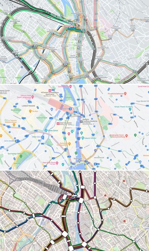
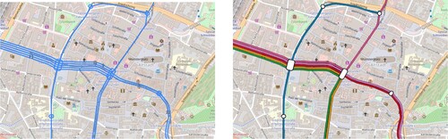
We are not aware of any previous research work on providing transit maps covering the entire world. There are, however, existing global transit layers. Both HERE Maps and Google Maps offer such layers as map overlays, although with an often disappointing quality (see Figure 1). These layers also do not offer schematic transit maps, but can only show geographically correct line courses. Existing global public transportation map tiles for OpenStreetMap (e.g. OpenRailwayMap⁵ or TransportLayer⁶) focus on the physical track layout and do not offer a view in the style of a classic transit map.

Figure 1. The tram network of Zurich on the transit overlay of HERE Maps (top), on Google Maps (middle), and on our geographically correct map rendered from raw OpenStreetMap data (bottom).

Some projects exist that aim to provide metro maps under open licenses or provide software to achieve this. For example, Open Metro Maps⁷ offers a map editor and import scripts for OpenStreetMap data and GTFS. It also strives to develop an interchange format for rendered metro maps⁸. However, the maps still have to be edited mostly manually. The project also appears to be no longer under active development. Another project, metrolinemap.com⁹ offers a world-wide collection of manually selected metro-maps. The maps are manually created coloured overlays of the geographical line courses. No automatic bundling of overlapping lines, optimization of line orderings, or schematization is done.

OpenStreetMap RDF Data

We extract the line graphs from OpenStreetMap data cast to the Resource Description Framework (RDF). The RDF models data as subject-predicate-object triples, or, equivalently, as a directed labelled multigraph (often called a knowledge graph), where each node models an entity (either a subject or an object), and each directed edge models a predicate relationship between two entities. The edge labels are also often called relations. For more details on how to cast OSM data to RDF, and how RDF data can be queried, see below. The RDF dumps used in this work were generated by osm2rdf ¹⁰, a tool developed by us in previous work (Bast et al. 2021). An alternative tool for generating RDF data from OSM is Sophox¹¹. Stadler et al. (2012) also describe a tool to generate RDF data from OSM. The general problem of building RDF triples from any spatial data source has been investigated by Kyzirakos et al. (2018) and Patroumpas et al. (2019). To query the OSM RDF data, we use the QLever¹² SPARQL engine (Bast and Buchhold 2017). QLever provides efficient query processing also on large knowledge graphs, efficient context-sensitive autocompletion (Bast et al. 2022), and a GUI to display results on a map. The latter also includes a GeoJSON download functionality. We use these GeoJSON exports as input for our rendering pipeline.

Obtaining Network Data

Our pipeline requires the physical transportation network as GeoJSON data. After a quick introduction on how public transit networks are modelled in OSM, this section describes how such a GeoJSON file can be obtained with a single SPARQL query.

Public Transit Networks in OpenStreetMap

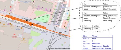
OSM data consists of nodes (point-like objects), ways (sorted lists of nodes modeling polylines and polygons), and relations (groups of other objects). Each type of object can have arbitrary key-value pairs. To maintain consistency, these key-value pairs are described in a comprehensive Wiki¹³. Public transit networks are modelled in OSM as route=* relations, which group all ways and nodes associated with a single transit line. Possible values for the route attribute are for example bus, tram, subway, or light_rail. These relations are usually outfitted with a ref=* value holding the line's short name and a colour=* value giving the line's colour. The route=* relations may also contain the stop nodes served by the respective line, or even the stop platforms, although we ignore the latter. Figure 2 gives an example.

Figure 2. A route=tram relation in OSM (blue) for tram line 3 (direction ‘Munzinger Straße’) in Freiburg, Germany, with its tags (simple key/value pairs). Relations in OSM group multiple spatial objects, in this case, the tracks the line travels on, the stop points, and a platform, which can again all be tagged. We only show the tags relevant for this work. The relation itself is for example tagged with the line label (ref=) and its colour (colour=). The stop position is tagged with the station name (name=). We ignore platform objects in this work.

Querying OpenStreetMap

We require only a small subset of the OSM data which describes public transit. There are three established ways to filter OSM data (Bast et al. 2021): (1) Using custom code to parse and filter raw OSM dump files. (2) Using tools to filter raw OSM dump files (e.g. osmfilter or osmconvert). (3) Loading the data into a database management system (DBMS) to query it (e.g. a generic DBMS like PostgreSQL or OSM-specific systems like OverpassAPI).

As described above, our pipeline uses SPARQL queries on an RDF dump of the entire OSM data, generated by our tool osm2rdf .

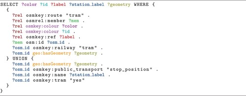
The standard query language for RDF data is SPARQL. In its basic form, a SPARQL query specifies a graph pattern, which can be seen as a small knowledge graph template, where some of the nodes and edges are replaced by variables. The goal of a SPARQL engine is then to find all subgraphs matching that template, and for each match return the values matching the variables. Figure 3 shows a SPARQL query to retrieve the OSM ways of all tram networks, together with all station/stop nodes marked as serving trams. A full list of queries used in this work can be found online in our evaluation setup¹⁴. This query is then run against the SPARQL engine QLever, loaded with the complete OSM RDF data¹⁵. Using the QLever map UI, we then download the query result as GeoJSON data.

Figure 3. A SPARQL query to retrieve the tram networks on earth. Answering this query with QLever took under 1 second.

Network Topology Extraction and Interchange Format

The data extracted from OSM describes the physical layout of lines in a transportation network. As seen in Figure 4, such a network is not suited for rendering a transit map. Because each line has its own geometry, and because most lines run in two directions on different tracks or different sides of the road, lines will overlap in the final map. Additionally, stations are usually modelled as many individual stop positions in OSM, which is not how stations are usually presented in a transit map. This section describes how we transform this network data into a clean, overlap-free line graph representing the topological network, called the free line graph. The general process is shown in Figure 5. Each edge should be labelled with the lines travelling through it and should leave enough space on the left and right for rendering these lines. Additionally, similar stations should be aggregated.

Figure 4. Left: The tram lines of Freiburg, Germany, as extracted from OpenStreetMap (OSM), with the city centre enlarged. Top right: A transit map rendered from this raw data is not very informative (overlapping lines are hidden, and stops are rendered multiple times). Bottom right: The transit map produced by our pipeline.

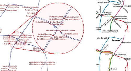
Figure 5. Left: An input line graph with many overlapping edges and station nodes. Middle: Overlap-free line graph. Overlapping segments have been merged into single edges. A node $u^{\prime }$ was added where lines $\{A,B\}$ and $\{C,D\}$ branch. Right: A transit map rendered from this line graph using our pipeline.

Our general approach is as follows: first, we build a support graph in which edges within a distance of $\hat{d}$ are merged. This step uses a tailored map-construction approach and ignores station nodes. Second, we infer line turn restriction. This step is important to correctly render intersection nodes where one or more lines branch into multiple network segments. Last, we cluster station nodes based on their name and distance, and insert a single cluster node at the most fitting position in the support graph.

Support Graph Construction

The steps of our approach are shown in Figure 6. We start with an initially empty support line graph $H_0$ and an input line graph G. The edges of G are sorted incrementally by their length, yielding an edge list $e_1,\dots ,e_n$. The polyline $P(e_i)$ of an $e_i$ is then densely sampled using a sampling length l (we used $l=5m$). This yields a list $p_1\dots p_l$ of coordinates. This list of coordinates is then used to insert $e_i$ into $H_{i-1}$, yielding the intermediate support graph $H_i$. For each sample point $p_k$, the nearest node v in $H_0$ within a distance threshold $\hat{d}$ is retrieved from a geospatial index based on an R-Tree. The position of v is then moved to the average of the previous position and $p_k$. If no node v within $\hat{d}$ is found, a new node $v_k$ at $p_k$ is inserted. Otherwise, we set $v_k=v$. Then, if k > 1, we add an edge $f=\{v_{k-1},v_k\}$ to $H_0$ and set $L(f)=L(e_i)$. If such an edge f was already present, we set $L(f)=L(f)\cup L(e_i)$. To avoid sub-sampling the geometry of an edge by always merging $p_k$ with $v_{k-1}$, we maintain a blocking set B of the last $\hat{d}/l$ inserted nodes for $e_i$. If all n edges have been inserted, we contract degree 2 nodes in $H_n$ (if the adjacent edges have matching lines).

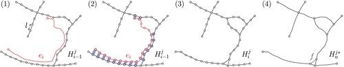
Figure 6. Incremental support graph construction. (1) An edge $e_1$ that is about to be inserted into the support graph $H{}_{i-1}^j$. (2) $e_1$ is densely sampled, and pairs of sample nodes and nearby graph nodes are identified. (3) These pairs are contracted, resulting in a graph $H{}_i^j$. (4) All remaining nodes of degree 2 are contracted as well.

Repeated Construction Until Convergence

Because we insert the edges $e_1,\dots ,e_n$ iteratively, we may miss some merge opportunities. To mitigate this, we apply the described procedure repeatedly in rounds, using the final $H_n$ after each round as the input for the next round. We stop as soon as the edge length gap $|1-L^{\prime }/L|$ is smaller than $0.2\text{\%}$. Here $L=\sum _{e\in E}\mathrm{len}(P(e))$ is the sum of all input edge polyline lengths at the beginning of a round, and $L^{\prime }$ is the value of that sum at the end of the round. The threshold of $0.2\text{\%}$ was empirically determined via experiments on six datasets of bus, tram and light rail networks, which included a manual inspection of the map quality (in particular the number of artefacts remaining). For lower thresholds, we did not observe any noticeable change in the map quality.

Artefacts, Line Creep, and Intersection Smoothing

If an edge $e=\{u,v\}$ in $H_n$ has a length below the sampling rate l, and if it is shorter than any adjacent or surrounding edge, it will be reproduced exactly during any subsequent support graph construction. As e appears in the sorted edge list before any surrounding edge, node u will yield a new node at exactly the same position, and node v will not be merged with u, as u is in the blocking list B of e. To avoid such artefacts, we contract such edges after each iteration.

Another problem is that two input edges e and f that meet at an obtuse angle will be interlaced (see Figure 7 for an example). This may lead to a new edge h between the original e and f with $L(h)=L(e)\cup L(f)$. As the reconstructed edges e and f will again meet h at an obtuse angle, the segment containing the lines of both e and f will grow with each iteration, until the lines on the original edges e and f are completely merged into a single segment. We call this line creep. To avoid it, we extend our blocking set B. Let $p_1$ be the first sampling point of an edge $e_i$ to be inserted into $H_{i-1}$, and $p_l$ be its last sampling point. Given a candidate node v (at position $p_v$) for some sampling coordinate $p_k$ of $e_i$, we add v to B if $\alpha \cdot \mathrm{dist}(p_k,p_1)\le \mathrm{dist}(p_k,p_v)$ or $\alpha \cdot \mathrm{dist}(p_k,p_l)\le \mathrm{dist}(p_k,p_v)$. That is, if $p_k$ is – within a factor of α – nearer to the first or last sampling node of e than to $p_v$, we block v. We choose $\alpha =\sin (\pi /4)$: assuming that $p_1$, $p_k$ and $p_v$ form a right triangle with the hypotenuse $\stackrel{\leftarrow ----\to }{p_1,p_k}$, then $v\in B$ if $\stackrel{\leftarrow ----\to }{p_k,p_1}$ and $\stackrel{\leftarrow ----\to }{p_k,p_v}$ meet at an angle greater than or equal ${45}^{\circ }$.

Figure 7. Line creep during our map construction process. In the example, edge e with $L(e)=\{A\}$ meets a part of $H_i$ that was sampled from an edge f with $L(f)=\{B\}$ at an obtuse angle. The insertion of the (densely sampled) e might merge sample nodes in such a way that a small edge segment is created that shares the original lines of e and f. We mitigate this by preventing a merge with existing nodes if a previously inserted node of e is nearer by a factor of at least α.

Edge geometries at large intersections will also often have visually unpleasing zig-zag patterns (Figure 8). To avoid this, we iterate over each node v in the final support graph and crop the polyline of each adjacent edge at a distance of $\hat{d}$ to v. Node v is then moved to the average position $p_{\mathrm{avg}}$ of all resulting adjacent edge polyline endpoints. The new $p_{\mathrm{avg}}$ is then reconnected to each of the polylines.

Figure 8. Left: The green input graph produced unsteady edges in the constructed free line graph. We crop the adjacent edge polylines at intersection nodes at a distance $\hat{d}$ and then connect them again (right).

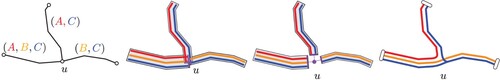
Inferring Line Turn Restrictions

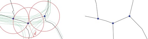
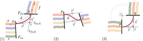
So far, we have assumed that all lines follow simple paths. This is not always the case, and Figure 9 (a transit map of the so-called Chicago loop) gives three examples. In the maps in the middle and on the right, all lines except the green one have a node, where more than two segments of that line are connected and this correctly models the real course of each of these lines (which indeed each goes in a loop). In the map on the left, there are two additional such ‘branching’ nodes for the red line and the pink line, yet these are not correct, but an artefact of our construction of the support graph. In road networks, a connection between networks segments that exists but should not be used in route planning is called a turn restriction, and we will also use that term here.

Figure 9. Left: Chicago loop without line turn restrictions. At large intersections (marked red), matching lines in adjacent segments are connected, although in reality there is no connection. Middle: Same map, with line turn restrictions which prohibit these connections. Right: Same map, but with unordered lines.

Consider two edges e and f connected at a node u in the support graph H constructed thus far. For each line l running over these edges, we want to check whether they are indeed connected at this point in the original input graph G. However, that is not straightforward because the input line graph G contains many edges (all with potentially slightly different courses) that were merged to form e and f in the support graph H. See Figure 10, which shows both the edges of the support graph and of the input line graph. To solve this, we track the merged original edges through the construction process of the support graph. For each edge e in the support graph H, we then have a set $M(e)$ with the original edges in G that were merged into e.

Figure 10. Illustration of the procedure to determine whether a line l that runs over edges e and f should be connected in the final transit map. Both the support graph H (black) and the original input graph G (colored) are shown. The handle nodes in H relevant for the connections between e and f are marked α and β. The corresponding sets of handle nodes in G are marked $\mathcal{A}$ and $\mathcal{B}$. For example, for the red line A, we compare the cost of the shortest path between α and β in H (which is relatively short) with the cost of the shortest path between $\mathcal{A}$ and $\mathcal{B}$ in G using only the red edges (which is relatively long because the two lines are not actually connected around u). For line A, we would therefore infer that there is no connection between e and f for that line (a ‘turn restriction’).

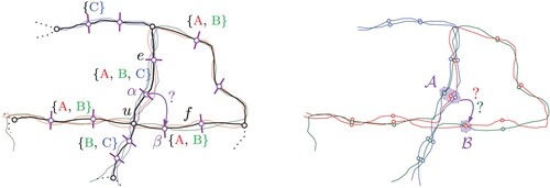
We cut each edge in H into three parts of equal length and add two handle nodes at the cutting points. In Figure 10, the two handle nodes relevant for determining which lines on e and f should be connected or not are marked α and β. We then project the handle node position onto the edges from the original input graph. In Figure 10, for the two handle nodes α and β from the support graph H, this yields sets of handle nodes $\mathcal{A}$ and $\mathcal{B}$ in the original input graph G.

For each line $l\in L(e)\cap L(f)$, we then compute the cost $c(l)$ of the (undirected) shortest path on the input graph G between $\mathcal{A}$ and $\mathcal{B}$, where we only allow edges to be used that belong to line l¹⁶. We compare $c(l)$ to the length c of the shortest path between α and β in the support graph H. We draw a connection for line l between e and f in the final transit map if and only if $|c-c(l)|\le t$, for a threshold parameter t. For all our transit maps, we set $t=500\mathrm{m}$.

Station Insertion

To re-insert stations into our support graph H, we first group the input stops S using a straightforward approach. Two stops $s_1$ and $s_2$ belong to the same cluster if they are part of the same input graph component, and have exactly matching string labels.

After clustering, we retrieve for each cluster A the set $O=\bigcup _{s\in A}\mathrm{adj}(s)$ of all original edges adjacent to any station in a. For each cluster A, we calculate the station centroid c and retrieve each edge and each node from H within a threshold distance to c. The candidate edges and nodes are then ranked based on the number of merged original edges on the edge itself (for edge candidates) or on all adjacent edges (for node candidates) shared with A. We say that a candidate serves these original edges. The stop is then inserted at the candidate of the highest score. In some cases, the candidate position does not serve all original edges in O. We then continue with the next candidate that serves at least one of the remaining edges, and add an additional station there. This process continues until all edges O have been served.

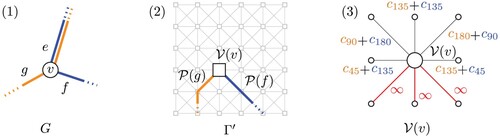
Line Graph GeoJSON Format

To share data between individual steps of or pipeline, and to also enable a consistent evaluation of future research methods in metro map drawing, we propose a simple GeoJSON-based file format for free line graphs. Edges are represented as LineString features, and nodes as Point features. LineStrings and Points form a graph via node ID attributes.

In particular, we propose the Point and LineString attributes described in Table 1. Each point has a node ID and can optionally hold a station_label and a non-unique station_id, used to group multiple station nodes. Each LineString can hold a list of transit lines, described by an ID, as well as an optional color and a label. Lines can be globally defined on the FeatureCollection level, and may be referenced by their ID in a LineString Alternatively, they can be defined directly in the LineString. Color and label of lines with the same ID can then be overwritten per edge. Lines may also hold a node ID which describes the line's direction on this edge, which essentially models a directed multi-graph. If no such direction node ID is given, the line travels in both directions. Points may list lines not extending from adjacent node node_from to adjacent node node_to in the excluded_conn attribute.

Table 1. Attributes of our proposed line graph GeoJSON format.

This format can be readily inspected using standard GIS tools. It can also be easily extended by additional attributes, e.g. by providing more style options to lines using CSS rules. As mentioned above, GeoJSON line graph files for individual networks can be download from our web GUI.

Line-Ordering Optimization

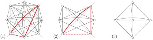
As mentioned above, we produce our final map by rendering all lines on a network that share the same segment of the network next to each other, with a distinct offset for each line. The offsets correspond to an ordering of the lines and which ordering is chosen is crucial for the readability of the final map. Figure 9 gives (on the right) an example of a transit map with a suboptimal line ordering. This problem has been identified early in the context of metro map drawing. In its original formulation, as the Metro Line Crossing Minimization (MLCM) problem, the number of line crossings is minimized, and line crossings are only allowed on edges, not on nodes (Bekos et al. 2007). Figure 11 provides an example for this on the left. The authors' intuition behind this was that crossings should not be hidden behind station nodes. However, with crossings occurring only along edges, it remains unspecified where exactly these crossings should be rendered in the final transit map (note that edge geometries can be long). Additionally, real-world transit maps often hide crossings behind large station markers or place crossings at non-station nodes. For these two reasons, we only allow crossings at nodes. Figure 11 provides an example for this on the right.

Figure 11. A line graph G with line orderings in the MLCM formulation (left) and our MLNCM formulation (right). Under MLCM, crossings are not allowed to occur in nodes and must happen on edge e. Under MLNCM, crossings are only allowed at nodes.

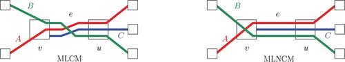
Weighted Minimization of Line Crossings and Separations At Nodes

A variation of MLCM which only allows lines crossings at nodes, then called the Metro Line Node Crossing Minimization (MLNCM) problem, was introduced in Bast et al. (2018). For an example, see Figure 11, right. In a weighted variant (MLNCM-W), crossings can be weighted per node and line pair. As seen in Figure 12, only minimizing the number of crossings is also not enough to achieve visually pleasing maps. Lines that travel next to each other through the network should do this for as long as possible. To achieve this, we introduced the concept of also minimizing weighted line separations (Bast et al. 2018). Let $e=\{u,v\}$ and $f=\{v,w\}$ be two adjacent edges, both containing lines $l_1$ and $l_2$ (that is, $l_1\in L(e)\cap L(f)$ and $l_2\in L(e)\cap L(f)$). A line separation between $l_1$ and $l_2$ occurs at v if $l_1$ and $l_2$ are placed next to each other in e, but not in f, or vice versa. See Figure 12 for examples.

Figure 12. All four line orderings produce four crossings ($\mathrm{C}:4$). The drawing at the bottom right looks best because it also minimizes the number of line separations ($\mathrm{S}:0$).

MLNCM-WS considers the following problem: given a line graph $G=(V,E,L)$, find a set σ containing permutations ${\pi }_e$ for each $L(e)$. These permutations should optimize the sum of all induced crossings and separations, weighted by functions $w_{||}(v,l_1,l_2)$ (separation penalty per node and line pair) and $w_{\times }(v,l_1,l_2)$ (crossing penalty per node and line pair).

Finding Optimal Line Orderings

Finding an optimal line ordering solution in the original MLCM formulation was proven to be NP-hard by Fink and Pupyrev (2013). The problem remains NP-hard in the MLNCM and MLNCM-WS variants (Brosi 2022). In this work, we optimize the line orderings using a combination of previously established reduction rules, a simple greedy optimization algorithm, and a subsequent local search to polish the solution. This heuristic has been experimentally shown to be very close to optimal on real-world instances (Brosi 2022).

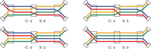
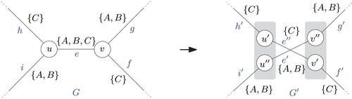
Line Graph Reduction

In previous work, we developed a set of graph transformation rules that reduce an input line graph G to its core problem graph $G^{\ast }$ (Bast et al. 2019). These reduction rules can be applied in polynomial time. Any core problem graph $G^{\ast }$ is still an MLNCM-WS problem instance, and any optimal line ordering solution for $G^{\ast }$ can be transformed in polynomial time into an optimal line ordering solution G. The application of these reduction rules typically results in a core graph $G^{\ast }$ of much lower search space size. Intuitively, the reduction rules implicitly compute optimal partial line orderings on edges. The most basic of these transformation rules is the contraction of degree-2 nodes adjacent to two edges with the same lines travelling through it (if a node with cheaper crossing and separation weights is adjacent). An example of a more sophisticated transformation rule is given in Figure 13. For details on these transformation rules, we refer to Bast et al. (2019) and Brosi (2022).

Figure 13. Left: Excerpt of a line graph G, where an unavoidable intersection of two line bundles $\{A,B\}$ and $\{C\}$ occurs over 2 nodes u and v. For simplicity, we assume uniform crossing and separation weights. Right: G is transformed into a graph $G^{\prime }$ in which nodes u and v have been split. It is easy to see that any optimal line ordering solution for $G^{\prime }$ can be transformed into an optimal line ordering solution for G. In some sense, the intersection between $\{A,B\}$ and $\{C\}$ has been made explicit.

Greedy Search with Lookahead

After we have reduced the line graph to its core, we optimize the individual graph components using an informed greedy search. This greedy search only considers line crossings and is not guaranteed to yield optimal results.

We first define an ordering $e_1,\dots ,e_n$ on the input edges E (we simply used the input ordering), and iterate over the $e_i$ in this order. For such an edge $e_i=\{u,v\}$, we say w.l.o.g. that u is the reference node. We now consider two lines $l_1$ and $l_2$ from $L(e)$ for which no ordering has been established yet and sort them so that their order is locally optimal w.r.t. u. There are four cases we have to consider: (1) $l_1$ and $l_2$ branch at u into two edges f and g. (2) $l_1$ and $l_2$ extend into the same edge $f=\{v,w\}$, and we have settled an ordering for $l_1$ and $l_2$ in $L(f)$. (3) Like (2), but without a settled ordering for $l_1$ and $l_2$ in $L(f)$. (4) None of the above. In the case of (1), the circular ordering of f and g around u implies a crossing-free ordering of $l_1$ and $l_2$. In the case of (2), an ordering of $l_1$ and $l_2$ in $L(e)$ which does not cause a crossing at u is induced by the ordering of $l_1$ and $l_2$ in $L(f)$. In the case of (3), we follow the common path of $l_1$ and $l_2$ through G in the direction of node w until we find a node inducing an ordering. In the case of (4), we say that $l_1$ and $l_2$ are not comparable and check whether they are comparable w.r.t. node v. If they are, we base they ordering on v. If not, we finally conclude that they are incomparable.

These rules describe a strict weak ordering < on the lines of $L(e)$. We sort $L(e_i)$ accordingly and continue to the next edge until we have processed all edges.

In the unweighted MLNCM case, where all lines follow simple paths and end at degree 1 nodes, this algorithm produces an optimal solution (Brosi 2022). For the weighted case, we simply base the ordering of two lines $l_1$ and $l_2$ on an edge $e_1$ on the adjacent node with a lower crossing cost. Although not necessarily optimal, this produced good results in our experiments.

Local Search Using Simulated Annealing

To further refine the solution, we use simulated annealing. For a given line ordering solution σ, let $\theta (\sigma )$ be the target function (the sum of all weighted crossings and separations induced by σ). We additionally define a neighborhood $N(\sigma )$ which consists of all solutions that can be constructed from σ by swapping a single line pair on some edge. A simple local search would always chose the neighbour ${\sigma }^{\prime }$ with lowest $\theta ({\sigma }^{\prime })<\theta (\sigma )$ in each iteration. To leave local optima, we additionally use a temperature T which decreases over time. $T_i$ is the temperature at iteration i. We use $T_0=1,000$. At each iteration i, $T_i$ is set to $T_0/i$, and we randomly choose a ${\sigma }^{\prime }$ from $N(\sigma )$. If $\theta ({\sigma }^{\prime })<\theta (\sigma )$, ${\sigma }^{\prime }$ is chosen. Otherwise, ${\sigma }^{\prime }$ is chosen with probability $P(\sigma ,{\sigma }^{\prime },T_i)=\exp ((-\theta ({\sigma }^{\prime })-\theta (\sigma ))/T_i)$.

Map Schematization

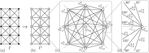
The pipeline described so far will produce maps in which line segments follow their geographical course¹⁷. To also produce schematic maps, we use a technique first described in (Bast et al. 2020). This technique is based on finding optimal metro map images of an input graph G in a template grid graph $\mathrm{\Gamma }=(\mathrm{\Psi },\mathrm{\Omega })$. Γ was originally restricted to regular octilinear grid graphs and was later extended to hexalinear and orthoradial settings (Bast et al. 2021).

Each node v of G is assigned an image node $\mathcal{V}(v)\in \mathrm{\Psi }$, and each edge e of G is assigned an image path $\mathcal{P}(e)=({\psi }_0,\dots ,{\psi }_{n-1})$, ${\psi }_i\in \mathrm{\Psi }$. Together, they form the metro map image of $G$ in $\mathrm{\Gamma }$. To preserve the topology, we require as hard constraints that two image paths are node-disjoint (they are allowed to share first and last nodes) and that the circular edge orderings around nodes in G are preserved in their images. Note that because Γ is based on a grid, we can also ensure a minimum distance between both image nodes and image paths by adjusting the grid size. This ensures that the map density of the final map is not too high.

To further polish the map appearance, the following soft constraints should be optimized: (1) The node displacement in the image should be minimized. (2) The total edge path length in the image should be minimized. (3) The number and acuteness of bends in the image should be minimized. This is sometimes called path monotonicity.

This section describes how optimal schematic metro map images can be computed using iterative shortest-path calculation in an extended version of Γ. We also show how this technique can be used to produce schematic maps which approximate the geographical line courses. As is typical in metro map drawing, we contract all input nodes of degree 2 before schematization and later insert them equidistantly onto the final map.

Finding Optimal Metro Map Images

As shown in Figure 14, we first extend Γ by adding port nodes to each original grid node Ψ. For each direction in which a line might leave Ψ, we add a port. In our example, we use an octilinear grid and thus add eight port nodes. These port nodes are pairwise connected with each other by adding bend edges. Each port node is additionally connected to the original node by a sink edge.

Figure 14. Extended nodes in our template octilinear grid graph. Each node has port nodes for each possible direction, sink edges connecting port nodes and the original grid node, and edges modelling turns when passing through the original grid node.

Modelling Edge Weights

We now focus on finding image nodes $\mathcal{V}(u)$ and $\mathcal{V}(v)$, as well as an image path $\mathcal{P}(e)$, for a single input edge $e=\{u,v\}$ using a single shortest-path computation in the extended grid graph ${\mathrm{\Gamma }}^{\prime }$. To model displacement costs of u and v, we first base the sink edge weights on the distance $d(v,\mathcal{V}(v))$ between v and its image node, again weighted by a parameter $w_m$. To minimize the total edge path length, we set the weight of each horizontal and vertical grid edge to 1. To avoid favouring diagonal edges, and even slightly favour horizontal and vertical lines, we set the cost of diagonal edges to 1.5. To penalize acute bend angles, we give bend edges a weight based on the bend angle they describe.

A single bend edge modeling an acute turn might be replaced by a bend edge path consisting of edges modeling bends of higher angle. This would compromise our penalty system. For example, in Figure 15(1), a ${45}^{\circ }$ degree bend edge is replaced by a ${135}^{\circ }$ bend edge followed by a ${180}^{\circ }$ bend edge. As can be seen in Figure 15(2) and in Figure 15(3), the problem gets less severe for grid graphs with fewer allowed directions and vanishes for grid graphs with only four allowed directions (e.g. orthoradial grids). For graphs with eight allowed directions, let $w_{180}=0\le w_{135}\le w_{90}\le w_{45}$ be the desired penalty weights of bends of the specified angle. Then for $a=w_{45}-w_{135}$ the following bend weights will not allow any shortcut: $w_{180}^{\prime }=w_{180}+a,w_{135}^{\prime }=w_{135}+a,w_{90}^{\prime }=w_{90}+a,w_{45}^{\prime }=w_{45}+a$ (Bast et al. 2020). To avoid distorting the edge length penalty, we subtract a from each grid edge weight.

Figure 15. Extended grid nodes and possible bend edge shortcuts in the octilinear setting (1), a hexalinear setting (2), and the orthoradial setting (3). Figure adapted from Bast et al. (2021).

Optimization Problem

It is easy to see that the shortest path through ${\mathrm{\Gamma }}^{\prime }$ connecting two original grid nodes will optimize the sum of the used grid edges and bend penalties. It will thus produce the path that optimizes the sum of the edge weights and weighted bends. As the sink edge weights are set to the respective displacement costs, we can also include them in the optimization by computing the shortest path between $\mathrm{candidatesets}$ $U\subseteq \mathrm{\Psi }$ and $V\subseteq \mathrm{\Psi }$. It is easy to see that if $U\cap V\ne \mathrm{\varnothing }$ (as is the case for $U=V=\mathrm{\Psi }$), the shortest such path of 0 cost would always be a single node in $U\cap V$. We hence forbid single node paths. However, it is then still unclear how the node displacement costs for nodes in $U\cap V$ should be modelled. An easy solution is to transform ${\mathrm{\Gamma }}^{\prime }$ into a directed graph. This allows modelling the displacement costs for U on the outgoing sink edges, and the displacement costs for V on the incoming sink edges. In this work, however, we use an alternative technique and simply ensure that $U\cap V=\mathrm{\varnothing }$ by constructing them from a Voronoi diagram: grid nodes closer to u are added to U, and grid nodes closer to v are added to V.

To find optimal images of an entire input graph G, one last thing remains: we must also penalize edge bends that do not occur along an image edge path, but between image paths of edges adjacent in G which share a common line. For each pair e, f of adjacent edges at some input node v, let ϕ be the angle at which their image paths through Γ meet. We then add the cost $\sum _{e,f\in \mathrm{adj}(v{)}^2}{w}_{\varphi }|L(e)\cap L(f)|$ for each $v\in V$.

Given then an input graph G and a template grid graph Γ, we want to find the image of G in Γ which optimizes the following target function: (1) $t(\mathcal{V},\mathcal{P})=\sum _{e\in E}c(\mathcal{P}\left(e\right))+\sum _{v\in V}(d(v,\mathcal{V}(v))w_m+\sum _{e,f\in \mathrm{adj}(v{)}^2}{w}_{\varphi }|L(e)\cap L(f)|),$(1) where $c(\mathcal{P})$ is the cost of the image path $\mathcal{P}$. As a template grid graph Γ, we used an octilinear grid graph covering the bounding box of the input graph. The grid cell size was chosen to be the average distance between stations in the input graph. For the orthoradial setting, we used a special orthoradial grid graph (Bast et al. 2021).

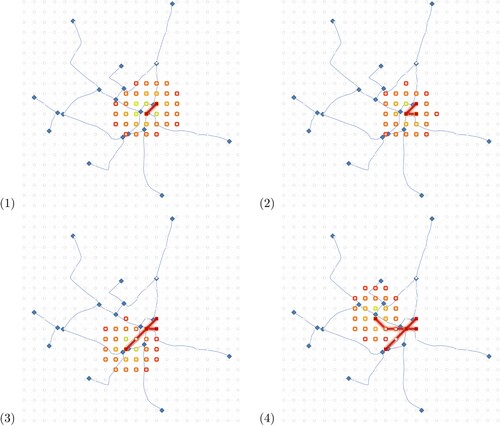
Iterative Shortest Path Calculation

In Bast et al. (2020) and Bast et al. (2021), we describe Integer Linear Programs (ILPs) to produce metro map images which optimize Equation (1(1) $t(\mathcal{V},\mathcal{P})=\sum _{e\in E}c(\mathcal{P}\left(e\right))+\sum _{v\in V}(d(v,\mathcal{V}(v))w_m+\sum _{e,f\in \mathrm{adj}(v{)}^2}{w}_{\varphi }|L(e)\cap L(f)|),$(1) ). As the optimization times tend to be very large (multiple hours even for intermediate networks like the Berlin S-Bahn network), we focus on a heuristic approach to quickly find optimal metro map images in the template graph, as first described by Bast et al. (2020).

We first establish an ordering $e_1,\dots ,e_{|E|}$ on the input edges. We then iteratively search for a shortest path $\mathcal{P}(e)$ through Γ connecting candidate sets U and V for input edge $e_i=\{u,v\}$. As described above, the sink edge costs for nodes in U and V are set to the displacement costs for u and v, respectively. The first node of $\mathcal{P}(e)$ is set as $\mathcal{V}(u)$, the last node as $\mathcal{V}(v)$. If an image node for a node u was already established in a previous iteration, we consider this image node settled and simply set $U=\{\mathcal{V}(u)\}$ (Figure 16). In (Brosi 2022), several possible edge orderings were described and evaluated, with no clear winner. We used all methods described there and chose the metro map image with the best objective function value.

Figure 16. The first four iterations of our approximate metro map image construction. The input line graph is depicted in blue, the metro map image in the template grid graph is depicted in red.

To preserve the input graph topology, we use the following techniques: first, to prevent that image paths cross, we set the cost of a grid edge in Γ to infinity as soon as it is used by an image path. For non-planar template grid graphs (e.g. an octilinear graph), we also set the cost of crossing edges to infinity. Second, we preserve the circular edge ordering around an input node v by setting any sink edge around $\mathcal{V}(v)$ which corresponds to an edge position violating the circular input edge ordering to infinity (Figure 17).

Figure 17. (1) Input line graph node v with adjacent edges e, g, f. (2) Image paths $\mathcal{P}(g)$ and $\mathcal{P}(f)$ have been found. (3) To consider bend penalties between adjacent paths, we offset the sink edge cost with the bend penalty. To maintain the original circular edge ordering around v, we block the sink edges already used, and the sink edge that would place $\mathcal{P}(e)$ between $\mathcal{P}(g)$ and $\mathcal{P}(f)$. Figure adapted from Bast et al. (2020).

To prevent stalling of this greedy construction process, several heuristics are applied (Brosi 2022 provides a detailed list). If no image is found using the approach above, we reduce the grid cell size by $10\text{\%}$, and try again.

Local Search and Constraint Relaxation

To give the metro map images a final polish, we additionally apply a local search. Given an image $(\mathcal{V},\mathcal{P})$, we move each image node to all of its adjacent grid nodes (if free) and re-route all adjacent image paths. Of all such node movements, the one that yields the greatest improvement is taken. If no improvement is possible anymore, the local search stops. Recall that we contracted all degree-2 nodes before starting the construction process. To prevent image paths that are too short to insert all contracted nodes again (which would lead to a high map density an compromise readability), we additionally add spring forces to each image path during the local search phase.

To enable the local search to fix topology violations, we also employ constraint relaxation during the iterative computation of the image paths. Instead of setting blocked edge weights to infinity, we choose a very large fixed value, allowing our incremental approach to produce maps with topology violations.

Approximating Geographical Line Courses

To produce schematic maps which approximate geographical line courses, we simply offset the original grid edge costs by the weighted quadratic distance of the grid edge to the geographical course of the currently routed input edge.

Tiled Map Rendering

As we aim to produce transit maps covering the entire planet, rendering the map to a single raster or vector image would be impractical. We instead opted to deliver tiled maps in this work, which is the standard way to create web maps.

Vector Tiles

A map tile is an image covering $256\times 256$ pixels of a map in a given resolution. The Tile Map Service¹⁸ (TMS) standard defines how these tiles can be accessed via a URL. Tiles are accessed via a URL ending with /<z>/<x>/<y>.<ext>, were <z> is a zoom level (usually 0–22), <x> is the tile's x coordinate, <y> is the tile's y coordinate, and <ext> is the tile image format extension. If the web mercator projection is used, the globe is covered by $2^z\times 2^z$ tiles on zoom level z.

Classic web map tiles are raster images, usually PNG. To allow better map interaction (e.g. hover and click effects) and to also deliver high-quality maps between zoom levels, we extended our render tool transitmap to deliver vector tiles. We chose to use the MapBox vector tiles standard¹⁹, as it is the prevailing standard for vector tiles and is supported by most major web map libraries. Instead of storing raw RGB pixel values, vector tiles describe map objects (points, lines, polygons) via a small set of drawing operations (MoveTo, LineTo, and ClosePath). These drawing operations, together with their target coordinates, are given relative to the upper left corner of the tile and are encoded in 32-bit integers. Each tile can hold several layers of objects, and each object can have arbitrary key-value attributes. The tiles are serialized using Protocol Buffers²⁰ and then served via HTTP.

Map Rendering

Our rendering process, as outlined in Figure 18, consists of 4 steps: (1) For each $e=\{u,v\}\in E$, all lines $L(e)$ are offset around the centre line $P(e)$, based on a predefined line width and line spacing. The resulting line bundles span a polygon. We call the polygon side adjacent to u the node front for u. At each node, all adjacent node fronts are moved along the original centre line of their edge until they to not overlap anymore. (3) Extending lines at each node are connected using cubic Bézier curves. (4) Station markers are rendered over station nodes. After the rendering process is finished, we have a collection of open polygons representing the lines of our final map and closed polygons representing the stations.

Figure 18. Rendering a line graph. First, lines are rendered offset around the edge polyline. Then, node areas are freed by extended adjacent node fronts. Afterwards, line connections in the freed node areas are reconstructed using Bézier curves.

It is not obvious how the control points of the Bézier curves should be placed. Consider a line A that goes from an edge e to an edge f via node u. Let p be the position of A on the node front $F_{\mathrm{eu}}$, and let q be the position of A on the node front $F_{\mathrm{fu}}$. We then determine the overall direction of A at both node fronts by sampling a point 5 m before the node front. At each node front, we then compute line segments of length $|p-q|$ going in this direction (Figure 19).

Figure 19. Reconstruction of line connections in freed nodes using Bézier curves.

If the resulting line segments $t_{\mathrm{fuA}}$ and $t_{\mathrm{euA}}$ intersect at a point i, we average the length of segments pi and qi. Let δ be this average, and let $k=4/3(\sqrt{2}-1)$. We then add two control points $p^{\prime }$ and $q^{\prime }$ at a progression of $k\cdot \delta$ of the extended lines, starting from p and q, respectively, and draw a cubic Bézier curve over $p,p^{\prime },q^{\prime },q$. If the resulting line segments do not intersect, we add $p^{\prime }$ at a progression of $k\cdot t_{\mathrm{euA}}$, and $q^{\prime }$ at a progression of $k\cdot t_{\mathrm{fuA}}$. A nice property of our chosen k is that the cubic Bézier curve approximates a circular arc if i exists and pi and qi have the same length.

To finally produce the vector tiles per zoom level z, we insert all rendered polygons into a spatial grid index. For each populated cell c, we then compute the x, y coordinates of all tiles that intersect that cell on zoom level z. If a polygon intersects the tile at x, y, we crop it to the tile's bounding box and add it to the tile. Note that we do not produce empty tiles.

Vector tiles only deliver raw vector graphics and come without any styling information. Figure 20 shows a map rendered with and without styling. Styling has to be done on the client side (usually a web map). To make it easier to quickly generate maps from the tiles produced by our tool, we output line widths and colours as attributes in our vector tiles.

Figure 20. Left: Unstyled vector tiles layered above OpenStreetMap tiles. Right: Styled vector tiles.

Experimental Evaluation

As mentioned above, we extended existing implementations of the methods described earlier to handle large input graphs. Using the pipeline described in the previous sections, we generated four maps covering the entire world for (1) all tram lines (tram), (2) all subway and light rail lines (subway), (3) all commuter rail lines (commuter) and (4) all long-distance rail lines (long-dist). For each map, we first extracted the relevant OSM data using appropriate SPARQL queries against an RDF dump of the entire OSM data. The raw input dataset sizes are given in Table 2. We then used the LOOM tools topo, loom, octi, and transitmap to generate tiles for a geographically accurate variant (geo), an octilinear variant (octi), an octilinear variant approximating geographical line course (octi-geo), and an orthoradial variant (orthorad). To make the dataset more manageable, we broke the input graph into its distance-based components. Two nodes are in the same such component if they are connected by a path, or if their distance is less then 10 km.

Table 2. Dimension of our input graphs extracted from OSM and of the constructed free line graphs. $|S|$ is the number of stations, $|V|$ the number of nodes, $|E|$ the number of edges. C is the number of distance-based graph components, M the maximum number of lines per edge.

	Input Graph			Free Graph
	$|S|$	$|V|$	$|E|$	$|S|$	$|V|$	$|E|$	C	M
tram	181.3k	457.1k	137.9k	21.9k	23.9k	24.9k	384	18
subway	91.5k	259.7k	84.1k	15.5k	17.7	18.9	319	11
commuter	98.8k	365.3k	133.2k	4.9k	5.5k	5.6k	74	18
long-dist	90.8k	1.5M	690.2k	1.9k	2.8k	3.1k	23	171

Our complete evaluation setup, including all SPARQL queries used to obtain the network data, can be found online²¹. The free line graphs produced by our tool can also be downloaded (per network component) from this web app. The tiles produced in our experiments are available for free²².

In this section, we list the running times of each individual step for each map and discuss the overall map quality as well as shortcomings of our approach.

Performance

The running times of each individual pipeline step for our tram, subway, commuter, and long-dist maps are given in Table 3. We used the same input data, and the same constructed topological graph for all map layouts. Note that we generated tiles for each of the standard zoom levels. For brevity, we only list the running times for zoom level 14 in Table 3. We used the same parameters for the free line graph construction (graph), line ordering optimization (order) and schematization (octi) on each zoom level, so the running times were equivalent. For the rendering part, the running times were comparable across all zoom-levels, although the running times for very high zoom levels ($>18$) tended to be higher because of the large number of tiles that had to be written. Overall, we were able to render global tiles for all test networks, and all layouts, in under 2 hours. This enables us to periodically update our tiles.

Table 3. Performance of each step in our pipeline, for all our test datasets and test layouts.

	query	trans.	free	schem	order	render	total	topo-errs	schem-fail
tram	2.1s	13.4s	10.2m	–	1.5m	31.1s	12.5m	–	–
-octi				38.1s	1.0m	32.0s	12.6m	2	0
-geo-octi				5.9m	1.2m	36.8s	18.2m	4	0
-orthorad				4.3m	1.2m	29.4s	16.5m	277	0
subway	1.9s	8.1s	13.5m	–	8.1s	19.0s	14.1m	–	–
-octi				2.2m	6.1s	16.1s	16.2m	33	0
-geo-octi				5.1m	7.2s	19.1s	19.2m	8	0
-orthorad				9.1m	23.0s	26.1s	23.6m	2.5k	0
commuter	2.3s	9.7s	25.8m	–	13.1s	5.0s	26.3m	–	–
-octi				6.1m	5.1s	3.1s	31.2m	2	0
-geo-octi				4.9m	11.2s	4.1s	31.2m	3	0
-orthorad				6.7m	18.1s	3.0s	33.1m	65	0
long-dist	8.7s	37.1s	1.6h	–	3.3m	20.2s	1.7h	–	–
-octi				1.1m	1.7m	3.1s	1.7h	5	0
-geo-octi				1.7m	1.7m	4.1s	1.7h	0	0
-orthorad				15.3m	1.5m	21.1s	1.9h	256	0

Note: query is the answer time to the SPARQL query, trans. the transfer time of the SPARQL query, free the time to extract the free line graph, schem the schematization time, order the line ordering optimization time, render the time required for rendering, total the sum of these times. Under topo-errs, we give the number of topological constraint violations of the schematic map. Under schem-fail, we give the number of network components for which no schematic drawing was found.

Particularly challenging was the memory consumption of the schematization step. Because we construct a grid graph covering the entire input graph, it was impossible to layout the entire dataset together (because the grid graph would have covered the entire world). Instead, we process each distance-based component separately.

The memory consumption of the free line graph extraction for long-dist was also problematic. Because our method is based on a dense sampling of the input lines every l metres, even a single international rail line may produce hundreds of thousands of sample points, which are all held in memory. We reduced the maximum memory consumption to under 100 GB by setting the sample rate distance from $l=5\mathrm{m}$ to $l=10\mathrm{m}$ for long-dist. Additionally, we created the free line graph separately for each distance-connected component.

Map Quality

The quality of our maps can be inspected online²³. Figures 21, 23, and 24 also give some examples. For an evaluation of the approximation errors introduced by our heuristic method for optimizing the line orderings, we refer to Bast et al. (2019) and Brosi (2022), where we compared the target function values of optimal line ordering solutions obtained via Integer Linear Programming (ILP) to our heuristic methods. For a similar evaluation of the approximation errors introduced by our heuristic method for drawing schematic maps, we refer to Bast et al. (2020) and Bast et al. (2021), where we fully optimized the target function given in Equation (1(1) $t(\mathcal{V},\mathcal{P})=\sum _{e\in E}c(\mathcal{P}\left(e\right))+\sum _{v\in V}(d(v,\mathcal{V}(v))w_m+\sum _{e,f\in \mathrm{adj}(v{)}^2}{w}_{\varphi }|L(e)\cap L(f)|),$(1) ) using ILP and compared both the target function values and the drawing to our heuristic approaches. The respective ILPs are also described in these publications.

Figure 21. Left: Orthoradial map overlay of the Vienna tram network. Right: 171 rail lines tagged in OSM entering Zuoying station in Kaohsiung, Taiwan.

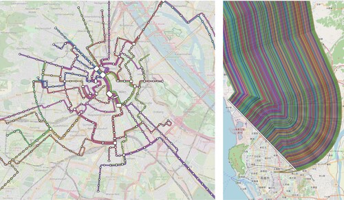
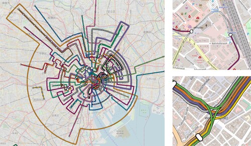
Figure 22. Geographically correct map overlay of the Tokyo subway network.

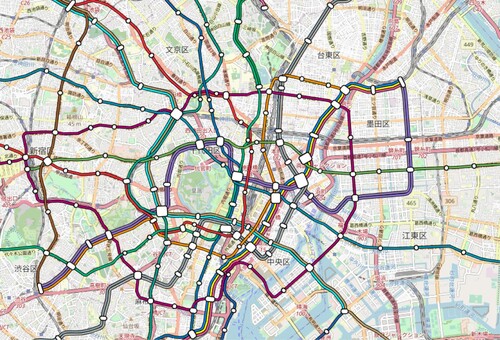
Figure 23. Octilinear map overlay of the long-distance rail network of Europe. Note that it is non-trivial to filter OSM data for long distance rail lines. For this map, we used lines tagged as either service=national, service=long_distance, service=high_speed, or highspeed=yes. In many parts of Europe (e.g. Italy, Spain, or the United Kingdom), tags classifying train routes as long distance are rare.

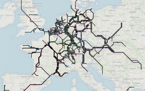
Figure 24. Left: Topology violations and large detours in the orthoradial map of the Toyko subway network. Top right: Inconsistent tagging lead to a missing segment in the Zurich tram network. Bottom right: Incorrectly reconstructed line turn restrictions in the Stuttgart light rail network.

We are aware that a thorough evaluation of the aesthetic quality and usability of our maps is missing from this work. However, this would require a detailed user study, which we consider out of scope for this article, especially given the enormous number of maps that would have to be inspected (for the tram networks alone we created a map covering 375 individual networks). Also note that an automatic evaluation of the map quality, which would be more realistic here, is still an open research problem and listed as one of the challenges in the recent survey by Wu et al. (2020). Nevertheless, we briefly describe several problems with both our approaches in this section.

Problems with the OSM data mainly consisted of missing public transit lines, missing line colours (very often, the network simply does not use colours), and inconsistent tagging. If colours were missing, we assigned random colours (as in the map for Vienna in Figure 21, left). An example for inconsistent tagging can be seen in Figure 24, left. Here, a small part of the Zurich tram network was tagged as a narrow gauge railway (instead of a tram railway), leading to a missing segment in our tram map. Other problems included inconsistent tagging of e.g. network types. For example, the Berlin S-Bahn network is tagged as light_rail, although it arguably is a commuter railway.

Sometimes, the amount of data contained in OSM was excessive. For example, the Taiwan high-speed rail link between Taipei with Kaohsiung has nearly 200 individual line relations. This resulted in the line bundle shown in Figure 21, right.

As seen in Figure 23, some of our maps still show areas of very high density, which makes them very hard to read. Increasing the cell size of the template grid graph would mitigate this issue. However, we noticed in our experiments that our heuristic approach to map schematization produces an increasing amount of topological errors if the template grid size is too large. Using integer linear programming would allow us to also find optimal maps in this case, but with unrealistically high running times (we were not able to produce an optimal solution for the Europe long-distance network in under 12 hours). A alternative approach would be to preprocess the input graph and enlarge areas of very high density, for example by using a simple spring embedding.

Many of the problems we encountered were caused by the construction of the free line graph. In particular, the reconstruction of the line turn restrictions described above did not always work. In Figure 24, middle, for example, the green line does not extend from the south segment to the northeast segment. The main cause was that we so far do not extract the direction of individual lines from OSM. During the routing step of the line turn restriction generation, it is then possible for the shortest path to make a 180${}^{\circ }$ turn, returning a false positive. We tried to mitigate this problem by penalizing full turns, but only with limited success, as this sometimes prevented line turns that occurred in the real world. As we remove lines which end at non-station nodes, this sometimes resulted in lines missing from segments. We plan to fully consider line directions from OSM in future versions of our tiles. As our maps sometimes include historical or special service lines (which run only on special occasions or infrequently) it also seems necessary to filter them out.

Considering the dataset size, the number of topology errors added to our schematic maps was surprisingly low for the octilinear layouts. However, for the orthoradial setting, the number was significantly higher, with over $2,500$ topology errors introduced in the orthoradial subway map. Another problem with the orthoradial maps was that, in order to avoid topology errors, routed image paths sometimes took large circular detours at the outside of the map. This can for example be seen in the orthoradial Tokyo subway map shown in Figure 24, right. Another problem with the schematic maps was that small edge artefacts left from the free line graph construction were enlarged during the schematization. Here, additional cleanup rules seem to be necessary.

For network types where large distances between lines using the same network segments are possible (e.g. long-distance rail lines entering a large station), our merge threshold was sometimes not large enough, resulting in half-merged patterns. Also, the free line graph tends to create unsteady edge geometries at these positions. Additional smoothing would help to produce a cleaner look.

Our maps also lack labels so far. We have implemented a labeller in our tool transitmap in previous work, but so far it only works for the SVG output. We plan to add the labelling to the vector tiles in the near future.

Lastly, we have only rendered maps for individual network types. It would be highly interesting to render maps combining several network types. For geographically correct maps, it may be sufficient to only alter the line width in the rendered map based on the type. For the schematic layout, however, we fear that the combined maps are too complex to be layout together. Here, hierarchical approaches could be promising. The basic idea would be to first layout the network type of highest priority, and later layout sub-networks of lower priority for each graph face in the existing layout.

Conclusion

We described an end-to-end pipeline for rendering tiled transit maps from OpenStreetMap for the entire world. Using previously developed tools and techniques, our pipeline consisted of an extraction of relevant data from OpenStreetMap (OSM) using SPARQL queries on an RDF dump of OSM, a map construction step to extract a free network line graph, a step to find the most readable line ordering on rendered map segments, an optional schematization step which also supported approximating geographical line courses, and a final rendering step which was extended to deliver vector tiles. With this pipeline, we created a global web map for tram, subway, long-distance and commuter rail networks. We gave an evaluation of the running times of our pipeline, using different schematic layouts, and also discussed the quality of the rendered maps. Clearly, our work can only be considered a first step towards a fully automated generation of high-quality global transit maps. Problems remain with the free line graph construction, in particular with the inference of line turn restrictions, but we expect these problems to disappear as soon as we consider line directions present in OSM. Some of the schematic maps also showed areas of very high map densities. Although our schematization method is in theory capable to enlarge such areas, the heuristic optimization method used in this work fails in extreme cases. A pre-processing step which enlarges such areas might mitigate this problem.

We have shown that the relevant data can be conveniently obtained from OSM using SPARQL queries. For better comparability of automated metro map drawing approaches, we proposed a GeoJSON format to exchange network line graphs, and we provide a web application that can be used to download individual networks. We hope that this will streamline the future evaluation of novel research methods in the field. Regarding the interactive usability of our maps, we implemented a vector tile renderer in our tool transitmap, which allows a convenient exploration of transit maps all over the globe. Most importantly, we demonstrated that our rendering pipeline (line graph extraction, line-ordering optimization, schematization, and rendering) scales to the level of the whole globe.

Disclosure statement

No potential conflict of interest was reported by the author(s).

Additional information

Notes on contributors

Patrick Brosi

Patrick Brosi studied history for two semesters in Tübingen and then switched to computer science. After obtaining his bachelor's degree in Tübingen and his master's degree in Freiburg, and joined the Chair of Algorithms and Data Structures in 2016. He completed his PhD in 2022. He is known for TRAVIC, a tool for visualizing public transportation worldwide, and various associated software libraries.

Hannah Bast

Hannah Bast has received her PhD in 2000 from Saarland University, did her habilitation at the Max-Planck-Institute for Informatics, and since 2009 is a professor at the University of Freiburg. With her group, she likes to build systems for intelligent and efficient search in large text collections and knowledge graphs. Two notable such systems are CompleteSearch and QLever. During a sabbatical at Google, she led the development of a new public transit route planner for Google Maps.

Notes

1 https://github.com/ad-freiburg/loom

2 https://loom.cs.uni-freiburg.de/global

3 https://loom.cs.uni-freiburg.de/tiles.

4 https://github.com/ad-freiburg/loom

5 https://www.openrailwaymap.org/

6 https://wiki.openstreetmap.org/wiki/Transport_Map

7 https://www.openmetromaps.org/

8 https://github.com/OpenMetroMaps/OpenMetroMaps/blob/master/spec-map-format.md

9 https://www.metrolinemap.com/

10 https://github.com/ad-freiburg/osm2rdf

11 https://sophox.org

12 https://github.com/ad-freiburg/qlever

13 https://wiki.openstreetmap.org/wiki/Main_Page

14 https://github.com/ad-freiburg/global-transit-maps

15 https://qlever.cs.uni-freiburg.de/osm-planet

16 The shortest path $\mathrm{dist}(X,Y)$ between two sets of nodes X and Y has length $min\{\mathrm{dist}(x,y):x\in X,y\in Y\}$. It can be easily computed with a variant of Dijkstra's algorithm, where we intitially insert all nodes from X into the priority queue with distance label 0, and we stop as soon as the first node in Y is settled.

17 We might introduce small displacements from the true geographical course of a line during the merge process described earlier, but these are upper-bounded by the merge threshold $\hat{d}$.

18 https://wiki.osgeo.org/wiki/Tile_Map_Service_Specification

19 https://github.com/mapbox/vector-tile-spec/tree/master/2.1

20 https://protobuf.dev/

21 https://github.com/ad-freiburg/global-transit/maps

22 https://github.com/ad-freiburg/global-transit/tiles

23 https://loom.cs.uni-freiburg.de/global

References

- Ahmed M., Karagiorgou S., Pfoser D. and Wenk C. (2015) Map Construction Algorithms Cham: Springer.
- Ahmed M. and Wenk C. (2012) “Constructing Street Networks From GPS Trajectories” In Algorithms – ESA 2012 – 20th Annual European Symposium Vol. 7501 of Lecture Notes in Computer Science 10th–12th September Ljubljana, Slovenia: Springer, pp.60–71.
- Anand S., Avelar S., Ware J.M. and Jackson M. (2007) “Automated Schematic Map Production Using Simulated Annealing and Gradient Descent Approaches” In GISRUK Vol. 7 Dublin: Citeseer, p.2007.
- Argyriou E.N., Bekos M.A., Kaufmann M. and Symvonis A. (2010) “On Metro-line Crossing Minimization” Journal of Graph Algorithms and Applications 14 (1) pp.75–96.
- Asquith M., Gudmundsson J. and Merrick D. (2008) “An ILP for The Metro-Line Crossing Problem” In 14th Computing: The Australasian Theory Symposium (CATS 2008) Vol. 77 of CRPIT 22nd–25th January Wollongong, Australia: Australian Computer Society, pp.49–56.
- Avelar S. and Müller M. (2000) “Generating Topologically Correct Schematic Maps” (Technical Report), ETH Zurich.
- Barth L., Niedermann B., Rutter I. and Wolf M. (2017) “Towards A Topology-Shape-Metrics Framework for Ortho-Radial Drawings” In 33rd International Symposium on Computational Geometry, SoCG 2017 Vol. 77 of LIPIcs 4th–7th July Brisbane, Australia: Schloss Dagstuhl – Leibniz-Zentrum für Informatik, pp.1–16.
- Bast H., Brosi P., Kalmbach J. and Lehmann A. (2021) “An Efficient RDF Converter and SPARQL Endpoint for The Complete Openstreetmap Data” In SIGSPATIAL '21: 29th International Conference on Advances in Geographic Information Systems 2nd–5th November Beijing, China: ACM, pp.536–539.
- Bast H., Brosi P. and Storandt S. (2018) “Efficient Generation of Geographically Accurate Transit Maps” In Proceedings of the 26th ACM SIGSPATIAL International Conference on Advances in Geographic Information Systems, SIGSPATIAL 2018 6th–9th November Seattle, Washington: ACM, pp.13–22.
- Bast H., Brosi P. and Storandt S. (2019) “Efficient Generation of Geographically Accurate Transit Maps” ACM Transactions on Spatial Algorithms and Systems 5 (4) pp.1–36.
- Bast H., Brosi P. and Storandt S. (2020) “Metro Maps on Octilinear Grid Graphs” Computer Graphics Forum 39 (3) pp.357–367.
- Bast H., Brosi P. and Storandt S. (2021) “Metro Maps on Flexible Base Grids” In Proceedings of the 17th International Symposium on Spatial and Temporal Databases, SSTD 2021 23rd–25th August Virtual Event, USA: ACM, pp.12–22.
- Bast H. and Buchhold B. (2017) “Qlever: A Query Engine for Efficient SPARQL+Text Search” In Proceedings of the 2017 ACM on Conference on Information and Knowledge Management 6th–10th November Singapore: ACM, pp.647–656.
- Bast H., Kalmbach J., Klumpp T., Kramer F. and Schnelle N. (2022) “Efficient and Effective SPARQL Autocompletion on Very Large Knowledge Graphs” In CIKM Atlanta: ACM, pp.2893–2902.
- Batik T., Terziadis S., Wang Y., Nöllenburg M. and Wu H.-Y. (2022) “Shape-guided Mixed Metro Map Layout” Computer Graphics Forum 41 (7) pp.495–506.
- Bekos M.A., Kaufmann M., Potika K. and Symvonis A. (2007) “Line Crossing Minimization on Metro Maps” In 15th International Symposium on Graph Drawing Vol. 4875 of Lecture Notes in Computer Science 24th–26th September Sydney, Australia: Springer, pp.231–242.
- Benkert M., Nöllenburg M., Uno T. and Wolff A. (2006) “Minimizing Intra-Edge Crossings in Wiring Diagrams and Public Transportation Maps” In 14th International Symposium on Graph Drawing Vol. 4372 of Lecture Notes in Computer Science 18th–20th September Karlsruhe, Germany: Springer, pp.270–281.
- Biagioni J. and Eriksson J. (2012) “Inferring Road Maps From Global Positioning System Traces: Survey and Comparative Evaluation” Transportation Research Record 2291 (1) pp.61–71.
- Biagioni J. and Eriksson J. (2012) “Map Inference in The Face of Noise and Disparity” In International Conference on Advances in Geographic Information Systems, SIGSPATIAL'12 7th–9th November Redondo Beach, CA, USA: ACM, pp.79–88.
- Brosi P. (2022) “Automated Generation of Transit Maps” (PhD thesis) Freiburg im Breisgau, Germany: University of Freiburg Available at: https://freidok.uni-freiburg.de/data/228990.
- Butler H., Daly M., Doyle A., Gillies S., Hagen S. and Schaub T. (2016) “The Geojson Format” RFC7946 pp.1–28.
- Cao L. and Krumm J. (2009) “From GPS Traces to A Routable Road Map” In 17th ACM SIGSPATIAL International Symposium on Advances in Geographic Information Systems, ACM-GIS 4th–6th November Seattle, WA, USA: ACM, pp.3–12.
- Davies J.J., Beresford A.R. and Hopper A. (2006) “Scalable, Distributed, Real-time Map Generation” IEEE Pervasive Computing 5 (4) pp.47–54.
- Edelkamp S. and Schrödl S. (2003) “Route Planning and Map Inference with Global Positioning Traces” In Computer Science in Perspective, Essays Dedicated to Thomas Ottmann Vol. 2598 of Lecture Notes in Computer Science Berlin: Springer, pp.128–151.
- Elroi D. (1988a) “Designing A Network Line-Map Schematization Software Enhancement Package” In Proceedings of 8th Ann. ESRI User Conference Palm Springs: ESRI.
- Elroi D. (1988b) “Gis and Schematic Maps: A New Symbiotic Relationship” In Proceedings of GIS/LIS San Antonio: American Society for Photogrammetry and Remote Sensing, Vol. 88.
- Fink M. and Pupyrev S. (2013) “Metro-Line Crossing Minimization: Hardness, Approximations, and Tractable Cases” In 21st International Symposium on Graph Drawing Vol. 8242 of Lecture Notes in Computer Science 23rd–25th September Bordeaux, France: Springer, pp.328–339.
- Garland K. (1994) Mr. Beck's Underground Map Capital Crowthorne: Transport Publishing.
- Groeneveld P. (1989) “Wire Ordering for Detailed Routing” IEEE Design & Test of Computers 6 (6) pp.6–17.
- Hong S.-H., Merrick D. and AD do Nascimento H. (2006) “Automatic Visualisation of Metro Maps” Journal of Visual Languages & Computing 17 (3) pp.203–224.
- Hong S.-H., Merrick D. and do Nascimento H.A.D. (2004) “The Metro Map Layout Problem” In 12th International Symposium on Graph Drawing Vol. 3383 of Lecture Notes in Computer Science 29th September–2th October New York, NY, USA: Springer, pp.482–491.
- Karagiorgou S. and Pfoser D. (2012) “On Vehicle Tracking Data-Based Road Network Generation” In International Conference on Advances in Geographic Information Systems, SIGSPATIAL'12 7th–9th November Redondo Beach, CA, USA: ACM, pp.89–98.
- Kyzirakos K., Savva D., Vlachopoulos I., Vasileiou A., Karalis N., Koubarakis M. and Manegold S. (2018) “Geotriples: Transforming Geospatial Data Into RDF Graphs Using R2RML and RML Mappings” Journal of Web Semantics 52-53 pp.16–32.
- Li Z. and Dong W. (2010) “A Stroke-based Method for Automated Generation of Schematic Network Maps” International Journal of Geographical Information Science 24 (11) pp.1631–1647.
- Milea T., Schrijvers O., Buchin K. and Haverkort H.J. (2011) “Shortest-Paths Preserving Metro Maps” In 19th International Symposium on Graph Drawing Vol. 7034 of Lecture Notes in Computer Science 21st–23rd September Eindhoven, The Netherlands: Springer, pp.445–446.
- Neyer G. (1999), “Line Simplification with Restricted Orientations” In 6th International Workshop, Algorithms and Data Structures, WADS '99 Vol. 1663 of Lecture Notes in Computer Science 11th–14th August Vancouver, British Columbia, Canada: Springer, pp.13–24.
- Niedermann B. and Rutter I. (2020) “An Integer-Linear Program for Bend-Minimization in Ortho-Radial Drawings” In Auber, D. and Valtr, P. (Eds) 28th International Symposium on Graph Drawing and Network Visualization Vol. 12590 of Lecture Notes in Computer Science 16th–18th September Vancouver, BC, Canada: Springer, pp.235–249.
- Nöllenburg M. (2005) Automated Drawing of Metro Maps Karlsruhe: Universität Karlsruhe, Fakultät für Informatik.
- Nöllenburg M. (2009) “An Improved Algorithm for The Metro-Line Crossing Minimization Problem” In 17th International Symposium on Graph Drawing Vol. 5849 of Lecture Notes in Computer Science 22nd–25th September Chicago, IL, USA: Springer, pp.381–392.
- Nöllenburg M. and Wolff A. (2011) “Drawing and Labeling High-quality Metro Maps by Mixed-integer Programming” IEEE Transactions on Visualization and Computer Graphics 17 (5) pp.626–641.
- Patroumpas K., Skoutas D., Mandilaras G.M., Giannopoulos G. and Athanasiou S. (2019), “Exposing Points of Interest as Linked Geospatial Data” In Proceedings of the 16th International Symposium on Spatial and Temporal Databases 19th–21st August Vienna, Austria: ACM, pp.21–30.
- Pupyrev S., Nachmanson L., Bereg S. and Holroyd A.E. (2016) “Edge Routing with Ordered Bundles” Computational Geometry 52 pp.18–33.
- Rogers S., Langley P. and Wilson C. (1999) “Mining GPS Data to Augment Road Models” In Proceedings of the 5th ACM SIGKDD International Conference on Knowledge Discovery and Data Mining 15th–18th August San Diego, CA, USA: ACM, pp.104–113.
- Schrödl S., Wagstaff K., Rogers S., Langley P. and Wilson C. (2004) “Mining GPS Traces for Map Refinement” Data Mining and Knowledge Discovery 9 (1) pp.59–87.
- Stadler C., Lehmann J., Höffner K. and Auer S. (2012) “Linkedgeodata: A Core for a Web of Spatial Open Data” Semantic Web 3 (4) pp.333–354.
- Stott J.M. and Rodgers P. (2004), “Metro Map Layout Using Multicriteria Optimization” In Proceedings of 8th International Conference on Information Visualisation London: IEEE, pp.355–362.
- Ware J.M., Taylor G.E., Anand S. and Thomas N. (2006) “Automated Production of Schematic Maps for Mobile Applications” Transactions in GIS 10 (1) pp.25–42.
- Wu H.-Y., Niedermann B., Takahashi S., Roberts M.J. and Nöllenburg M. (2020) “A Survey on Transit Map Layout – From Design, Machine, and Human Perspectives” Computer Graphics Forum 39 (3) pp.619–646.
- Wu H.-Y., Takahashi S., Lin C.-C. and Yen H.-C. (2012) “Travel-route-centered Metro Map Layout and Annotation” Computer Graphics Forum 31 (3) pp.925–934.
- Xie X., Liao W., Aghajan H.K., Veelaert P. and Philips W. (2017) “Detecting Road Intersections From GPS Traces Using Longest Common Subsequence Algorithm” ISPRS International Journal of Geo-Information 6 (1) p.1.