Reaction Zones and Their Structure in MILD Combustion

Abstract

Three-dimensional direct numerical simulation (DNS) of turbulent combustion under moderate and intense low-oxygen dilution (MILD) conditions has been carried out inside a cuboid with inflow and outflow boundaries on the upstream and downstream faces, respectively. The initial and inflowing mixture and turbulence fields are constructed carefully to be representative of MILD conditions involving partially mixed pockets of unburned and burned gases. The combustion kinetics are modeled using a skeletal mechanism for methane-air combustion, including non-unity Lewis numbers for species and temperature-dependent transport properties. The DNS data is analyzed to study the MILD reaction zone structure and its behavior. The results show that the instantaneous reaction zones are convoluted and the degree of convolution increases with dilution and turbulence levels. Interactions of reaction zones occur frequently and are spread out in a large portion of the computational domain due to the mixture non-uniformity and high turbulence level. These interactions lead to local thickening of reaction zones yielding an appearance of distributed combustion despite the presence of local thin reaction zones. A canonical MILD flame element, called MIFE, is proposed, which represents the averaged mass fraction variation for major species reasonably well, although a fully representative canonical element needs to include the effect of reaction zone interactions and associated thickening effects on the mean reaction rate.

Keywords:

• Direct numerical simulation (DNS)
• Flameless combustion
• MILD combustion
• Reaction zones

1. INTRODUCTION

There is still a need to design combustion systems with improved efficiency and reduced emissions, and thus alternative combustion technologies are explored constantly to meet this requirement. Fuel lean premixed combustion is known to be a potential method to meet the above two demands simultaneously, but it is highly susceptible to thermo-acoustic instability. One method to avoid the instability is to preheat the reactant mixture by using recovered exhaust heat. This would also improve the overall system efficiency while improving the combustion stability. However, preheating increases the flame temperature in conventional premixed combustion, leading to an increase in thermal NO_x formation. This adverse effect of preheating limits the potential for efficiency improvement in a system employing conventional premixed combustion techniques.

The combustion of reactant mixture diluted with burned products is a viable technology to achieve high combustion efficiency with low levels of both chemical and noise pollution (Cavaliere and de Joannon, 2004; Katsuki and Hasegawa, 1998; Wünning and Wünning, 1997). This technology is used mainly in furnaces predominantly employing internal recirculation of hot products to maintain combustion stability and to achieve low oxygen level to suppress NO_x formation (Woelk and Wünning, 1993; Wünning, 1991). This type of combustion is commonly known as “flameless” or MILD (moderate and intense low-oxygen dilution) combustion, which is characterised by highly preheated reactant mixtures and low temperature rise across the reaction zone. Typically, (1) the reactants are preheated to a temperature T_r, which is larger than the autoignition temperature T_ign of a given fuel, and (2) the maximum temperature rise, , is smaller than T_ign, where T_p is the product temperature (Cavaliere and de Joannon, 2004). This small temperature rise results from intense dilution with products leading to the low oxygen level available for combustion. The products also contain chemically active radicals, which help to achieve stable combustion. Combustion under MILD conditions can be distinguished from piloted and high temperature air (HiTAC) combustion using a simple diagram involving ΔT, T_r, and T_ign (Cavaliere and de Joannon, 2004), and this diagram is shown in Figure 1. The four cases, Cases A1, A2, B1, and C, marked in this diagram are DNS cases investigated in this study, which are explained in section 2.4.2.

Figure 1 A diagram showing combustion types and combustion conditions considered in the present study (Cavaliere and de Joannon, 2004).

The combustion efficiency is enhanced under MILD conditions due to high preheating temperature using recovered exhaust heat (Cavaliere and de Joannon, 2004; Katsuki and Hasegawa, 1998; Wünning and Wünning, 1997). The thermal NO_x formation is suppressed significantly due to low combustion temperature rise and intense dilution (Cavaliere and de Joannon, 2004; Katsuki and Hasegawa, 1998; Krishnamurthy et al., 2009; Li and Mi, 2011; Mohamed et al., 2009; Wünning and Wünning, 1997). Typically, it takes few seconds to produce a substantial amount of thermal NO_x at around 1900 K and this reduces to a few milliseconds when the temperature is about 2300 K (Wünning and Wünning, 1997). The maximum temperature is, however, typically much lower than 1900 K in MILD combustion with a methane and air mixture (Cavaliere and de Joannon, 2004; Wünning and Wünning, 1997), and thus the rate of NO_x formation is usually very low under MILD conditions. Also, the interaction of combustion and acoustics is suppressed because of the small temperature rise occurring more or less in a homogeneous manner over a broad region. This suppression occurs even when the exhaust gas recirculation rate exceeds 30%, which is an upper limit for combustion systems with ambient air (Katsuki and Hasegawa, 1998; Wünning and Wünning, 1997). High preheating temperature conditions also allow combustion to be maintained even in a high-velocity jet field without a need for internal recirculation zones (Cavaliere and de Joannon, 2004; Medwell, 2007; Wünning and Wünning, 1997). Thus, MILD combustor design is not constrained by the requirements of recirculation zones or flame holders, which is advantageous for high-speed combustion. Furthermore, MILD conditions are achieved quite straightforwardly in practical devices using exhaust or flue gas recirculation (EGR or FGR) techniques or staged fuel injection (Hayashi and Mizobuchi, 2011; Wünning and Wünning, 1997). These advantages have renewed the interest on MILD combustion as one of the “green” technologies for thermal power generation. However, the science of MILD combustion in turbulent flows is not well understood.

The scientific questions for this study are as follows. (1) Are intense reaction rates confined to thin reaction zones or distributed? (2) What is the structure of these reaction zones? These two questions arise from the following perspectives. Experimental results have shown that thin reaction zones cannot be discerned from direct photographs of MILD combustion (de Joannon et al., 2000; Krishnamurthy et al., 2009; Özdemir and Peters, 2001) unlike conventional premixed combustion. Also, there are conflicting views from laser thermometry suggesting distributed reaction zones or distributed combustion and PLIF (planar laser induced fluorescence) images suggesting the presence of thin reaction zones or flamelets in MILD combustion (Dally et al., 2004; Duwig et al., 2012; Özdemir and Peters, 2001; Plessing et al., 1998). These views call into question the common use of flamelet-based turbulent combustion models for MILD combustion (Coelho and Peters, 2001; Dally et al., 2004; Duwig et al., 2008). These models assume that the local combustion length scales are typically smaller than the fine scales of turbulence. Distributed combustion implies that the combustion length scales are larger than the turbulence fine scales. This situation is also commonly known as non-flamelet combustion.

The aim of this study is to find answers to the above two questions by conducting detailed interrogation of direct numerical simulation (DNS) data of turbulent MILD and conventional premixed combustion. The DNS methodology and construction of EGR-mixtures containing unburned and burned gases for MILD combustion are explained in detail in the next section. The governing equations solved, and flow and combustion conditions considered in this study are also discussed in section 2. A representative flamelet, called MILD flame element (MIFE), for MILD combustion is introduced in section 2.4.1. The results on the MILD reaction zones and their structure are discussed in section 3. The conclusions are summarized in the final section.

2. DIRECT NUMERICAL SIMULATION

Direct numerical simulations of canonical combustion modes, such as premixed and non-premixed combustion in turbulent flows, are able to provide detailed information for hypothesis testing and model verification. Such simulations with multi-step chemical kinetics in 3D turbulence have been reviewed by Chen (2011). The use of multi-step chemistry is important for MILD combustion because of the role played by radicals and intermediate species present in the diluent. For example, a chemical mechanism involving 84 reversible reactions and 21 species has been used in previous 2D direct simulation of MILD combustion in counter flowing streams of oxidizer and fuel with fuel mixtures containing methane and hydrogen (van Oijen, 2013). A 3D direct numerical simulation of MILD combustion of a methane-air mixture in inflow-outflow configuration has been conducted involving 16 species and 25 elementary reactions by Minamoto et al. (2013), which forms the basis for the calculations considered in this study.

2.1. Numerical Method

The numerical code used in this study is called SENGA2 (Cant, 2012), which has been used in previous studies of turbulent premixed (Dunstan et al., 2011, 2012) and MILD (Minamoto et al., 2013) combustion. This code solves fully compressible conservation equations on a uniform mesh for mass:

(1)

momentum:

(2)

internal energy E:

(3)

and the mass fraction, , of species :

(4)

where all symbols have their usual meaning and Fick’s law is assumed for the diffusive species mass flux. The conservation equations for mass fraction is solved for N — 1 species and the mass fraction of N^th species is obtained as . The viscous stress tensor, , and the heat flux vector, q_k, are respectively given by:

(5)

and

(6)

where and are, respectively, the dynamic viscosity of the mixture and the enthalpy of species . The temperature dependence of the transport coefficients is approximated using fifth-order polynomials. The diffusion coefficient of species is based on non-unity Lewis numbers for the N species involved in the chemical kinetic mechanism used in the simulation. A skeletal mechanism involving 16 species (15 reactive + N₂) and 25 elementary reactions (Smooke and Giovangigli, 1991) is used in this study to mimic combustion kinetics.

The thermal equation of state for the mixture is:

(7)

where is the universal gas constant and is molar mass of species α.

The spatial derivatives in the above equations are approximated using a tenth-order central difference scheme, which gradually reduces to a fourth-order scheme near computational boundaries. The integration in time is achieved using a third-order Runge-Kutta scheme, although a fourth-order scheme can be used in SENGA2. The above equations are to be specified with initial and boundary conditions before numerical solutions can be started. These conditions depend on the flow configuration and thus the choice of the flow configuration is described next, followed by a description of initial and boundary conditions used in this study.

2.2. Flow Configuration

In practice, MILD combustion is achieved typically by injecting fuel and air into either a recirculating flow or a stream containing hot products. In these configurations, the conditions for MILD combustion are achieved despite the limited time available for the fuel to mix with oxidizer because of the high momentum of the jets (Awosope et al., 2006; Cavaliere and de Joannon, 2004; Dally et al., 2002, 2004; Galleti et al., 2007; Katsuki and Hasegawa, 1998; Li and Mi, 2011). Also, there is a possibility to find inhomogeneous mixture containing pockets of unburned and burned gases. The unburned pockets can be made of either pure fuel or oxidizer or reactant mixture, depending on the arrangement of the fuel and air jets. The reactant mixture is non-uniform in space and time, and the sizes of these pockets determined by the turbulence conditions are expected to be random. The inhomogeneous mixture can either autoignite or establish a flame depending on local turbulence and thermochemical conditions. It is reasonable to expect mixing of fuel and oxidizer leading to formation of unburned pockets containing flammable mixture before a flame or an autoignition front is established.

Direct numerical simulation of a complete MILD combustion system of few tens of centimeters in size involving EGR or FGR or staged fuel injection techniques is not feasible at this time because of the heavy computational cost involved. However, one can gain fundamental insight into turbulent MILD combustion by carefully devising methodologies to capture the essential physical aspects described above. The turbulent mixing of burned gases with air and fuel resulting in appropriate MILD mixtures with meaningful thermochemical conditions needs to be captured carefully. This mixture then undergoes chemical changes through combustion processes. Thus, a two-stage approach illustrated in Figure 2 is followed here to mimic the essential physical processes of MILD combustion in a DNS inside a simple cuboid with inflow and outflow boundaries in the stream-wise direction, x. Out of many possible flow configurations for MILD combustion, a simple cuboid is considered here to make the DNS feasible at this time. The first stage, to be described in detail in section 2.3, involves careful construction of an inhomogeneous mixture for the initial/inflowing fields, which are representative of MILD conditions. This stage is represented in the left box in Figure 2. The symbol is the equivalence ratio and Q represents the cooling and heating of the product and reactant mixtures, respectively. The second stage represented by the right box in Figure 2 involves turbulent MILD combustion of this inhomogeneous mixture. The inflow and outflow boundary conditions are specified using the Navier-Stokes characteristic boundary conditions (Poinsot and Lele, 1992). The other two directions, y and z, of the computational domain are specified to be periodic.

Figure 2 Schematic illustration of the two-stage approach employed for the present MILD combustion DNS. Left box: mixing DNS domain. Right box: combustion DNS domain. Steps (i)–(iv) noted in the left box are described in Section 2.3.

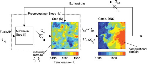
In the combustion DNS (the second stage), the inflowing mixture has pockets of exhaust and fresh gases, and flows at an average velocity of U_in from the inflow boundary located at x = 0 of the computational domain, see Figure 2. The inflowing and initial fields are constructed following the four steps described in the next subsection. The turbulence velocity, mass fractions, and temperature fields at the inflow boundary are specified respectively as:

(8)

(9)

and

(10)

where the quantities with a hat denote the preprocessed fields obtained in the first stage and denotes the x location of a scanning plane at time t moving at a velocity of U_in through the preprocessed fields. In order to contrast the behavior of reaction zones in MILD combustion, a standard turbulent premixed flame is also simulated in this study. This premixed combustion simulation has the same setup, except for the inflowing mass fraction and temperature fields, which are made of homogeneous and uniform unburned gases of the same equivalence ratio as for the MILD cases.

2.3. Construction of Initial and Inflow Fields

The steps involved in the first stage of MILD combustion DNS conducted in this study are described in this subsection.

• Step (i) A turbulent velocity field is generated in a preliminary DNS of freely decaying homogeneous isotropic turbulence inside a periodic cuboid. This flow field is first initialized using a turbulent kinetic energy spectrum (Batchelor and Townsend, 1948) as described by Rogallo (1981). After this initialization, the simulation is continued until the velocity derivative skewness reaches an approximately constant value of −0.5 representing a fully developed turbulence field.

• Step (ii) One-dimensional laminar flames freely propagating into reactant mixtures of a desired MILD condition are calculated using the skeletal mechanism of Smooke and Giovangigli (1991). The reactants for these laminar flames are diluted with products of fully burned mixture , and the mole fraction of O₂ in the reactant mixture is matched to the desired dilution level.

• Step (iii) An initial homogeneous scalar field is obtained by specifying a scalar-energy spectrum function as in Eswaran and Pope (1987). This scalar field is taken as an initial field of a reaction progress variable, defined as taking values between 0 to 1. The same c_Y field is used to initialize all the MILD combustion simulations conducted in this study. The fuel mass fraction is Yf and the subscript, r, denotes reactant mixture. The flame solution from Step (ii) is then mapped to this c_Y field to obtain the spatial variation of Y_α, and the temperature is set to a constant value of T_m to be specified later. The fluctuations in the scalar field obtained in this step do not yet have any correlation with the turbulence field obtained in Step (i). This lack of correlation can lead to some non-physical combustion behavior, which is overcome using the process described in the next step.

• Step (iv) These scalar and turbulence fields are allowed to evolve in the periodic domain to mimic the EGR-mixing without any chemical reaction. This mixing DNS is run for one large eddy turnover time, , which is much shorter than the reference autoignition delay time for the chosen mixture. This allows the correlation between the turbulence and scalar fields to develop. The root-mean-square (RMS) of the turbulent fluctuations obtained in Step (i) is and its integral length scale is . The internal energy equation, Eq. (3), is also solved in this step to mimic the evolution of temperature during the mixing process, which results in a maximum temperature fluctuation of about 2% of a mean value, T_m. This turbulent mixing and the presence of differential diffusion among various species present in the mixture produce fluctuations in the mixture fraction and equivalence ratio fields also, and the RMS values of these fluctuations are about 0.001 and 0.01, respectively.

The spatial variation of the field obtained in Step (iii) is shown in Figure 3a and its probability density function (PDF) is shown in Figure 3b using a gray dashed line. The PDF values are multiplied by 0.1 to fit in the scale shown in this figure. This PDF is bimodal because the mixture composition constructed in Step (iii) uses the laminar flame structure calculated in Step (ii). This field is used to construct the initial and inflowing fields for the three MILD cases investigated in this study and the difference comes only from Step (iv). As noted above, this step mimics the EGR mixing before chemical reactions begin. This mixing process is bound to create samples with ĉ_Y in the range , which is signified by the PDFs shown in Figure 3b for the three cases, Case A1, Case A2, and Case B1, which are described in section 2.4. Also, there are pockets of unburned and burned gases as noted earlier based on physical reasoning. One can also envisage partially premixed conditions containing pockets of pure fuel, air, unburned reactants and burned products. Additional complexities are required to account for this partial premixing during the initialization steps, which is not considered in this study.

Figure 3 (a) Typical spatial variation of field obtained in Step (iii), the field is shown for mid x-y plane. (b) Typical PDF of in the field obtained during the preprocessing. Gray dashed line: initial field obtained in Step (iii), black solid line: preprocessed field obtained in Step (iv) to be used for Case A1, black dashed line: for Case A2, and black dash-dotted line: for Case B1.

Typical spatial variations of the mass fraction fields obtained at the end of Step (iv) are shown in Figure 4. These fields are shown for , , , and for Case B1. Due to intense dilution, is smaller than . As noted earlier, the species fields computed in Step (iv) have evolved with the turbulence resulting in a mixture field containing both well-mixed and partially-mixed pockets of exhaust and fresh gases. Radicals and intermediate species also exist in the domain as shown in Figure 4d. This mixture flows through the inflowing boundary of the computational domain for MILD combustion as per Eqs. (8) to (10).

Figure 4 Typical spatial variation of preprocessed fields of (a) , (b) , (c) , and (d) in mid x-y plane obtained in Step (iv) for Case B1.

The mean and variance of the field obtained at the end of Step (iv) are, respectively, and for all MILD cases considered in this study. The variation of Bilger’s mixture fraction (Bilger et al., 1990) in the preprocessed field is about ±5% of the mean value, . The equivalence ratio obtained using , where is the stoichiometric mixture fraction value, gives a mean value of for all the cases considered in this study. The mixture fraction, , is calculated based on the pure fuel stream and an oxidizer stream of air diluted with products to a desired level of oxygen.

2.4. Turbulent Combustion Conditions

2.4.1. Introduction of MILD flame element

The 1D unstrained laminar flames used in Step (ii) described above for the initial field construction are named as Flames A and B for the MILD cases. The 1D laminar flame used for initial field construction of the premixed case is Flame C. Typical variations of species mass fractions across Flame A are shown in Figure 5a. The distance through this laminar flame is defined using , where is the laminar flame thermal thickness and x_o is the location of peak heat release rate in the laminar flame. The product species mass fractions in the reactant mixture are non-zero due to dilution. The temperature variations in these laminar flames are shown in Figure 5b, and their thermochemical properties are summarized in Table 1. The values of reactant mole fractions, , indicate the level of dilution in the reactant mixture of these laminar flames. The laminar flame speed, , is a few meters per second because of the high reactant temperature, T_r, resulting from preheating. The reference autoignition delay times, , of these diluted mixtures are also given in the table.

Table 1 Summary of laminar flame properties (units are K (Kelvin), meter, and second)

					Tr	Tp	SL
Flame A	0.019	0.048	0.121	0.061	1500	1865	3.20	0.69	5.0
Flame B	0.014	0.035	0.132	0.066	1500	1775	2.15	0.94	6.7
Flame C	0.078	0.194	0.0	0.0	600	2179	1.18	0.37	—
MIFE A	0.0095	0.0349	0.136	0.064	1500	1692	2.62	1.00	5.4
MIFE B	0.0060	0.0248	0.143	0.068	1500	1624	1.66	1.29	7.0

Figure 5 Variations of (a) mass fraction variations of CH₄, O₂, H₂O, CO₂, OH, and CO in Flame A and (b) temperature in one-dimensional laminar flames used for the MILD and premixed combustion cases.

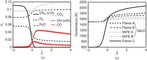
Flame C is a classical premixed flame as indicated by the large temperature rise seen in Figure 5b and the reactant mole fractions listed in Table 1. The temperature rise across the laminar flames with diluted and preheated mixtures is observed to be relatively small, about 370 K for Flame A and 290 K for Flame B. This is typical of MILD combustion. Spatial variations of species mass fraction in the inflowing mixture fields are inevitable, as seen in Figure 4, when the MILD combustion occurs in three dimensions and it is not possible to represent this spatial variation in a representative 1D laminar flame. Indeed, the effect of additional dilution resulting from spatial variation reduces the burned mixture temperature in the turbulent cases by about 150 K compared to the respective laminar flames (Minamoto et al., 2013). To account for this additional dilution effect even for laminar flames, the mass fractions of major species in the reactant mixture are computed based on the volume average of the respective species in the preprocessed DNS initial field obtained in Step (iv) described in section 2.3. A laminar flame having this reactant mixture is named MILD flame element (MIFE) in this study. As one would expect, this averaging yields significantly smaller mole fraction values as noted in Table 1 for MIFEs A and B compared to the Flames A and B. Also, the burned mixture temperature, T_p, is only about 27 K higher than the DNS values (this is the maximum difference observed here). For these reasons, MIFEs are taken to be representative canonical flames (flamelets) for the MILD combustion cases investigated in this study and their thermo-chemical attributes listed in Table 1 are used to normalize the respective DNS results. For example, length, gradient of reaction progress variable, and reaction rate are respectively normalized using and . The quantities normalized are thus denoted using a superscript “+”.

2.4.2. Conditions for turbulent MILD combustion

Three MILD cases and one classical premixed combustion case are simulated directly using the initial and incoming fields generated as described in section 2.3. The turbulence and thermochemical conditions of these four cases are given in Table 2. The thermo-chemical conditions for the Cases A1 and A2 are based on Flame A. Thus, they have the same dilution level, but their turbulence conditions are different as in Table 2. Case A1 has the same turbulence field as in Case B1, but uses the same thermochemical conditions as Case A2. All of the four cases have the same equivalence ratio, , and the au-toignition temperature for this lean methane-air mixture is 1100 K. The temperature of the initial and inflowing mixture is set to be for the MILD combustion cases, and 600 K for the premixed combustion Case C. The high value of T_m for the MILD combustion is comparable to that used by Suzukawa et al. (1997) in their experiments. This inlet temperature together with the low mole fraction of O₂ suggests that the combustion conditions are strictly in the MILD regime as in Figure 1.

Table 2 Conditions of turbulent combustion considered in this study

					Uin/SL	u’/SL				Da	Ka
Case Al	0.048	0.035	0.011	0.014	9.6	6.26	10.8	1.48	96.2 (33)	1.72	4.78
Case A2	0.048	0.035	0.011	0.014	9.6	3.80	12.3	1.70	67.0 (26)	3.25	2.11
Case Bl	0.035	0.025	0.008	0.010	15.1	9.88	6.8	1.15	96.1 (33)	0.69	11.9
Case C	0.194	0.194	0.044	0.055	3.0	2.19	12.3	2.11	38.5 (18)	5.64	0.92

The maximum, and averaged, , mole fractions of oxygen in the reactant mixture for the MILD cases are significantly smaller than for Case C because of the high dilution levels (see Table 2). These dilution levels are comparable with previous studies (Cavaliere and de Joannon, 2004; de Joannon et al., 2000; Katsuki and Hasegawa, 1998).

The mean, , and stoichiometric, , mixture fraction values are also given in Table 2. The RMS of velocity fluctuations and the integral length scale of the initial turbulence field are denoted, respectively, as and l₀ in Table 2. The Zeldovich thickness is , where and c_p are, respectively, the mixture thermal conductivity and specific heat capacity at constant pressure. The Reynolds number, with as the kinematic viscosity of reactant mixture, varies from 67 to 96 for the MILD cases. The values within the bracket denote the Reynolds number based on the Taylor microscale, . An estimate of the Reynolds number for MILD combustion in previous studies (Duwig et al., 2012; Medwell, 2007; Oldenhof et al., 2011) using the information for reacting jet flows (Buschmann et al., 1996; Chen et al., 1996; Duwig et al., 2007; Pfadler et al., 2008) suggests that the values of in Table 2 are comparable to those for previous MILD combustion experiments. The turbulence level for Case C, the premixed combustion case, is deliberately set to be a small value to help contrast the behavior of reaction zones and their structure in MILD conditions and in premixed combustion with a large Damkohler number. The Damköhler and Karlovitz numbers are defined as and , where is the Kol-mogorov length scale. The value of Da and Ka in Table 2 indicates that three MILD cases are in the thin-reaction zones regime, and Case C is near the border between the thin-reaction zones and corrugated flamelets regimes in a turbulent combustion regime diagram (Peters, 2000).

2.4.3. Computational detail

The computational domain is of size for the three MILD cases and for the premixed flame, Case C. If the computational domain is normalized using of the respective laminar flames (MIFEs for MILD and Flame C for premixed cases), for Cases A1 and A2, (7.75)³ for Case B1, and 26.7 × 13.4 x 13.4 for Case C. These domains are discretized using 512 × 512 × 512 mesh points for Cases A1 and A2, 384 × 384 × 384 mesh points for Case B1, and 512 × 256 × 256 mesh points for Case C. These meshes ensure that there are at least 15 mesh points inside the respective thermal thickness .

The simulations of the MILD cases were run for 1.5 flow-through times to ensure that the initial transients had left the domain before collecting data for statistical analysis. The flow-through time is defined as , which is the mean convection time for a disturbance to travel from the inflow to the outflow boundary. The simulations were then continued for one additional flow-through time and 80 data sets were collected. For Case C, 93 data sets were collected over a time of 0.56 after allowing one flow-through time for initial transients to exit the computational domain. These simulations have been run on Cray XE6 systems using 4096 cores with a wall-clock time of about 120 h for Case A1 and Case A2, which have the largest number of mesh points, and using 16,384 cores with 80 h of wall-clock time for Case C.

3. RESULTS AND DISCUSSION

3.1. Temperature Field in MILD Combustion

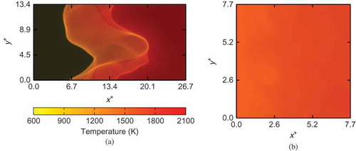
Volume rendered images of the temperature field for MILD (Case B1) and premixed combustion (Case C) cases are shown in Figure 6. These snapshots are taken at t = 1.5 looking through the z-direction, and the color map used is the same for both cases. Hence, these figures can be compared directly as is often done in experiments using direct photographs of flames. There are no visible flames or high gradient fronts in the MILD combustion case shown in Figure 6b unlike the premixed case in Figure 6a where flame fronts are apparent. These results show that the MILD combustion considered in the present study indeed has a relatively uniform temperature field compared to the premixed case, and such an observation is similar to those observed in the previous experimental studies (de Joan-non et al., 2000; Krishnamurthy et al., 2009; Özdemir and Peters, 2001).

Figure 6 Comparison of typical volume rendered temperature field in (a) premixed case and (b) MILD combustion, Case B1.

The PDF of a reaction progress variable, , is shown in Figure 7 for the same cases as in Figure 6. The results are shown for different streamwise locations across the computational domain. These PDFs are constructed using samples from the entire sampling period. The PDFs for Case C in Figure 7a show typical behavior of the progress variable in premixed combustion. The locations x⁺ = 7.48, 17.5, and 25.9 correspond respectively to upstream, inside, and downstream positions of the flame brush. These PDFs have sharp peaks at c_T ∼ 0 and close to c_T ∼ 1, and the probability of finding intermediate values is very small for all the locations shown in this figure, which results from combustion in thin reaction zones with a strong scalar gradient as observed in Figure 6a. Specifically, the PDF at x⁺ = 17.5 shows a bimodal distribution of c_T, which peaks at c_T ∼ 0 and 0.92. The PDF peak does not occur at c_T ∼ 1 because of the use of multi-step chemistry (finite rate chemistry) and the finite size of the computational domain. A much longer domain is needed to observe the equilibrium temperature of the product, T_p.

Figure 7 Typical PDF of reaction progress variable based on temperature at various x⁺ locations for (a) Case C and (b) Case B1.

The PDFs of c_T for the MILD case, however, show neither sharp peaks nor bimodality for the locations depicted in Figure 7b. The PDF for a location near the inlet boundary, x⁺ = 0.30, has a relatively sharp peak at about c_T = 0.05, showing that unburned gases are predominant at this location. This peak shifts towards c_T =1 as one moves in the downstream direction, after reaching a plateau covering the range 0.2 ≤ c_T ≤ 0.7 for the location x⁺ = 2.9. This plateau suggests distributed combustion, although this could also be due to thickening of the reaction zones despite the overall combustion conditions being in the thin reaction zones regime. The physics behind this thickening is different from that for classical thin reaction zones regime combustion where the small-scale turbulent eddies enter the preheat zone and broaden this zone. The physical processes responsible for the thickening of the reaction zones in the MILD combustion are discussed in the following section.

3.2. Reaction Zone Behavior

The iso-surfaces of normalized reaction rate of c_T calculated as using the heat release rate are shown in Figure 8 for the same cases as in Figures 6 and 7. The regions with intense reaction rate are bounded by two iso-surfaces of for the premixed case as in Figure 8a. This is typical of turbulent premixed combustion in the thin reaction zones regime involving high Da and low Ka numbers. Such reaction zone behavior makes it possible to use flamelet type modeling (Peters, 2000).

Figure 8 Typical iso-surface of reaction rate at . (a) for the premixed case and (b) for Case B1. Note that only of the computational domain is shown for Case C in (a).

The reaction rate iso-surface shown in Figure 8b for the Case B1 suggests that chemical reactions occur over a larger region in MILD combustion unlike in the premixed case. The reaction rate is not uniform and homogeneous in space as one may expect to see based on the volume rendered image shown in Figure 6b, which is similar to a direct photograph from MILD combustion experiments. These reaction zones are highly convoluted with a strong possibility for interaction between them. The high iso-surface density near the inflow boundary observed in Figure 8b suggests that the MILD mixture reacts as soon as it enters the domain due to its elevated temperature. The iso-surfaces become more sparse towards the outflow boundary because of non-availability of fuel for further reaction.

To develop further understanding of the reaction zone behavior in MILD combustion, 2D slices of in a mid x-y plane are plotted in Figure 9 using DNS data at . The premixed case is shown in Figure 9a and Cases A1, A2, and B1 of the MILD combustion are shown, respectively, in Figures 9b, 9c, and 9d. For the premixed case, the reaction zone is thin having a typical thickness of about as in Figure 9a, suggesting typical flamelet-like thin reaction zones. Also, the intense reaction occurs along an iso-surface of c_T = 0.6, which is also bounded well by the c_T = 0.2 and 0.8 iso-surfaces as in Figure 9a. This behavior is well known for turbulent combustion in the thin reaction zones regime.

Figure 9 Variations of (color) and c_T (lines) in the mid x-y planes for (a) Case C, (b) Case A1, (c) Case A2, and (d) Case B1. Dash-dotted line: , solid line: , and dashed line: . Note that only of the computational domain is shown for Case C in (a). Snapshots are taken at .

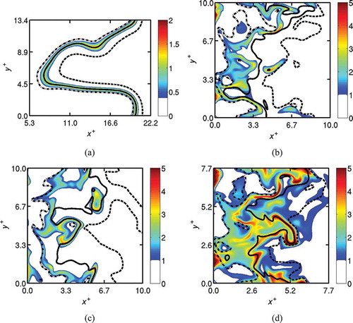
Interactions between the reaction zones are observed in the 2D slices shown for the MILD cases in Figures 9b to 9d. The reaction zone thickness in the interacting regions have a typical thickness of about to , while it is about δ_th for non-interacting regions. The reaction rate contours shown in Figure 9 suggest that regions of intense reactions occupy a substantial volume in upstream regions (x < 0.5L_x) for the MILD cases. The volume occupied by intense chemical activity seems to decrease with streamwise distance for Cases A1 and A2. However, Figure 9d shows that the highly convoluted reaction zones in Case B1 reach the outflow boundary, and interactions occur more often (see Figure 10) for Case B1 compared to the other MILD cases.

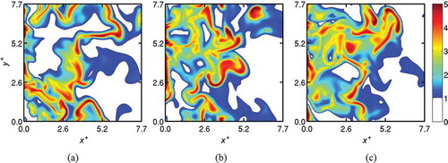
Figure 10 Spatial variation of in the mid x-y plane for Case B1 at (a) , (b) , and (c) .

A comparison of Case C and Case A2, shown respectively in Figures 9a and 9c, suggests that the MILD reaction zones are highly convoluted despite the similar values of , , and Da and Ka numbers for these two cases (see Table 2). This suggests that the reaction zone convolutions observed for the MILD cases are not caused solely by turbulence-chemistry interactions. The effects of mixture dilution leading to spatially non-uniform combustion play a predominant role and this becomes clearer if one compares Cases A1 and A2 shown in Figures 9b and 9c, respectively. These two cases have the same dilution level but different turbulence conditions as noted in Table 2, and the degree of convolution of their reaction zones observed in Figure 9 are similar. It is worth noting that the value of is about 65% larger and the value of is about 12% smaller for Case A1 compared to Case A2.

The dilution level does not only affect the thermo-chemical condition but also the turbulence-chemistry interaction because of a change in the relative time and length scales between turbulence and chemistry (compare Da and Ka values for Case A1 and Case B1). Thus, there are compounding effects leading to dramatic changes in reaction zone behavior when the dilution level is changed. This is seen clearly if one compares Figures 9b and 9d in relation to the above observation for Cases A1 and A2. Cases B and A1 use the same turbulence field as noted in section 2.4.2, but the dilution level for Case B1 is larger than that of Case A1, resulting in the value being 58% larger and the value being 37% smaller for Case B1 compared to Case A1. These changes alter the Da and Ka number significantly by an order of magnitude although Re_lo is the same, and thus the turbulence-chemistry interaction is expected to be quite different (Peters, 2000; Swaminathan and Bray, 2005). For these reasons, one observes a high level of reaction zone convolution in Case B1 as shown in Figure 9d.

The contours of are also shown in Figure 9 to convey another important observation for MILD combustion. Unlike classical premixed combustion, the peak reaction rate does not occur always for a particular value and the contours of are not always parallel to one another. This behavior observed in the present MILD cases is suggestive of non-flamelet combustion with reaction zones spread out over a large portion of the volume. Also, the local presence of thin reaction zones or flamelets is clearly observed. This non-flamelet behavior of the iso-contours and reaction zones results from the interaction of reaction zones as has been observed in an earlier study (Minamoto and Swaminathan, 2014; Minamoto et al., 2013).

Figure 10 shows the reaction rate contours for Case B1 in the mid x-y plane for three different times, , 2.0, and 2.25, to investigate the temporal variation of reaction zone behavior. The behavior seen in this figure is very similar to that observed in Figure 9d. Thus, the interaction of reaction zones or flamelets must be included if one wishes to use flamelet-based models for turbulent MILD combustion. This requirement is expected to become more important at high dilution levels of practical interest.

To shed more light on the different behavior between temperature and OH fields reported in previous experiments (Dally et al., 2004; Duwig et al., 2012; Özdemir and Peters, 2001; Plessing et al., 1998) as described in the introduction, the spatial variations of normalized temperature, , and OH mass fraction are shown in Figure 11 as contours. The subscripts “max” and “min” denote, respectively, the maximum and minimum values in the respective 2D slices and thus T* and c_T are almost identical, but not exactly the same. Similar comparisons using laser thermometry and OH-PLIF images have been reported in previous experimental studies (Dally et al., 2004; Duwig et al., 2012; Özdemir and Peters, 2001; Plessing et al., 1998).

Figure 11 Typical spatial variations of the normalized temperature, T* (shown in a and c) and (b and d) for Case B1. The contours are shown for the mid x-y plane (a and b), and y-z plane at x = L_x/3 (c and d) at . The contour levels are 0.2 (dash-dotted line), 0.4 (continuous lines), and 0.6 (dashed lines).

The temperature increase is relatively gradual suggesting distributed reaction zones, while the OH field exhibits thin reaction zones with a strong gradient (compare the distance between dash-dotted and dashed lines in Figure 11) in substantial regions. A similar comparison is observed in previous experiments (Dally et al., 2004; Duwig et al., 2012; Özdemir and Peters, 2001; Plessing et al., 1998). Also, the DNS results suggest a patchy appearance of reaction zones, which was also reported by Dally et al. (2004). The difference of these two fields is due to the effects of non-unity Lewis numbers and complex chemical kinetics. These features cannot be reproduced if single step chemistry was used for the DNS. To gain further understanding of the behavior of these reaction zones, their structures are studied in the next subsection by investigating the variations of species mass fractions and reaction rate with temperature.

3.3. Reaction Zone Structure in MILD Combustion

Typical variations of species mass fractions with temperature in the MILD Cases A1 and B1 are shown in Figure 12 as scatter plots. The conditional average mass fractions constructed using the samples collected over the entire sampling period are also shown in Figure 12. Furthermore, the results of the laminar Flames A and B, and MIFEs are also included for comparison purposes. These conditional averages are very close to and the temperature is used here for conditioning following a common practice in laser diagnostics of premixed combustion.

Figure 12 Variation of species mass fractions, CH₄ (a, d), H₂O (b, e), and OH (c, f), with temperature in the MILD combustion DNS (scatter), Case A1 (a–c) and Case B1 (d–f). Continuous line: the conditional average of the DNS results; dashed line: the respective laminar flames in Table 1, and dash-dotted line: the respective MIFE in Table 1. The data for scatter plot is taken at and conditional average is calculated using data from the entire sampling period.

There is a large scatter in for lower temperature because of inhomogeneity in the inflowing mixture containing pockets of exhaust and fresh mixtures. This large scatter is consistent with the field shown in Figure 4 for Case B1. The scatter in reduces as the temperature increases, because of the combined effects of combustion, molecular diffusion, and turbulent mixing. This mixing process reduces the inhomogeneity in the mixture leading to reduced scatter as T increases.

As noted in section 2.3, the reactant mixtures for Flames A and B do not include the effect of additional dilution due to exhaust gas pockets, and the oxygen mole fraction is larger than the average value in the respective DNS cases (compare Tables 1 and 2). Thus, the product temperature in these laminar flames is larger than that in the respective DNS as noted in section 2.4.1. Also, a comparison between Flames A and B solutions and the conditional average shows that the variations of mass fractions with T in Flames A and B are not representative of the variations in the MILD combustion DNS. In contrast, MIFEs seem to be representative of the MILD reaction zones structure at least for major species (not all of them are shown here). The poor agreement seen for the minor species such as OH is because the reactant mixture for the MIFEs excludes intermediate species, which are present in the initial inhomogeneous mixture for the DNS. However, the agreement for minor species in Figure 12 is improved for MIFEs compared to Flames A and B. This is because the additional dilution effect is included in the reactant mixture of the MIFEs as explained in section 2.4.1.

Figure 13 shows the variation of , with for the three MILD cases considered in this study. The results for the classical premixed case, Case C, are also included for comparison. The data for the scatter plots is taken at , and the conditionally averaged values are constructed using samples collected over the entire sampling period as has been done for Figure 12. The maximum value of observed over the entire sampling period for a given is also shown in Figure 13. The scatter in , for the premixed case is smaller compared to the MILD cases and has a peak at ≈ 0.6. The conditionally averaged reaction rate suggests that the peak reaction rate occurs at smaller in the MILD cases compared to the premixed case. This behavior of is because the temperature rise in MILD combustion is gradual due to heat conduction to non-burning regions containing relatively cooler products.

Figure 13 Variation of with in (a) Case A1, (b) Case A2, and (c) Case B1. The scatter with light gray points is for MILD combustion and the dark gray points are for the premixed case. The points are taken at t = 1.5τ_D, and the thin dashed line is the maximum value observed in the DNS from the entire sampling period. Solid line: the conditional average , and dash-dotted line: the respective MIFE.

The solution for the respective MIFE is also shown using a dash-dotted line in Figure 13 and the results of Flame A and B are not shown, since they deviate significantly from the DNS and MIFE results as discussed in Figure 12. Although the trends in the variations of with are similar to the DNS results, the quantitative agreement is not as good as that for the major species mass fractions shown in Figure 12. The peak value of in the MILD case is higher than the respective MIFE values. The difference between the peak values in the DNS and the respective MIFE solution increases with increasing dilution and turbulence levels as shown in Figure 13: 0.54 for Case A1, 0.41 for Case A2, and 1.66 for Case B1. Also, there is a substantial reaction rate in the DNS for = 0 as indicated by the conditional reaction rate, and this is not captured in the MIFE result. The reduced reaction rate in the MIFE is because its solution does not fully account for the effects of exhaust gas pockets present in the initial/inflowing mixtures. Specifically, the presence of radicals is not captured. Also, a MIFE has a thin propagating reaction zone as in a classical laminar premixed flamelet. As the dilution level increases in the MILD combustion, the presence of individual reaction zones influenced only by turbulence-chemistry interaction becomes less clear due to the interaction of reaction zones as noted in section 3.2. Thus, a fully representative canonical reactor for turbulent MILD combustion needs to include effects of locally homogeneous combustion resulting from interactions and collisions of reaction zones and, classical combustion in thin reaction zones creating spatial gradients.

4. Summary and conclusions

Three-dimensional DNS of turbulent MILD and premixed combustion has been conducted to investigate the behavior of reaction zones and their structure in MILD combustion. The results of the premixed case are used for comparative analyses. A fully compressible formulation with temperature-dependent transport properties is used for the DNS, and the combustion kinetics are simulated using a skeletal mechanism for methane-air combustion. The DNS configuration includes inflow, non-reflecting outflow, and periodic boundaries, and the inflow mixture contains pockets of unburned and burned gases to be representative of MILD combustion with exhaust gas recirculation. A methodology to construct a consistent turbulence and non-uniform mixture field is described in detail.

Often, MILD combustion is called “flameless” combustion implying that it does not involve flames or thin reaction zones. The analysis of DNS data clearly showed that there are regions with strong chemical activity (flamelets) and these regions are distributed over a good portion of the computational domain, unlike in the premixed flame having reaction zones confined to a small portion of the computational domain. Also, interactions of reaction zones are observed in MILD combustion. The frequency and spatial extent of this interaction increase with dilution and turbulence levels. Such interactions yield an appearance of distributed reaction zones and result in a relatively uniform temperature distribution, which is also observed in the volume rendered temperature field. This effect produces mono-modal PDFs for the reaction progress variable in MILD combustion as opposed to a standard bi-modal PDF for turbulent premixed combustion.

Scatter plots of instantaneous species mass fraction and reaction rate show a wide scatter due to mixture inhomogeneity for MILD combustion. The conditionally averaged mass fractions are also analyzed to see whether a canonical laminar flame can be used to represent the MILD reaction zones. The canonical flame, called MIFE (MILD flame element), is introduced for this purpose, and it has diluted reactants made of unburned and burned mixtures, containing only major species. A comparison of averaged species mass fractions conditioned on temperature between the MILD combustion DNS and the MIFE values suggests that the MIFE is a reasonable candidate for major species. However, similar comparisons for minor species and reaction rates are less satisfactory. Thus, an alternative canonical combustion model, which can include effects of non-flamelet combustion resulting from interaction of reaction zones and still cater for flamelet combustion, needs to be developed for MILD combustion.

FUNDING

YM acknowledges the financial support of Nippon Keidanren and Cambridge Overseas Trust. EPSRC support is acknowledged by NS. The support of the Natural Sciences and Engineering Research Council of Canada is acknowledged by TL. This work made use of the facilities of HECToR, the UK’s national high-performance computing service, which is provided by UoE HPCx Ltd at the University of Edinburgh, Cray Inc, and NAG Ltd, and funded by the Office of Science and Technology through EPSRC’s High End Computing Programme.

REFERENCES

- Awosope, I., Kandamby, N., and Lockwood, F. 2006. Flameless oxidation modelling: On application to gas turbine combustors. J. Energy Inst., 79, 75–83.
- Batchelor, G.K., and Townsend, A.A. 1948. Decay of turbulence in the final period. Proc. R. Soc. Lond, A, 194( 1039), 527–543.
- Bilger, R.W., Stårner, S.H., and Kee, R.J. 1990. On reduced mechanism for methane-air combustion in nonpremixed flames. Combust. Flame, 80, 135–149.
- Buschmann, A., Dinkelacker, F., Schäfer, T., and Wolfrum, J. 1996. Measurement of the instantaneous detailed flame structure in turbulent premixed combustion. Proc. Combust. Inst., 26(1), 437–445.
- Cant, R. S. 2012. SENGA2 User Guide. Technical Report CUED/A–THERMO/TR67. Cambridge University Engineering Department.
- Cavaliere, A., and de Joannon, M. 2004. Mild combustion. Prog. Energy Combust. Sci., 30, 329–366.
- Chen, J.H. 2011. Petascale direct numerical simulation of turbulent combustion fundamental insights towards predictive models. Proc. Combust. Inst., 33, 99–123.
- Chen, Y.C., Peters, N., Schneemann, G.A., Wruck, N., Renz, U., and Man-sour, M.S. 1996. The detailed flame structure of highly stretched turbulent premixed methane-air flames. Combust. Flame, 107, 223–244.
- Coelho, P. J., and Peters, N. 2001. Numerical simulation of a MILD combustion burner. Combust. Flame, 124, 503–518.
- Dally, B.B., Karpetis, A.N., and Barlow, R.S. 2002. Structure of turbulent nonpremixed jet flames in a diluted hot coflow. Proc. Combust. Inst., 29, 1147–1154.
- Dally, B.B., Riesmeier, E., and Peters, N. 2004. Effect of fuel mixture on moderate and intense low oxygen dilution combustion. Combust. Flame, 137, 418–431.
- Dunstan, T.D., Swaminathan, N., and Bray, K.N.C. 2012. Influence of flame geometry on turbulent premixed flame propagation: A DNS investigation. J. Fluid Mech., 709, 191–222.
- Dunstan, T.D., Swaminathan, N., Bray, K.N.C., and Cant, R.S. 2011. Geometrical properties and turbulent flame speed measurements in stationary V-flames using direct numerical simulation. Flow Turbulence Combust., 87, 237–259.
- Duwig, C., Fuchs, L., Griebel, P., Siewert, P., and Boschek, E. 2007. Study of a confined turbulent jet: Influence of combustion and pressure. AIAA J., 45(3), 624–639.
- Duwig, C., Li, B., and Aldén, M. 2012. High resolution imaging of flameless and distributed turbulent combustion. Combust. Flame, 159, 306–316.
- Duwig, C., Stankovic, D., Fuchs, L., Li, G., and Gutmark, E. 2008. Experimental and numerical study of flameless combustion in a model gas turbine combustor. Combust. Sci. Technol., 180(2), 279–295.
- Eswaran, V., and Pope, S. B. 1987. Direct numerical simulations of the turbulent mixing of a passive scalar. Phys. Fluids, 31(3), 506–520.
- Galleti, C., Parente, A., and Tognotti, L. 2007. Numerical and experimental investigation of a Mild combustor burner. Combust. Flame, 151, 649–664.
- Hayashi, S., and Mizobuchi, Y. 2011. Utilization of hot burnt gas for better control of combustion and emissions. In N. Swaminathan and K. N. C. Bray (Eds.), Turbulent Premixed Flames, Cambridge University Press, Cambridge, UK, pp. 365–378.
- De Joannon, M., Saponaro, A., and Cavaliere, A. 2000. Zero-dimensional analysis of diluted oxidation of methane in rich conditions. Proc. Combust. Inst., 28, 1639–1646.
- Katsuki, M., and Hasegawa, T. 1998. The science and technology of combustion in highly preheated air. Proc. Combust. Inst., 27(2), 3135–3146.
- Krishnamurthy, N., Paul, P. J., and Blasiak, W. 2009. Studies on low-intensity oxy-fuel burner. Proc. Combust. Inst., 32, 3139–3146.
- Li, P., and Mi, J. 2011. Influence of inlet dilution of reactants on premixed combustion in a recuperative furnace. Flow Turbulence Combust., 87(4), 617–638.
- Medwell, P.R. 2007. Laser diagnostics in MILD combustion. PhD thesis, The University of Adelaide, Adelaide, Australia.
- Minamoto, Y., Dunstan, T.D., Swaminathan, N., and Cant, R.S. 2013. DNS of EGR-type turbulent flame in MILD condition. Proc. Combust. Inst., 34, 3231–3238.
- Minamoto, Y., and Swaminathan, N. 2014. Scalar gradient behaviour in MILD combustion. Combust. Flame, 161, 1063–1075.
- Mohamed, H., Bentîcha, H., and Mohamed, S. 2009. Numerical modeling of the effects of fuel dilution and strain rate on reaction zone structure and NOx formation in flameless combustion. Combust. Sci. Technol., 181(8), 1078–1091.
- Van Oijen, J. A. 2013. Direct numerical simulation of autoigniting mixing layers in MILD combustion. Proc. Combust. Inst., 34(1), 1163–1171.
- Oldenhof, E., Tummers, M.J., Van Veen, E.H., and Roekaerts, D.J.E.M. 2011. Role of entrainment in the stabilisation of jet-in-hot-coflow flames. Combust. Flame, 158, 1553–1563.
- Özdemir, Í.B., and Peters, N. 2001. Characteristics of the reaction zone in a combustor operating at MILD combustion. Exp. Fluids, 30, 683–695.
- Peters, N. 2000. Turbulent Combustion, Cambridge University Press, Cambridge, UK.
- Pfadler, S., Leipertz, A., and Dinkelacker, F. 2008. Systematic experiments on turbulent premixed Bunsen flame including turbulent flux measurement. Combust. Flame, 152, 616–631.
- Plessing, T., Peters, N., and Wünning, J.G. 1998. Laseroptical investigation of highly preheated combustion with strong exhaust gas recirculation. Proc. Combust. Inst., 27, 3197–3204.
- Poinsot, T., and Lele, S. 1992. Boundary conditions for direct simulations of compressible viscous flows. J. Comput. Phys., 101, 104–129.
- Rogallo, R.S. 1981. Numerical experiments in homogeneous turbulence. NASA Technical Memorandum 81315.
- Smooke, M.D., and Giovangigli, V. 1991. Formulation of the premixed and non-premixed test problems. In M. D. Smooke (Ed.), Reduced Kinetic Mechanisms and Asymptotic Approximations for Methane-Air Flames., Vol. 384, Springer Verlag, New York, pp. 1–28.
- Suzukawa, Y., Sugiyama, S., Hino, Y., Ishioka, M., and Mori, I. 1997. Heat transfer improvement and NOx reduction by highly preheated air combustion. Energy Convers. Manage., 38(10–13), 1061–1071.
- Swaminathan, N., and Bray, K.N.C. 2005. Effect of dilatation on scalar dissipation in turbulent premixed flames. Combust. Flame, 143, 549–565.
- Woelk, G., and Wünning, J. 1993. Controlled combustion by flameless oxidation. Joint Meeting of the British and German Sections of the Combustion Institute, Cambridge, UK.
- Wünning, J.A. 1991. Flameless oxidation with highly preheated air. Chem. Ing. Tech., 63(12), 1243–1245.
- Wünning, J.A., and Wünning, J.G. 1997. Flameless oxidation to reduce thermal NO-formation. Prog. Energy Combust. Sci., 23, 81–94.