Direct Numerical Simulation of Complex Fuel Combustion with Detailed Chemistry: Physical Insight and Mean Reaction Rate Modeling

Abstract

Direct numerical simulation (DNS) of freely-propagating premixed flames of a multi-component fuel is performed using a skeletal chemical mechanism with 49 reactions and 15 species. The fuel consists of CO, H₂, H₂O, CH₄, and CO₂ in proportions akin to blast furnace gas or a low calorific value syngas. The simulations include low and high turbulence levels to elucidate the effect of turbulence on realistic chemistry flames. The multi-component fuel flame is found to have a more complex structure than most common flames, with individual species’ reaction zones not necessarily overlapping with each other and with a wide heat releasing zone. The species mass fractions and heat release rate show significant scatter, with their conditional average however remaining close to the laminar flame result. Probability density functions of displacement speed, stretch rate, and curvature are near-Gaussian. Five different mean reaction rate closures are evaluated in the RANS context using these DNS data, presenting perhaps the most stringent test to date of the combustion models. Significant quantitative differences are observed in the performance of the models tested, especially for the higher turbulence level case.

Keywords:

• Combustion modeling
• Detailed chemistry
• Direct numerical simulation
• Multi-component
• RANS

INTRODUCTION

Direct numerical simulation (DNS) of turbulent premixed flames is of paramount importance for developing combustion sub-models for RANS and LES computations of practical reacting flows. A key issue in reacting flow DNS is the chemical kinetics modeling. A good representation of combustion kinetics requires the use of complex chemical mechanisms involving more than 100 reactions and 50 species. This level of chemical detail coupled to the 3D nature of turbulent flows, demand prohibitively expensive computational resources. However, DNS with skeletal mechanisms, although still expensive, provides a compromise between the conflicting demands of chemical detail and computational expense. Skeletal chemistry provides more accurate information than 1-step or reduced chemistry models, thus enabling more accurate combustion sub-model development. The first study using a skeletal mechanism was over 15 years ago (Baum et al., 1992, 1994a), investigating premixed hydrogen-air combustion in 2D turbulence. It was concluded that the flame structure correlated more with tangential strain rate than curvature when more realistic chemistry and transport models are used. This observation was employed in subsequent combustion model development.

Since then, there have been many DNS studies of premixed combustion employing skeletal chemistry to examine the role of chemical mechanism, turbulence level, equivalence ratio, and flow configuration. These studies were predominantly for 2D turbulent combustion of hydrogen air (Baum et al., 1992, 1994; Chen and Im, 2000; Im and Chen, 2002; Lange et al., 1998) and methane-air (Chen et al., 1999; Domingo et al., 2005; Echekki and Chen, 1999; Gran et al., 1996; Hawkes and Chen, 2004, 2006; Kaminski et al., 2000; Peters et al., 1998) mixtures. There were some 3D direct simulations of premixed hydrogen (Hawkes et al., 2012; Tanahashi et al., 1999, 2002; Tanaka et al., 2011) and methane (Bell et al., 2002; Sankaran et al., 2006; Thévenin et al., 2002) combustion. Non-premixed combustion of a hydrogen jet issuing into still air has also been simulated in 3D (Mizobuchi et al., 2002, 2005).

Direct simulation of combustion of other fuels of future interest, such as syngas involving a multi-component fuel, has rarely been done except a case of non-premixed combustion of a CO/H₂-air mixture (Hawkes et al., 2007). Understanding turbulent combustion of such alternative fuels is very important, especially in the current energy climate. Such future fuels will probably be multi-component, with a composition specifically designed to minimize environmental impact and to conserve our natural resources. Fuels, such as synthetic gas (syngas), blast furnace gas (BFG), and coke oven gas (COG) are already being used for power generation in industrial gas turbines (Komori et al., 2004). All of these gases are multi-component fuels with CO, H₂, H₂O, CH₄, CO₂, O₂, and N₂ as major components. Furthermore, the relative proportions of these species can vary a lot depending on their production process (Maustard, 2005). In addition, there are species with widely differing thermo-physical and thermo-chemical characteristics. The H₂O can alter the chemical pathway depending on its concentration and it can enhance combustion by supplying OH radicals (Das et al., 2011; Nikolaou et al., 2013; Singh et al., 2012). The CO₂ mainly increases the specific heat capacity of the mixture, thus reducing the flame temperature and speed. H₂ can enhance combustion through preferential diffusion effects when it is in large amounts (Hawkes et al., 2012). All of these effects play key roles in determining the flame response to turbulence. Despite this fact, most combustion sub-models currently employed for practical reacting flow calculations were developed based on DNS of simple fuels, as noted earlier. Thus, there is a need to directly simulate turbulent combustion of multi-component fuels.

The objectives of this study are: (1) to conduct 3D DNS of multi-component fuel combustion using a suitable skeletal mechanism, (2) to analyze the flame front structure and its response to turbulence, and (3) to examine whether this combustion can be modeled using some common mean reaction rate closures.

The remaining of this article is organized as follows: the mathematical background and the numerical implementation are presented next, followed by a discussion of the results, and conclusions are drawn in the final section.

MATHEMATICAL BACKGROUND

Governing Equations and Numerical Method

Direct numerical simulations are conducted using the SENGA2 code (Cant, 2012), which solves fully compressible conservation equations for mass, momentum, energy, and mass fraction of species α. These equations are written, respectively, as:

(1)

(2)

(3)

(4)

using standard notations. The mixture thermal equation of state is , where R⁰ is the universal gas constant, T is the absolute temperature, and is the molecular weight of a species α. The total energy per unit mass, E, is defined as , where the species enthalpy is:

(5)

In Eq. (5), is the constant pressure specific heat capacity of the species, and is its enthalpy of formation at a reference temperature, T₀.

The viscous stress tensor is given by and the heat flux vector is , where is the species diffusion velocity in direction k, and is modeled using a mixture-average diffusivity formulation using the species Lewis number. The standard closure for the mixture’s thermal conductivity is used (Smooke and Giovangigli, 1991). The mixture’s dynamic viscosity, μ, is obtained using , where Pr = 0.7 is the mixture’s Prandtl number, which is taken as a constant from unstrained laminar flame calculations. The species Lewis numbers are calculated by taking the average Lewis number for each species across a freely propagating laminar premixed flame, and these values are given in Table 1. The chemical kinetics are modeled using the chemical mechanism of Nikolaou et al. (2013) involving 49 reactions and 15 species. Further details of the numerical implementation can be found in the SENGA2 user manual (Cant, 2012).

Table 1 Species Lewis numbers

Index	Species	Le
1	H	0.156
2	O2	0.996
3	H2O	0.756
4	CO	0.991
5	CO2	1.311
6	H2	0.264
7	H2O2	1.005
8	OH	0.650
9	HO2	0.998
10	HCO	1.149
11	O	0.637
12	CH4	0.896
13	CH3	0.891
14	CH2O	1.159
15	N2	0.922

Flow Configuration and Boundary Conditions

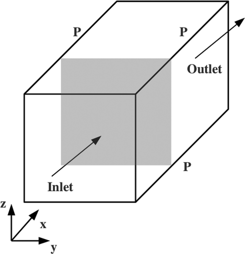
A schematic of the computational domain used to simulate a freely propagating turbulent premixed flame of a multi-component fuel-air mixture is shown in Figure 1. Periodic boundary conditions are applied in the homogeneous (y, z) directions. The inflow boundary at x = 0 has constant density reflecting inflow conditions, and the outflow boundary is partially reflecting based on characteristics analysis (Thompson, 1987, 1990), which was later extended to the NSCBC formulation for single and multi-component mixtures (Baum et al., 1994; Poinsot and Lele, 1992; Sutherland and Kennedy, 2003). Transverse convective terms are included (Yoo et al., 2005; Yoo and Im, 2007) at the inflow and outflow boundaries to ensure numerical stability.

Figure 1 Schematic of the computational domain. Gray area indicates laminar flame used for initialization.

At the inlet , where is a constant mean inlet velocity and is the turbulent velocity fluctuations. These fluctuations are obtained from a non-reacting run of homogeneous isotropic decaying turbulence starting from a Batchelor–Townsend energy spectrum inside a periodic box. This pre-computed field is added to at the inlet for every time step. A scanning plane runs through the pre-computed velocity field and Fourier interpolation is used to correctly update the inlet boundary. The inflowing turbulence is homogeneous and isotropic and it decays downstream. The root-mean-square (rms) value of these velocity fluctuations, , and its integral length scale, , only serve to characterize the turbulence at the inlet. The turbulent kinetic energy dissipation rate is high at the inlet and so the initial laminar flame interacts with a relatively weaker turbulence than at the inlet. This cannot be avoided in simulations of this kind (Sankaran et al., 2006; Tanaka et al., 2011; Tanahashi et al., 1999; Thévenin et al., 2002), unless the turbulence Reynolds number, , where is the kinematic viscosity of reactant mixture, is sufficiently low or turbulence is forced and these approaches have their own disadvantages.

Mixture Conditions

The scalar field is initialized using steady-state laminar flame solutions obtained using the PREMIX code of the CHEMKIN package (Kee et al., 1985, 1992). The fuel mixture is at T_r = 800 K, 1 atm and has an equivalence ratio of . This mixture is composed of CO, H₂, H₂O, CO₂, and CH₄, and the mole fraction of these species are given in Table 2. This composition is typical of a BFG mixture or a low-hydrogen content syngas (Komori et al., 2004). At these conditions, the laminar flame speed is and the laminar flame thermal thickness is , where and T_p is the product temperature.

Table 2 Fuel mixture composition (molar percentages) used in the DNS

Tr (K)		p (atm)	CO	H2	H2O	CO2	CH4	δ (mm)	δl (mm)	δql (mm)	sl (m/s)
800.0	1.0	1.0	62.687	1.881	16.000	18.806	0.627	0.033	0.75	10.8	2.47

Note. The oxidizer is atmospheric air.

Turbulent Flame Conditions

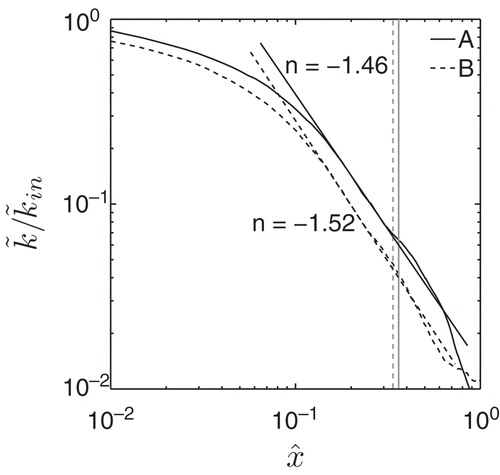
The turbulence and thermo-chemical parameters for the DNS are listed in Table 3. The Damkohler number is defined as and the Karlovitz number is defined as , where is the Kolmogorov length scale and is the Zeldovich thickness. Since the inflowing homogeneous isotropic turbulence decays before encountering the flame, these parameters’ values near the leading side of the flame-brush are also given in Table 3. To have some understanding of the spatial decay, Favre-averaged turbulent kinetic energy, , variation with distance , normalized by the computational domain length, L_x, in the x direction, is shown in Figure 2, for the two cases A and B. The turbulent kinetic energy is normalized by its value at the inlet boundary, and the Favre-averaging used here is explained later in the Post-Processing Method section. The leading flame front locations in the two cases corresponding to , are also marked in Figure 2. Although the flame-brush introduces anisotropy and inhomogeneity, the decay of follows a power law with an exponent of for case A and for case B. These values of n are close to experimental values observed for (non-reacting) grid turbulence (Comte-Bellot and Corrsin, 1966). This occurs up to about , after which the linear relation is somewhat distorted due to flow dilatation as a result of the heat release.

Table 3 Turbulent flame parameters for the DNS at the inlet and at the leading flame front ()

Case	urms/sl	lint/δ	Ret	Da	Ka
A, inlet	3.18	16.54	52.66	5.19	1.39	2.6	9.76	33.92
	0.76	17.41	13.25	22.85	0.16	—	—	—
B, inlet	14.04	16.43	230.69	1.17	12.97	4.8	4.05	80.06
	2.87	36.81	105.61	12.82	0.80	—	—	—

Note. The total run time of the simulations is t_total.

Figure 2 The variation of normalized with . The mean leading flame front position is marked using vertical lines corresponding to in the respective cases.

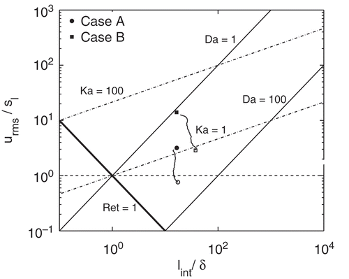
Figure 3 shows the locations of turbulent combustion conditions in the combustion regime diagram (Peters, 2000). The closed symbols correspond to the inlet turbulence conditions and open symbols are for turbulence conditions near the flame-brush leading edge. Also shown is the trajectory from inlet to the location of . The values of Da increase by a factor 4 in case A and by an order of magnitude in case B as noted in Table 3. The changes in Ka values are by orders of magnitude. The simulations are run for 9.76 and 4.05 flame times, , which correspond to 33.92 and 80.06 eddy turn-over times , for cases A and B, respectively.

Figure 3 The combustion regime diagram showing conditions of DNS flames. Filled symbols show conditions corresponding to inlet turbulence parameters, and open symbols show conditions corresponding to turbulence parameters near the leading edge of the flame-brush. The lines connecting these two symbols indicate the spatial variations.

Computational Requirements

The computational domain has and with corresponding number of grid points and for case A. These values for case B are , , , and N_y = N_z = 544. The numerical resolution is dictated by the turbulence scale in case B, giving , where is the diagonal distance in a computational cell. For case A, the resolution is dictated by the minimum reaction zone thickness of all species present. These conditions ensure that there are approximately 20 grid points inside the minimum reaction zone thickness. It was observed that numerical resolutions less than this resulted in severe numerical instabilities. The simulations were run on the UK’s supercomputer facility HECTOR. The computational details, such as total memory requirements, number of cores used, output frequency t_out, total number of data sets saved N_tot, and time step Δt, are given in Table 4.

Table 4 Computational requirements for the DNS

Case	Memory (GB)	Cores	Wall clock time (h)		Ntot	Δt (ns)
A	304.1	24^3	180	0.08	122	15
B	1066.3	32^3	156	0.09	95	8

RESULTS AND DISCUSSION

Laminar Flame Structure

To shed light on the differences between the multi-component flame and typical methane and hydrogen flames, unstrained laminar premixed flames of these mixtures are computed using the PREMIX code of the CHEMKIN package. The chemical kinetics are modeled using GRI Mech 3.0 (Smith et al., n.d.). These computations are performed for the same thermo-chemical conditions as for the DNS, i.e., T_r = 800 K, p = 1 atm, and , with mixture-averaged formulation for species mass diffusivities. Under these conditions, the multi-component fuel-air and methane-air mixtures have almost the same flame speed of 2.47 m/s and 2.48 m/s, respectively. The hydrogen-air flame has a significantly larger value of 14.2 m/s.

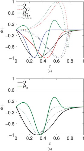
Figure 4 compares the spatial reaction rate variation of main species and heat release rate for the three flames. The superscript + indicates quantities normalized using their maximum values. The species’ net reaction rates and heat release rate are plotted together to highlight salient features of the multi-component fuel-air flame. Here, the progress variable is based on temperature (for reasons that will become apparent later). The maximum heat release rate occurs around c = 0.68 in the methane flame and around c = 0.3 for the multi-component fuel flame. A similar behaviour is observed for the hydrogen flame shown in Figure 4b. The heat release zone thickness, , defined as the spatial thickness over which the heat release drops to 5% of its maximum value, is mm for the multi-component fuel flame, 5.3 mm for the methane flame, and 4.9 mm for the hydrogen flame. Thus, the multi-component fuel flame has the widest heat release zone. The net reaction rates of CO, H₂, and CH₄ are found to coincide with the heat release zone and to have approximately the same width for the methane flame. These zones are distinct for the multi-component fuel flame; CH₄ consumption peaks just before the peak heat release, H₂ consumption peaks just after it, and CO consumption peaks later than peak heat release. The consumption of H₂ is across all c in the hydrogen flame as one would expect, but it is produced around c =0.1 and 0.6 in the multi-component fuel flame as in Figure 4b. It is also worth noting that CO consumption by magnitude is larger than the rest of the fuel species because of the abundance of CO in the multi-component fuel.

Figure 4 Comparison of main fuel species reaction rates and heat release rate in (a) multi-component fuel-air and CH₄-air and (b) multi-component fuel-air and H₂-air flames. The values are normalized using the respective maximum magnitudes.

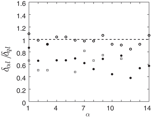
Another point to note is that the reaction zone widths are different for different fuel species present in the multi-component fuel. To shed more light on this, the laminar reaction zone thickness for species α, , defined as the thickness over which the reaction rate falls to 5% of its maximum value, is calculated and compared to . The results are shown as in Figure 5 for the first 14 species listed in Table 1. One observes that all major species in the methane flame have in contrast with the other two flames. The reaction zone thickness for the majority of species in the hydrogen flame is smaller than . For the multi-component fuel flame, CH₄ (α = 12, see Table 1) has the thinnest reaction zone, which is less than half of the heat release thickness. H₂O has the thickest reaction zone in both the methane and multi-component fuel flames. In comparison, the laminar flame thickness based on the temperature gradient, δ_ι, is smaller than the minimum species reaction zone thickness. This implies that resolution requirements based on δ_ι or δ can be more stringent. Due care must thus be exercised to numerically resolve the minimum reaction zone thickness in skeletal chemistry DNS.

Figure 5 Species reaction zone thickness normalized by the heat release zone thickness. Index α as in Table 1. Filled circles: multi-component flame; open circles: methane flame; squares: hydrogen flame.

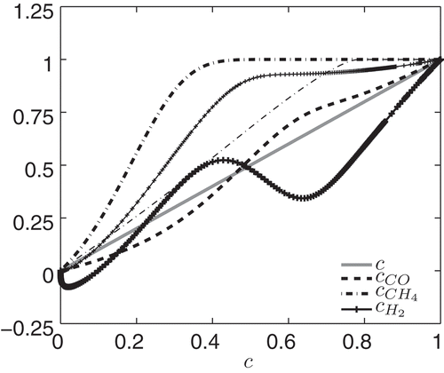
Figure 6 shows the variation of different progress variables based on fuel species with c. In particular, , and are shown for the three laminar flames considered. Thick lines are for the multi-component fuel flame, thin dashed-dotted line is for in the methane flame, and the symboled (+) thin line is for in the hydrogen flame. Consistent with the results shown in Figures 4 and 5, CH₄ is consumed at relatively low temperatures yielding an increase in for both the multi-component and methane flames. However, all of the methane is consumed in the multi-component flame by about c = 0.4, in contrast to the methane flame showing CH₄ consumption up to c = 0.8. The behavior of is very different: a monotonic variation in the hydrogen flame and a non-monotonic variation in the multi-component flame.

Figure 6 Different progress variables definitions against c based on temperature. Thick lines: multi-component flame; thin dashed-dotted line: methane flame, ; thin line with + hydrogen flame, .

A careful examination of H₂-related reactions reveals the reactions 2, 3, 12, 44, 47, and 48 given in table 3 of Nikolaou et al. (2013), to be the dominant ones. Out of these six reactions, H₂ is consumed by only reaction 2 across c space. Reactions 44, 47, and 48 produce H₂ through a consumption of CH₄ at low c. This explains H₂ production around c = 0.1 observed in Figure 4. Reaction 3 has a dual role: at lower c it consumes H₂ and at larger c it produces H₂ (Das et al., 2011). This would explain the production of H₂ around c = 0.6 observed in Figure 4 leading to low seen in Figure 6. The difference in noted above also warrants an explanation. CH₄ consumption occurs through reactions 41, 42, and 47, and reaction 42 has the lowest activation energy and highest consumption rate at low c. The presence of water vapor in the fuel mixture yields a large amount of OH leading to an increased consumption of CH₄ through reaction 42 (Das et al., 2011; Singh et al., 2012). In the methane flame, OH radicals come only through elementary reactions involving methane and oxygen, e.g., reaction 41, and these reactions usually have high activation energy.

Post-Processing Method

The global flame behavior is analyzed through the calculation of the consumption speed defined as:

(6)

where is the total area in the homogeneous direction and the integral is taken over the entire computational volume V. Figure 7 shows the temporal evolution of for the two cases and the time is normalized by the flame time , which is common for both cases. One flame time corresponds to about 20.2 large eddy turn-over times for case B and 3.5 large eddy turn-over times for case A.

Figure 7 Consumption speeds for the two turbulence levels.

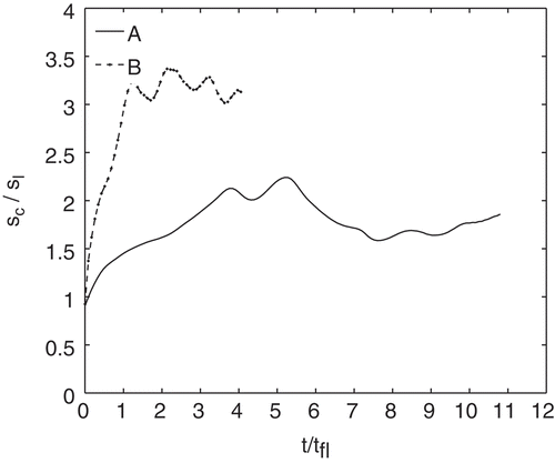
Initially, is approximately equal to for both cases, and case B reaches a quasi-stationary state after about one and remains there for the duration of this simulation . Case A shows a slower evolution: increases up to about and remains in a more or less quasi-stationary state up to about . The consumption speed drops for because the flame is observed to slowly move out of the computational domain.

The DNS data are post-processed with the same spatial differencing schemes used in the DNS. Averaging is done both in space (in the homogeneous y and z directions) and time, and by combining adjacent spatial points in order to increase the statistical accuracy. Five neighboring planes are combined, after ensuring that the statistics, such as the x-wise averages, and the pdfs of c are not affected unduly. The average value of a quantity V at point i in x direction is calculated using

(7)

where N_p = 5. The index (i − 3) indicates that the averaging is symmetric about point i for points well away from the boundaries. Due care is taken at the boundaries. For case A, time averaging is performed between 3.52 and 5.6t_fl, and for case B time averaging is performed between 1.0 and 3t_fl as per the results in Figure 7. During these two intervals, the flames seem to be in a quasi-stationary state at least as far as s_c is concerned. Conditional averages, to be discussed later, are taken over the entire volume in bins of c, and time-averaged over the above time intervals.

The flame surface is identified as c = c* iso-surface with c* = 0.32 corresponding to the peak heat release in an unstrained laminar flame. The use of temperature-based c is justified by the fact that mass fraction-based progress variables vary substantially depending on the species as one may see in Figure 6. The flame normal vector components are given by:

(8)

where . The generalized flame surface density (FSD) is with the over-bar denoting an LES filtering operation (Boger et al. 1998). In the limit of zero filter width and using a Gaussian filter, , where σ is the surface density function (SDF).

The flame stretch Φ is given by (Candel and Poinsot, 1990):

(9)

where a_t is the tangential strain rate and K_m is the surface mean curvature. The displacement speed defined as can be obtained using the transport equation for T, since c is defined using temperature. Thus, after neglecting compressibility effects, which are expected to be small for the flames of this study, s_d at every point on the flame surface is calculated using (Poinsot and Veynante, 2005):

(10)

where is the heat release rate. The flame surface related quantities are normalized as follows: , and density weighted displacement speed is .

Probability density functions of s_d, K_m, a_t, and Φ are extracted by identifying iso-surfaces of c = 0.1, 0.32, 0.5, and 0.7. These pdfs are obtained using the samples collected over the entire sampling period on these specific iso-surfaces and surface averages are calculated by taking the moment of these pdfs. Before presenting these results, the flame structure is discussed in the next section.

Turbulent Flame Structure

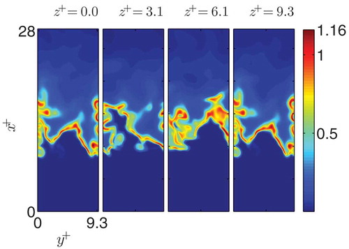
The instantaneous spatial variations of normalized heat release rate, , in cases A and B are shown in Figures 8 to 10. The local heat release rate is normalized as , where is the maximum heat release rate in the multi-component fuel laminar flame used in the previous section. The typical contours of are shown in x-y planes taken at various z locations and the spatial distances are normalized using δ_l. The result is shown for case A at t = 4t_fl and two instances, t_fl and 2t_fl, are shown for case B. The flame structure in case A resembles that of a laminar flame wrinkled by large-scale turbulence. This structure in case B is different and heat release contours are patchy as in Figure 9. The local break up in heat release rate primarily results from flame–flame interactions allowing pockets of reactants to exist in the product zone. This leads to the formation of local hot spots behind the “main” reaction zone, as one observes in Figures 9 and 10. Also, there are regions of high positive curvature (convex to the reactant side) trying to advance into the reactants (3rd frame in Figure 9 and 2nd frame in Figure 10), which eventually break apart due to excessive heat losses. It is found that heat release is maximized in negatively curved regions for both cases, consistent with previous studies of methane-air (Echekki and Chen, 1996) and hydrogen-air (Tanahashi et al., 1999) combustion.

Figure 8 Contours of for case A at .

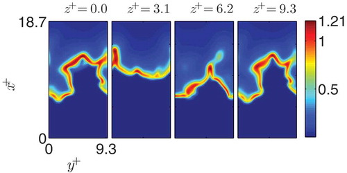
Figure 9 Contours of for case B at .

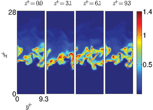
Figure 10 Contours of for case B at .

A stoichiometric hydrogen-air flame with , and T_r = 700 K was simulated by Tanahashi et al. (1999), using a detailed mechanism and these conditions are similar to the inlet conditions for case A. It was observed (Tanahashi et al., 1999) that high heat release rate regions were unconnected and isolated in space, which are consistent to the observation made here for case A. Similar results were reported also for a lean (φ = 0.8) methane-air flame in the study of Bell et al. (2002) (see their Figure 1) and this flame had and and included a detailed chemical mechanism. This flame structure resembles that of corrugated flamelets regime having and in the classical combustion regime diagram (Peters, 1988). Figure 3 shows that the filled circle is the best possible case in this study for this regime, and this condition is based on the inlet turbulence parameters. Case B, on the other hand, has a flame structure resembling that of distributed reaction zones because it is more difficult to identify a clear continuous flame front for most parts of the simulation period. The distributed reaction zones regime (Peters, 1988) has Ka > 1 and Da < 1, and the filled black square in Figure 3, based on the inlet turbulence parameters, is the closest possible choice in this study. It is worth noting the Da and Ka values given in Table 3 in this regard suggest that the various limits for combustion regimes in Figure 3 are debatable.

c-Space Comparison with Laminar Flame Profiles

The scatter plots of heat release rate and some of the species mass fractions are shown in Figure 11 for case B (similar results with less scatter are observed for case A and thus they are not shown here). The superscript + indicates that the quantities are normalized using the respective maximum in the multi-component fuel-air laminar flame discussed earlier. The continuous gray lines show the conditional average and the dashed gray lines show the unstrained laminar flame results.

Figure 11 Variation of normalized species mass fractions and heat release rate with c for case B at . Continuous gray line shows the conditional average, and dashed line shows the laminar flame result.

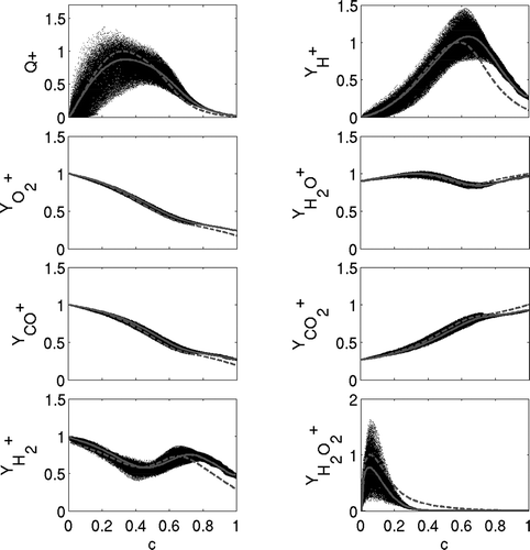
There is a large scatter in the heat release rate for 0.0 < c < 0.6, and specifically around c = 0.2. This is expected because turbulence in this region is stronger. As a result, the heat release fluctuates significantly above and below the laminar value with local drop occurring relatively frequently. The heat release rate drops to zero for c = 0. 1 and below implying local extinction in some regions near the leading edge of the flame.

The variation of normalized mass fractions of O₂, H₂O, CO, CO₂, and H₂ show minimal scatter for both cases considered and a very good agreement with the laminar flame result is seen. A similar agreement was observed for CH₄ and OH. Relatively larger deviations from the laminar flame are observed for H, H₂, and H₂O₂. Similar results were observed to be true for HCO and O. For all of these cases, however, the conditional average was found to be in good agreement with the laminar flame result.

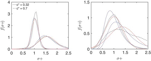
These results imply that an unstrained flamelet model would be a reasonable model to represent the flame structure of the flame studied here. To shed more light on this, pdfs of SDF, σ, for c* = 0.1, 0.32, 0.5, and 0.7 shown in Figure 12 are studied. The mean, μ, and standard deviation of σ are given in Table 5 (other quantities given in this table will be discussed later). The SDF on each iso-surface is normalized according to using the SDF value of the laminar flame on the same iso-surface, . Thus, σ⁺ is a measure of thinning or thickening of the flame front. The thinning is indicated by σ⁺ > 1 and thickening is indicated by σ⁺ < 1. For both cases A and B, the mean values in Table 5 are smaller than 1 for c^* = 0.1 indicating that the leading sides are thickened on average by turbulence. The strongly heat releasing regions around the c* = 0. 32 iso-surface do not thicken or thin and it also has the lowest standard deviation suggesting that the influence of turbulence is minimal. As one moves towards the product side, the mean value of σ⁺ increases above 1 implying flame thinning. Thus, turbulence acts to bring iso-surfaces together in the product side and it acts to move iso-surfaces apart in the reactant side. This means that the flame front broadens for low c* and thins for high c*, which is similar to the observation by Sankaran et al. (2006) for a lean methane-air premixed slot-jet flame near the jet exit . The current results are also consistent with previous premixed flame DNS studies involving 1-step chemistry (Hamlington et al., 2010; Kim and Pitsch, 2007) at high turbulence level.

Table 5 Mean μ and standard deviation std for surface variables for cases A and B

c*	μ	std	μ	std	μ	std	μ	std	μ	std	μ	std
Case A
0.1	1.123	0.555	0.974	0.488	−0.090	2.484	0.743	0.771	0.033	3.571	0.962	0.168
0.32	1.421	0.672	0.947	0.448	−0.026	1.981	0.789	0.732	0.007	3.579	1.033	0.155
0.5	1.667	0.859	0.956	0.526	0.040	1.768	0.727	0.665	−0.019	3.668	1.207	0.200
0.7	2.063	1.098	1.028	0.569	0.160	1.865	0.489	0.496	−0.116	4.310	1.570	0.372
Case B
0.1	1.282	1.182	1.06	1.128	−0.341	4.636	2.390	3.721	−0.087	6.956	0.885	0.387
0.32	1.657	1.389	1.127	1.038	−0.431	3.960	2.241	3.184	−0.042	6.687	1.014	0.385
0.5	1.912	1.628	1.135	1.086	−0.174	3.604	1.889	2.831	0.116	6.861	1.187	0.459
0.7	2.118	1.956	1.234	1.196	0.487	3.423	1.347	2.302	1.055	7.065	1.364	0.559

Figure 12 Pdfs of normalized SDF, σ⁺, for case A (left) and case B (right).

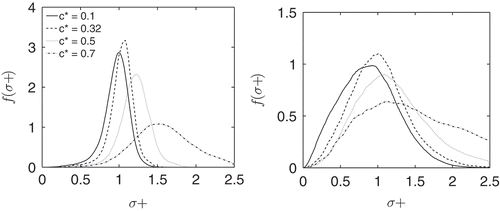
The flamelet nature of turbulent combustion can also be inferred using the σ⁺ pdfs in Figure 12. If this pdf has a narrow peak around σ⁺ = 1 then the combustion is flamelet-like. The spread of this pdf, denoted by the standard deviation of σ;⁺, suggests the influence of turbulence. A standard deviation of zero indicates a laminar flame and thus for an unsteady laminar flamelet. The turbulence will smear this delta function and so the shape of depends on turbulence parameters and c* value. With these considerations, one may say that the turbulent flame is strictly flamelet-like if or that . For extremely high turbulence, one would expect that . This is so because c gradients will be low as increases and the probability for σ⁺ = 0 becomes increasingly larger. Hence, in the PSR limit it is expected that . Although, this PSR limit is not seen here, the probability for σ⁺ < 1 for all c* in case B is larger compared to case A. The mean and standard deviation values in Table 5 suggest that the combustion in case A is more flamelet-like than in case B supporting the above deduction using the resulting pdfs in Figure 12.

The SDF, σ, is closely related to the scalar dissipation rate, N, through , where is the thermal diffusivity of the mixture and N=. Previous studies of premixed (Swaminathan and Bilger, 2001) and non-premixed (Hawkes et al., 2007) combustion showed that f (N⁺), the scalar dissipation rate pdf, is approximately log-normal. To test whether this applies for the σ⁺ pdfs, and for the multi-component fuel mixture considered here, Figure 13 shows for c* = 0.32 (where heat release peaks in the laminar flame) and 0.7 the σ⁺ pdfs as extracted from the DNS against the pdf models using both the log-normal and normal distributions. The model pdfs are taken to have the same mean and variance as the σ⁺ pdfs. Figure 13 shows that the log-normal pdf gives a good agreement with the DNS data for both turbulence levels, in agreement with previous studies. For both cases, however, the log-normal pdf shows some negative skewness in comparison with the actual pdfs. The normal pdf, on the other hand, seems to give an improved agreement, especially for case B. Further DNS at intermediate and higher turbulence levels will help to correctly parameterize the σ⁺ pdfs and establish limits on the flamelet regime.

Figure 13 Pdf model comparison for σ, for and 0.7. Blue lines: log-normal pdf and red lines: normal pdf. Both pdf models have the same mean and variance as the σ pdfs obtained from the DNS.

Surface Pdfs and Scatter Plots

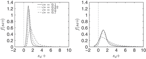
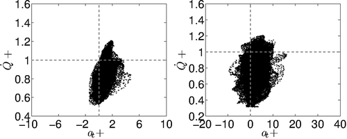
Figure 14 shows displacement speed pdfs, , for cases A (left) and B (right) for four c* iso-surfaces. The pdfs peak for and shift to higher values as c* increases since the flow accelerates across the flame due to dilatation. The mean and standard deviation of are given in Table 5 and these values increase with c* in agreement with previous studies (Chakraborty, 2007). An important difference between cases A and B is the finite probability for negative displacement speed in case B. We shall revert to this negative displacement speed later in this subsection.

Figure 14 Displacement speed pdfs for cases A (left) and B (right).

The pdfs of surface mean curvature, K_m, shown in Figure 15 for cases A and B, are Gaussian-like, consistent with previous DNS studies both in 2D with skeletal chemistry and in 3D with 1-step chemistry (Chakraborty, 2007; Echekki and Chen, 1996). The curvature pdfs in case A peak around 0 and have, in general, smaller standard deviations than for case B, which can also be seen in Table 5. This implies that the probability of having high positive curvatures is larger in case B than in case A and it supports having nonzero probability for negative displacement speed as one shall see later. The curvature pdfs have negative mean values for c* = 0. 1 and 0.32 in case A and for c* = 0.1 and 0.32 and 0.5 in case B (see Table 5). At the same time, the mean values implied by the pdfs of , shown in Figure 16, is positive for all c* suggesting that the curvature sign affects the stretch rate primarily. The variation of mean given with c* in Table 5 is consistent with previous studies (Chakraborty, 2007; Echekki and Chen, 1996). These results indicate that the probability of having is larger than for .

Figure 15 Curvature pdfs for cases A (left) and B (right). Lines are as in Figure 14.

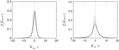
Figure 16 Tangential strain pdfs for cases A (left) and B (right).

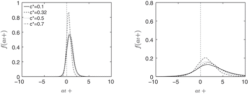
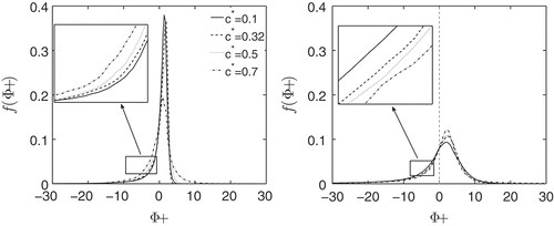
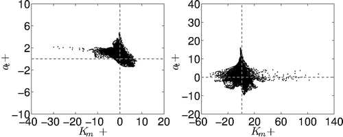
A comparison of the stretch rate pdfs in Figure 17 shows that there is a lower probability for Φ⁺ < 0 at low c* in case A. This gives positive mean stretch rates for low c*, and negative mean stretch rates for higher c*. Since , iso-surface area is produced on the leading side and is destroyed for higher c* values in case A. An opposite trend is observed for case B: the mean stretch rate is negative for low c* and positive for high c* values. This is reflected in the stretch rate pdfs shown in Figure 17. This can be attributed to stronger turbulence in regions of c < 0.1 in case B causing (1) local extinction of the leading flame elements as one may see from Figures 10 and 11, and (2) significant flame–flame interaction, which also destroys flame surface area. These processes result in negative mean stretch rates. Flame elements at higher c*, however, interact with less intense turbulence and are thus less likely to extinguish or experience flame–flame interaction, resulting in positive mean stretch rates (see Table 5).

Figure 17 Stretch rate pdfs for cases A (left) and B (right).

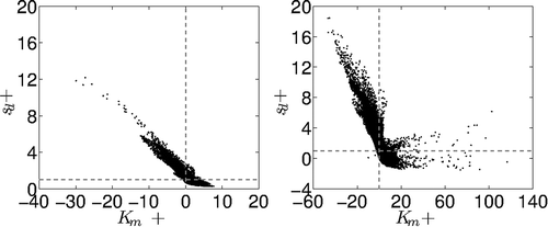
Figure 18 shows a scatter plot of against on the c* = 0.32 iso-surface. No correlation with tangential strain rate was observed. The negative displacement speed is seen only for as observed in earlier studies (Chakraborty, 2007; Chakraborty and Cant, 2004; Gran et al., 1996). It was shown in these studies that the displacement speed can be decomposed into four components: , where s_r, s_n, s_t, and s_v, respectively, denote contributions from reaction, normal diffusion, tangential diffusion, and species diffusion. The contribution of s_v is found to be negligible for the cases of this study. It was shown in an earlier 2D simulation of methane-air combustion that the contribution of s_t is small, on average, and that the pdf of s_d can be recovered quite well by considering the contributions of s_n and s_r only (Peters et al., 1998). This was also confirmed in a later 3D simulation with 1-step chemistry (Chakraborty and Cant, 2004). Both of these studies also noted, however, that a finite probability for was not recovered reasonably. However, including s_t while modeling flame stretch (Peters, 1999) was shown to be responsible for (Hawkes and Chen, 2005). This is because s_t is proportional to the curvature since (Chakraborty 2007; Chakraborty and Cant, 2004; Gran et al., 1996). Negative displacement speeds thus occur in regions of high positive curvature where s_t contribution exceeds s_r and s_n contributions (Chakraborty, 2007, Chakraborty and Cant, 2004).

Figure 18 Displacement speed against curvature for cases A (left) at , and B (right) at , for .

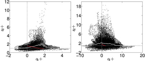
Figure 19 also shows conditional averages, . The displacement speed does not show any significant correlation with but the correlation with is strong as shown in Figure 18. The response in strained flames of multi-component fuel-air mixture in reactant-to-product (RTP) configuration for the same thermo-chemical conditions as for the DNS is shown in Figure 19 as a red line. The RTP flames are computed using the OPPDIF code and s_d on the iso-surface is extracted and shown in Figure 19. The strain rates for the RTP flame are increased up until the flame first coincides with the stagnation point location. A good correlation between extracted from DNS and strained flames of a lean methane-air mixture was observed by Hawkes and Chen (2006) and the current results are contrary to this earlier observation. For the current laminar flames s_d decreases with increasing strain rate suggesting a thermo-diffusively stable flame but the conditional average from the turbulent flames is much different. For case A, the conditional average shows that s_d increases slightly for relatively small positive strain rates and it decreases for positive strain rates in case B. In either case, the agreement with the strained laminar flame response is poor due to the strong role of turbulence in the multi-component fuel combustion and the presence of various fuel species of widely differing thermo-diffusive characteristics. The conditional average suggests that the DNS flame seems to be thermo-diffusively stable for large and unstable for small when the turbulence level is small (as in case A). The flame is stable for in case B having substantially larger compared to case A. Since curvature is the main variable affecting s_d, the displacement speed is negative in regions with large positive curvatures in case B as theory suggests (Chakraborty, 2007; Chakraborty and Cant, 2004). Since the turbulence level is relatively small in case A, is not observed for this case. This observation is also supported by the curvature pdfs shown in Figure 15 for the two cases.

Figure 19 Displacement speed against tangental strain for cases A (left) at , and B (right) at , for . Gray line: conditional average. Red line: strained RTP flame computation.

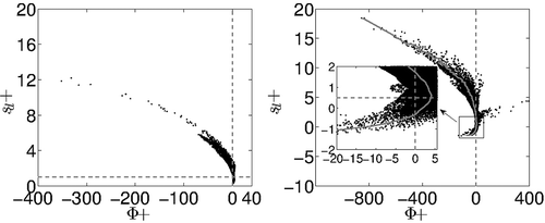
Another important point in Figure 18 is that s_d can be as much as 10 times larger than s_l when . To shed more light on this, the variations of normalized heat release rate with and are shown as scatter plots in Figures 20 and 21, respectively. Results for both cases A and B are shown. The heat release rate is maximum in regions of negative and with the value being around 20% larger than maximum laminar flame value. Although there is some correlation of with , the correlation with is much stronger. Furthermore, the increase in in regions with large negative is too modest to explain the increase in values observed at these locations. The positive contribution of s_t in regions with negative is important as noted in previous studies (Chakraborty and Cant, 2004). A similar correlation to that observed in this study was also observed in an earlier 2D simulation of hydrogen-air combustion with (Baum et al., 1992, 1994). For these mixtures maximum heat release rate decreased with increasing curvature as seen in Figure 20, while for leaner mixtures , which are thermo-diffusively unstable, the opposite trend was observed. Similar observations were made by Chen and Im (2000) by studying consumption speed (directly related to heat release rate), curvature, and strain rate correlations in 2D hydrogen DNS for a stable mixture . Also, a significant correlation was also observed by Chen and Im (2000), which is contrary to the findings of this study. Later, 3D methane DNS (, Bell et al., 2002) also revealed a strong correlation, which was also seen further in 2D DNS of premixed methane and propane flames (Bell et al., 2007).

Figure 20 Heat release against curvature for cases A (left) at , and B (right) at , for .

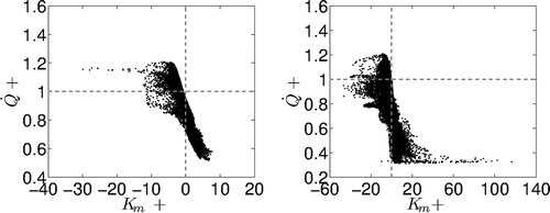
Figure 21 Heat release rate against tangential strain rate for cases A (left) at , and B (right) at , for .

In order to check the correlation, Figure 22 shows a scatter plot of versus . This correlation is weakly negative for case A with negative strain appearing for positive curvature similar to that observed for a lean methane flame by Chakraborty et al. (2008). There is no clear correlation for case B as seen in Figure 22, although the peak strain rate occurs near-zero to small negative curvature values. This is also similar with the strain rate-curvature relation observed for the lean hydrogen mixture considered by Chakraborty et al. (2008). This difference is due to a higher turbulence level in case B resulting in higher dilatation rates in regions with negative curvature. As a result the normal component of the dilatation (and strain rate) increases, thus lowering the correlation of the tangential straining with curvature.

Figure 22 Tangential strain rate against curvature for case A (left) at , and case B (right) at , for .

Figure 23 shows the variation of against on the iso-surface. The conditional average is also shown for case B to elucidate and understand the variation with . For small curvature and strain rates, i.e., for small stretch values, theory suggests that the variation of s_d with is linear and it is given by (Buckmaster and Ludford, 1982; Williams, 1985):

Figure 23 Displacement speed against stretch rate for case A (left) at , and case B (right) at , for . Gray continuous line shows the conditional average for case B.

(11)

where Ma is the fuel Markstein number, which is essentially . The results in Figure 23 suggest that the variation of displacement speed with stretch rate is nonlinear and there are significantly large negative stretch rates with low probability. Most of the flame experiences low stretch rates. These results are consistent with earlier observations for methane-air combustion in 2D turbulence (Chen and Im, 1998). When the stretch rate is small and positive, and , the above linear relation is reasonable as theory suggests. The positive Ma suggests a thermo-diffusively stable flame. When the stretch rate is large and negative and s_d is positive, Ma is observed to decrease because for large positive s_d (Chen and Im, 1998). Since large positive displacement speeds occur in regions with large negative curvature (and large negative stretch rate), Ma is positive and decreases in accordance with the nonlinear variation observed in Figure 23.

From the inset in Figure 23 for case B, it is observed that Ma changes sign at . Furthermore, the linear relation between and for positive stretch rates holds for . It was concluded by Mishra et al. (1994) that the linear relationship holds for normalized stretch rates less than 0.1 by analyzing outwardly and inwardly propagating laminar spherical flames computed with 1-step chemistry. The stretch rate was normalized by Mishra et al. (1994) using and the value of 5 obtained in the present work translates to 0.32 when is used for normalization. Furthermore, it was found (Mishra et al., 1994) that the linear region can be extended up to a normalized stretch rate of 0.5 with an error less than 5%. Thus, the linear region is extended up to , which is in agreement with the results of this study. For negative stretch rates, the linearity begins to deteriorate because Ma is observed to gradually change. Despite this, the relationship between and is observed to be approximately linear for and as one can see in the inset of Figure 23 for case B. Thus, the strongest nonlinear variation of with is observed for medium negative stretch rates, which was also observed by Mishra et al. (1994) for flames with Le > 1. These results suggest that the use of a linear relation in Eq. (11) to study premixed flames in large turbulence is limited and caution must be exercised.

Modeling

In this section, the performance of some common mean reaction rate closures are evaluated for the multi-component fuel flame in the RANS context. Although LES is becoming more popular, RANS often forms the basis for LES model development and is still used in industry but also in hybrid RANS/LES codes. In addition, since this is the first DNS study of multi-component fuel combustion, it is prudent to initially conduct the analysis in the RANS context. The chemical complexity of the fuel coupled with the relatively large turbulence levels considered here present the most stringent test for all mean reaction rate models since the vast majority of these models were validated using 1-step chemistry DNS data in 3D, or skeletal chemistry DNS data in 2D. A brief description of the models evaluated here is given below.

1. Eddy break up model (EBU) of Spalding (1971, 1977):

   (12)

   where C_ebu is the model constant of order unity. In this study, C_ebu = 3.26 for case A and 2.43 for case C. These values are found to give improved agreement with the DNS data.

2. Algebraic closure of Bray and Moss (1977):

   (13)
   (14)

   where , ζ is the sample space variable for the progress variable, and f (ζ) is the burning mode pdf obtained using the progress variable gradient in the laminar unstrained flame. For this flame C_m is found to be equal to 0.55. In Eq. (13), the following closure is used by Kolla et al. (2009):

   (15)

   and in Eq. (14) the scalar dissipation rate extracted from the DNS is used instead. This model was observed to give reasonable results with the DNS data, and details can be found in Kolla et al. (2009). This comparison will help elucidate the effect of the scalar dissipation rate model on the actual performance of the Bray closure. These models will henceforth be referred to as Bray-1 (Eq. (13)) and Bray-2 (Eq. (14)).

3. Unstrained flamelet model (Bradley 1992):

   (16)

   where ζ is the sample space variable for the progress variable c, and f (ζ) is a presumed progress variable pdf:

   where is taken to be a β-function:

   and , , .

4. Generalized flame surface density (FSD) model (Boger et al., 1998; Bray et al., 1989; Candel et al., 1988; Marble and Broad-well, 1977; Pope, 1988). Neglecting the contribution of diffusive effects, the mean reaction rate can be closed as:

   (17)

   where (here in the RANS context), and the bar in Eq. (17) denotes the average on a c* iso-surface. A common assumption is . Table 5 shows that is approximately equal to unity across all c* considered, justifying the use of this assumption for this fuel.

5. Strained flamelet model by Kolla and Swaminathan (2010):

   (18)

   In the strained flamelet model the flame is assumed to be an ensemble of strained laminar flamelets. The flamelets are evaluated in the RTP (reactant to product) configuration for increasing strain rate values. A table is then built for , where ζ is the sample space variable for c, and is the sample space variable for the strain rate. The conditional pdf is assumed to be log-normal:

   and its shape at each point in the domain depends on the mean conditional scalar dissipation rate . μ is calculated using the relationship: , and σ is taken to be 0.3 from Kolla and Swaminathan (2010). Further details of this model can be found in Kolla and Swaminathan (2010).

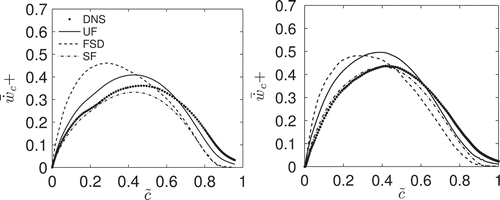
Figures 24 and 25 show the mean progress variable reaction rate estimated using the above five models against the DNS data for cases A and B, respectively. The EBU model shows the best overall agreement across the flame brush; however, one has to adjust the model constant C_ebu. The value of this constant inevitably depends on the combustion configuration, mixture composition, and the turbulence characteristics. The algebraic closure of Bray (Eq. (13)) gives a good agreement for but slightly overestimates the mean reaction rate for . If the same model but using Eq. (14) is used instead, the agreement becomes somewhat better for , but for the mean reaction rate is slightly underestimated. The discrepancies observed for this model are primarily owing to the finite flame thickness and the departure of the progress variable pdf from the bimodal shape, which the model assumes. These effects become more important as the turbulence level increases which explains the large overprediction of the Bray model observed in Figure 24 for case B. The unstrained flamelet model shows a good agreement with the DNS data for both turbulence levels with some overprediction in the range . It was observed that this is a result of the corresponding overprediction of the burning mode pdfs in the same region, implying that an improved pdf model can render even better agreement for the unstrained flamelet model. The FSD model shows a reasonable agreement: it slightly overestimates the mean reaction rate in the range for case A, while for the mean reaction rate is underestimated. This may be a result of the lack of straining effects in this model formulation. The strained flamelet model shows an excellent agreement for relatively low values, while at high values it underestimates and collapses with the FSD model. For relatively low values, turbulence-scalar interaction is stronger and diffusive effects that are not accounted for in the FSD model become important. This may explain the slight overestimation when using Eq. (17). Although all the models tested here seem to give reasonable agreement, some tuning of model parameters seems to be inevitable. Further analyses are required if model tuning is to be avoided and this is beyond the scope of this study.

Figure 24 EBU model, and Bray’s model using (Bray-1) and (Bray-2). Case A (left) and case B (right). Case A: . Case B: .

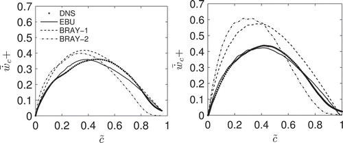
Figure 25 Unstrained flamelet model (UF), FSD model and strained flamelet model (SF). Case A (left) and case B (right).

CONCLUSIONS

Direct numerical simulation of turbulent premixed combustion of a multi-component fuel with air in three physical dimensions has been performed. The fuel consists of CO, H₂, H₂O, CH₄, and CO₂ in proportions akin to BFG or a low calorific value syngas mixture. The simulations employed a skeletal mechanism with 49 reactions and 15 species, developed specifically for such complex fuels (Nikolaou et al., 2013). The simulations are performed for two flames having a Damkohler number of 5.19 and 1.17 based on the inflowing turbulence parameters.

The multi-component fuel flame shows a substantially more complex structure than most traditional single-component fuel flames. Heat release occurs over a wider temperature range, which produces a thicker flame front. There are distinct and non-overlapping species consumption and heat releasing zones. The peak CH₄ consumption in the multicomponent fuel flame occurs at low c values, which is followed by peak H₂, O₂, and CO consumptions.

Despite a large scatter in heat release rate and in species mass fractions, their conditional averages are observed to be in good agreement with the unstrained laminar flame results. Probability density functions of displacement speed, curvature, strain, and stretch rate, across the flame brush, are observed to be in good agreement with previous findings using 1-step chemistry DNS data. The stretch rate pdf does show some variation with c*, and thus if one can use flame-surface-based approaches to model these flames is an open question. Thickening of the preheat region and thinning of the reactive-diffusive region observed in this study, are also consistent with 1-step DNS. An important difference for the multi-component fuel flame, is that the standard deviation of the normalized generalized FSD increases towards the product side. This is suggestive of a wider distribution of the heat release rate, giving rise to large probabilities for the generalized FSD at relatively high c* values. A Gaussian pdf of the normalized FSD is found to be a better model candidate than a log–normal pdf, which is in contrast to earlier findings. Five different mean reaction rate closures are evaluated for the multi–component fuel flame in the RANS context. These are the EBU model, the algebraic closure of Bray, the unstrained flamelet model, an FSD model, and a strained flamelet model. Overall, the EBU model shows a very good agreement provided that the model constant is adjusted appropriately. The unstrained flamelet model is also found to give a good agreement with the DNS data.

Heat release and displacement speed are shown to correlate strongly with curvature and not with strain rate. Their peak values are observed in locations with negative curvatures (convex towards the products side). The same behavior is observed for the radicals H, OH, and O, which peak well behind the heat release zone. CO₂ on the other hand was found to peak in positive curvature regions instead, due to its large concentrations in the reactant mixture.

Overall, the complexity of the fuel mixture has a significant effect on the flamelet structure of the unstrained laminar flame, and the fluid dynamic strain does not change this structure unduly. The chemistry–turbulence interaction did impart some subtle changes but these changes do not seem to be statistically significant. This could be because of the very low amount of hydrogen present in the mixture and the near unity Lewis number of the rest of the species present. Thus, the classical flamelet modeling approach can be employed for turbulent flame calculations.

ACKNOWLEDGMENT

ZMN and NS acknowledge Prof. S. Cant for the DNS code.

FUNDING

ZMN and NS acknowledge the funding through the Low Carbon Energy University Alliance Programme supported by Tsinghua University, China. ZMN acknowledges the educational grant through the A.G. Leventis Foundation. This work made use of the facilities of HECToR, the UK’s national high-performance computing service, which is provided by UoE HPCx Ltd at the University of Edinburgh, Cray Inc and NAG Ltd, and funded by the Office of Science and Technology through EPSRC’s High End Computing Programme.

Additional information

Funding

ZMN and NS acknowledges the funding through the Low Carbon Energy University Alliance Programme supported by Tsinghua University, China. ZMN and NS also acknowledge Prof. S. Cant for the DNS code. ZMN acknowledges the educational grant through the A.G. Leventis Foundation. This work made use of the facilities of HECToR, the UK’s national high-performance computing service, which is provided by UoE HPCx Ltd at the University of Edinburgh, Cray Inc and NAG Ltd, and funded by the Office of Science and Technology through EPSRC’s High End Computing Programme.

References

- Baum, M., Poinsot, T.J., and Haworth D.C. 1992. Numerical simulation of turbulent premixed H2/O2/N2 flames with complex chemistry. In Proceedings of the Summer Program, Stanford University & NASA-AMES, pp. 345–346.
- Baum, M., Poinsot, T.J., Haworth, D.C., and Darabiha N. 1994a. Direct numerical simulation of H2/O2/N2 flames with complex chemistry in two-dimensional turbulent flows. J. Fluid Mech., 281, 1–32.
- Baum, M., Poinsot, T., and Thevenin, D. 1994b. Accurate boundary conditions for multicomponent reactive flows. J. Comput. Phys., 116, 247–261.
- Bell, J.B., Cheng, R.K., Day, M.S., and Sheperd, I.G. 2007. Numerical simulation of Lewis number effects on lean premixed turbulent flames. Proc. Combust. Inst., 31, 1309–1317.
- Bell, J.B., Day, M.S., and Grcar, J.F. 2002. Numerical simulation of premixed turbulent methane combustion. Proc. Combust. Inst., 29, 1987–1993.
- Boger, M., Veynante, D., Boughanem, H., and Trouvé, A. 1998. Direct numerical simulation analysis of flame surfacce density concept for large eddy simulation of turbulent premixed combustion. Proc. Combust. Inst., 27, 917–925.
- Bradley, D. 1992. How fast can we burn? Proc. Combust. Inst., 24, 247–262.
- Bray, K.N.C., Champion, M., and Libby, P.A. 1989. The interaction between turbulence and chemistry in premixed turbulent flames. In R. Borghi and S.N.B. Murthy (Eds.), Turbulent Reactive Flows, Lecture Notes in Engineering, Springer Verlag, pp. 541–563.
- Bray, K.N.C., and Moss, J.B. 1977. A unified statistical model of the premixed turbulent flame. Acta Astronaut., 4, 291–319.
- Buckmaster, J., and Ludford, G. 1982. Theory of Laminar Flames, Cambridge University Press, Cambridge, UK.
- Candel, S.M., Maistret, E., Darabiha, N., Poinsot, T., Veynante, D., and Lacas, F. 1988. Experimental and numerical studies of turbulent ducted flames. Proceedings of the Marble Symposium, Caltech, Pasadena, CA, August.
- Candel, S.M., and Poinsot, T. 1990. Flame stretch and the balance equation for the flame area. Combust. Sci. Technol., 70, 1–15.
- Cant, R.S. 2012. SENGA2 user guide. Cambridge University technical report: CUED/ATHERMO/TR67.
- Chakraborty, N. 2007. Comparison of displacement speed statistics of turbulent premixed flames in the regimes representing combustion in corrugated flamelets and thin reaction zones. Phys. Fluids, 19, 105–109.
- Chakraborty, N., and Cant, R.S. 2004. Unsteady effects of strain rate and curvature on turbulent premixed flames in an inflowoutflow configuration. Combust. Flame, 137, 129–147.
- Chakraborty, N., Hawkes, E.R., Chen, J.H., and Cant, R.S. 2008. The effects of strain rate and curvature on surface density function transport in turbulent pre-mixed methaneair and hydrogenair flames: A comparative study. Combust. Flame, 154, 259–280.
- Chen, J.H., Echekki, T., and Kollmann, W. 1999. The mechanism of two-dimensional pocket formation in lean premixed methane-air flames with implications to turbulent combustion. Combust. Flame, 116, 15–48.
- Chen, J.H., and Im, H.G. 1998. Correlation of flame speed with stretch in turbulent premixed methane-air flames. Symp. (Int). Combust., 1, 819–826.
- Chen, J.H., and Im, H.G. 2000. Stretch effects on the burning velocity of turbulent premixed hydrogen-air flames. Proc. Combust. Inst., 28, 211–218.
- Comte-Bellot, G., and Corrsin, S. 1966. The use of a contraction to improve the isotropy of grid–generated turbulence. J. Fluid Mech., 25, 657–682.
- Das, A.K., Kumar, K., and Sung, C. 2011. Laminar flame speeds of moist syngas mixtures. Combust. Flame, 158, 345–353.
- Domingo, P., Vervisch, L., Payet, S., and Hauguel, R. 2005. DNS of a premixed turbulent V–flame and LES of a ducted–flame using a FSDPDF subgrid scale closure with FPI tabulated chemistry. Combust. Flame, 143, 566–586.
- Echekki, T., and Chen, J.H. 1996. The mechanism of mutual annihilation of of stoichiometric premixed methane-air flames. Combust. Flame, 106, 184–202.
- Echekki, T., and Chen, J.H. 1999. Analysis of the contribution of curvature to premixed flame propagation. Combust. Flame, 118, 308–311.
- Gran, I.R., Echekki, T., and Chen, J.H. 1996. Negative flame speed in an unsteady 2D premixed flame. Proc. Combust. Inst., 26, 323–329.
- Hamlington, P.E., Poludnenko, A.Y., and Oran, E.S. 2010. Turbulence and scalar gradient dynamics in premixed reacting flows. Presented at the 40th AIAA Fluid Dynamics Conference and Exhibit, Chicago IL, June 28–July 1.
- Hawkes, E.R., Chatakonda, O., Kolla, H., Kerstein, A.R., and Chen, J.H. 2012. A petascale direct numerical simulation study of the modelling of flame wrinkling for large-eddy simulations in intense turbulence. Combust. Flame, 159, 2690–2703.
- Hawkes, E.R., and Chen, J.H. 2004. Direct numerical simulation of hydrogen-enriched lean premixed methane air flames. Combust. Flame, 138, 242–258.
- Hawkes, E.R., and Chen, J.H. 2005. Evaluation of models for flame stretch due to curvature in the thin reaction zones regime. Proc. Combust. Inst., 30, 647–655.
- Hawkes, E.R., and Chen, J.H. 2006. Comparison of direct numerical simulation of lean premixed methane air flames with strained laminar flame calculations. Combust. Flame, 144, 112–125.
- Hawkes, E.R., Sankaran, R., Sutherland, J.C., and Chen, J.H. 2007. Scalar mixing in direct numerical simulations of temporally evolving plane jet flames with skeletal CO/H2 kinetics. Proc. Combust. Inst., 31, 1633–1640.
- Im, H.G., and Chen, J.H. 2002. Preferential diffusion effects on the burning rate of interacting turbulent premixed hydrogen-air flames. Combust. Flame, 131, 246–248.
- Kaminski, C.F., Hult, J., Aldén, M., Lindenmaier, S., Dreizler, A., Maas, A., and Baum, M. 2000. Spark ignition of methane-air mixtures revealed by time-resolved planar laser-induced fluorescence and direct numerical simulations. Proc. Combust. Inst., 28, 399–405.
- Kee, R.J., Grcar, J.F., Smooke, M.D., and Miller, J.A. 1985. A Fortran program for modelling steady laminar one-dimensional premixed flames. Technical report SAND85-8240, Sandia National Laboratories.
- Kee, R.J., Rupley, F.M., and Miller, J.A. 1992. Chemkin-II: A Fortran Chemical kinetics package for the analysis of gas phase chemical kinetics. Technical report SAND89-8009B, Sandia National Laboratories.
- Kim, S.H., and Pitsch, H. 2007. Scalar gradient and small-scale structure in turbulent premixed combustion. Phys. Fluids, 19 115114.
- Kolla, H., Rogerson, J.W., Chakraborty, N., and Swaminathan, N. 2009. Scalar dissipation rate modelling and its validation. Combust. Sci. Technol., 181, 518–535.
- Kolla, H., and Swaminathan, N. 2010. Strained flamelets for turbulent premixed flame I: Formulation and planar flame results. Combust. Flame, 157, 943–954.
- Komori, T., Yamagami, N., and Hara, H. 2004. Design for blast furnace gas firing gas turbine. Gas Turbine Engineering Section, Power Systems Headquarters, Mitsubishi Heavy Industries, Ltd. Industrial report. Available at: http://www.mhi.co.jp/power/news/sec1/pd//2004_nov_04b.pdf.
- Lange, M., Riedel, U., and Warnatz, J. 1998. Parallel direct numerical simulation of turbulent reactive flows with detailed reaction schemes. Presented at the 29th AIAA Fluid Dynamics Conference, Albuquerque, NM, Paper 98–2979.
- Marble, F.E., and Broadwell, J.E. 1977. The coherent flame model for turbulent chemical reactions. Technical Report TRW-9-PU, Project Squid. Project Squid Headquarters, Chaffee Hall, Purdue University, West Lafayette, IN.
- Maustard, O. 2005. An overview of coal based integrated gasification combined cycle technology. Publication No. LFEE 2005-002 WP. Massachusetts Institute of Technology, Laboratory for Energy and the Environment, Cambridge, MA.
- Mishra, D.P., Paul, P.J., and Mukunda, H.S. 1994. Stretch effects extracted from inwardly and outwardly propagating spherical premixed flames. Combust. Flame, 97, 35–47.
- Mizobuchi, Y., Shinio, J., Ogawa, S., and Takeno, T. 2005. A numerical stud on the formation of diffusion flame islands in a turbulent hydrogen jet lifted flame. Proc. Combust. Inst., 30, 611–619.
- Mizobuchi, Y., Tachibana, S., Shinio, J., Ogawa, S., and Takeno, T. 2002. A numerical analysis of the structure of a turbulent hydrogen jet lifted flame. Proc. Combust. Inst., 29, 2009–2015.
- Nikolaou, Z.M., Chen, J.Y., and Swaminathan, N. 2013. A 5-step reduced mechanism for combustion of CO/H2/H2O/CH4/CO2 mixtures with low hydrogen/methane and high H2O content. Combust. Flame, 160, 56–75.
- Peters, N. 1988. Laminar flamelet concepts in turbulent combustion. Symp. (Int.) Combust., 21, 1231–1250.
- Peters, N. 1999. The turbulent burning velocity for large-scale and small-scale turbulence. J. Fluid Mech., 384, 107–132.
- Peters, N. 2000. Turbulent Combustion, Cambridge University Press, Cambridge, UK.
- Peters, N., Terhoeven, P., Chen, J.H., and Echekki, T. 1998. Statistics of flame displacement speed from computations of 2D unsteady methane-air flames. Proc. Combust. Inst., 27, 833–839.
- Poinsot, T.J., and Lele, S.K. 1992. Boundary conditions for direct simulations of compressible viscous flows. J. Comput. Phys., 101, 104–129.
- Poinsot, T., and Veynante, D. 2005. Theoretical and Numerical Combustion, 2nd ed., Edwards, Philadelphia.
- Pope, S.B. 1988. The evolution of surfaces in turbulence. Int. J. Eng. Sci., 26, 445–469.
- Sankaran, R., Hawkes, E.R., Chen, J.H., Lu, T., and Law, C.K. 2006. Direct numerical simulation of turbulent lean premixed combustion. J. Phys. Conf. Ser., 46, 38–42.
- Singh, D., Takayuki, N., Saad, T., and Qiao, L. 2012. An experimental and kinetic study of syngas/air combustion at elevated temperatures and the effect of water addition. Fuel, 94, 448–456.
- Smith, G.P., Golden, D.M., Frenklach, M., Moriarty, N.W., Eiteneer, B., Goldenberg, M., Bowman, C.T., Hanson, R.K., Song, S., Gardiner, W.C., Lissianski, V.V., and Qin, Z. N.d. GRI-Mech. Available at: http://www.me.berkeley.edu./gri_mech.
- Smooke, M.D., and Giovangigli, V. 1991. Reduced kinetic mechanisms and asymptotic approximations for methane-air flames. In M. D. Smooke (Ed.), Lecture Notes in Physics, Springer-Verlag, vol. 384, pp. 1–29.
- Spalding, D.B. 1971. Mixing and chemical reaction in steady confined turbulent flames. Proc. Combust. Inst., 13, 649–657.
- Spalding, D.B. 1977. Development of the eddy break up model of turbulent combustion. Proc. Combust. Inst., 16, 1657–1663.
- Sutherland, J.C., and Kennedy, C.A. 2003. Improved boundary conditions for viscous, reacting, compressible flows. J. Comput. Phys., 191, 502–524.
- Swaminathan, N., Bilger, R.W. 2001. Scalar dissipation, diffusion and dilatation in turbulent H2-air premixed flames with complex chemistry. Combust. Theor. Model., 5, 429–446.
- Tanahashi, M., Fujimura, Y., and Miyauchi, T. 1999. Fine scale structure of H2-air turbulent premixed flames. In 1st International Symposium on Turbulence and Shear Flows, pp. 59–64.
- Tanahashi, M., Nada, Y., Ito, Y., and Miyauchi, T. 2002. Local flame structure in the well-stirred reactor regime. Proc. Combust. Inst., 29, 2041–2049.
- Tanaka, S., Shimura, M., Fukushima, N., Tanahashi, M., and Miyauchi, T. 2011. DNS of turbulent swirling premixed flame in a micro gas turbine combustor. Proc. Combust. Inst., 33, 3293–3300.
- Thévenin, D., Hilbert, R., de Charentenay, J., and Gicquel, O. 2002. Three-dimensional direct simulations of turbulent flames using realistic chemistry modelling. In IUTAM Symposium on Turbulent Mixing and Combustion, Kingston, Ontario, Canada, June 3-6; Springer, Vol. 70, pp. 279–286.
- Thompson, K.W. 1987. Time dependent boundary conditions for hyperbolic systems I. J. Comput. Phys., 68, 1–24.
- Thompson, K.W. 1990. Time dependent boundary conditions for hyperbolic systems II. J. Comput. Phys., 89, 439–461.
- Williams, F.A. 1985. Combustion theory, Benjamin Cummings, Menlo Park, CA.
- Yoo, C.S., and Im, H.G. 2007. Characteristic boundary conditions for simulations of compressible reacting flows with multi–dimensional, viscous and reaction effects. Combust. Theor. Model., 11, 259–286.
- Yoo, C.S., Wang, Y., Trouvé, A., and Im, H.G. 2005. Characteristic boundary conditions for direct simulations of turbulent counterflow flames. Combust. Theor. Modell., 9, 617–646.