Large Eddy Simulation of Premixed Combustion: Sensitivity to Subgrid Scale Velocity Modeling

ABSTRACT

An algebraic reaction rate closure involving filtered scalar dissipation rate of reaction progress variable is studied. The filtered scalar dissipation rate closure requires a model for sub-grid scale velocity, , which is estimated using four algebraic models and transported sub-grid scale kinetic energy. A priori analyses using direct numerical simulation (DNS) data show that the filtered dissipation rate, and thus the reaction rate closure, has some sensitivity to the model. The sensitivity of various statistics obtained from large eddy simulation (LES) of three piloted Bunsen flames of stoichiometric methane-air mixture to the modeling of is observed to be weaker compared to that for the DNS analysis. Moreover, analysis using transported sub-grid scale kinetic energy does not indicate a necessity to include flame-generated turbulence in the modeling of for the Bunsen flames in the thin reaction zones regime. The measured and computed flame brush structures are compared and studied and the algebraic closure for the filtered reaction rate is found to be quite good.

KEYWORDS:

• Flamelets
• Large eddy simulation (LES)
• Premixed combustion
• Scalar dissipation rate
• Subgrid scale (SGS)

1. Introduction

The dynamics of large-scale turbulent eddies down to a cut-off scale are solved with models to mimic the influences of remaining sub-grid scales in large eddy simulation (LES). This methodology and its modeling are described in a number of earlier studies for non-reacting and reacting flows, see for example the books by Pope (2000) and Poinsot and Veynante (2005). The LES studies on turbulent combustion are reviewed by Pitsch (2006) and Gicquel et al. (2012). The combustion is usually a sub-grid scale (SGS) phenomenon requiring modeling and various modeling approaches used for premixed combustion are reviewed and summarized in earlier studies (Cant, 2011; Gicquel et al., 2012; Poinsot and Veynante, 2005; Swaminathan and Bray, 2011). These approaches can be broadly categorized into two classes, namely, flamelets and non-flamelets or geometrical and statistical (Gicquel et al., 2012). The geometrical category of flamelets includes thickened flame (Colin et al., 2000; De and Acharya, 2009), flame surface density or flame-wrinkling (see, for example, Boger et al. 1998; Chakraborty and Cant 2007; Chakraborty and Klein 2008; Gubba et al., 2012; Hawkes and Cant 2001; Knikker et al., 2004; Wang et al., 2012), and level-set or G equation (Moureau et al., 2008; Pitsch, 2005). The statistical category of flamelets includes approaches, such as EBU (eddy-break-up model), algebraic closure involving scalar dissipation rate (Butz et al., 2015; Dunstan et al., 2013; Gao et al., 2014; Langella et al., 2015; Ma et al., 2014), and presumed probability density function (PDF) methodology with laminar flamelets. The non-flamelets category includes transported PDF and conditional moment closure (CMC) methodologies. The CMC method (Klimenko and Bilger, 1999) was tested rigorously for RANS simulations of premixed flames (Amzin and Swaminathan, 2013; Amzin et al., 2012; Martin et al., 2003) but yet to be applied for LES of premixed combustion. Different PDF approaches have been used for LES of premixed combustion (Bulat et al., 2014; Dodoulas and Navarro-Martinez, 2013; Rowinski and Pope, 2013). Each of these methods has its merits and drawbacks, and the interest here is on the algebraic closure involving scalar dissipation rate discussed briefly in the next section [see Eq. (1)].

The SGS velocity, , is an input to the algebraic closure as one shall see later and this velocity is typically modeled using Smagorinsky model (Smagorinsky, 1963) for the SGS eddy viscosity in earlier studies (Butz et al., 2015; Gao et al., 2014; Ma et al., 2014) or using a scale-similarity model of Pope (2000). Since the combustion is a SGS phenomenon, its interaction with turbulence and other physical processes at the SGS level must be represented well in combustion modeling. This is specifically important for typical LES where the majority of the energy containing dynamic scales are resolved. In other words, the typical LES is seen here as a higher fidelity approach compared to URANS as expressed in classical views of LES (Deardorff, 1974; Lilly, 1966, 1967; Schumann, 1975; Smagorinsky, 1963) rather than as a degenerate from direct numerical simulation (DNS). The flamelet is usually thinner than the smallest scale resolved in such LES and SGS combustion model must represent relevant physical processes and their interactions at the SGS level quite accurately and robustly. It is well known that these processes are small-scale turbulence, chemical reactions or heat release, molecular diffusion, and their close interactions with one another in premixed combustion. Thus, the modeling of is expected to play an important role and the sensitivity of the algebraic reaction rate closure to this modeling is yet to be explored. Specifically, the adequacy of non-reacting flow modeling of for reacting flows is unclear. Hence, the objective of this study is to conduct this sensitivity analysis using DNS data and by performing LES of piloted Bunsen premixed flames of Chen et al. (1996), which was investigated in many earlier studies using RANS (Amzin et al., 2012; Herrmann, 2006; Kolla and Swaminathan, 2010b; Lindstedt and Vaos, 2006; Prasad and Gore, 1999; Salehi and Bushe, 2010; Salehi et al., 2012; Stöllinger and Heinz, 2008, 2010) and LES (De and Acharya, 2009; Dodoulas and Navarro-Martinez, 2013; Pitsch and de Lagneste, 2002; Wang et al., 2011; Yilmaz et al., 2010) paradigms employing various combustion modeling approaches.

This article is organized as follows. The algebraic closure is discussed in Section 2 and the models investigated here are presented in Section 3. The experimental flames and their computational modeling are discussed in Sections 4 and 5, respectively. A priori analyses using DNS data is discussed in Section 6.1 and LES results are presented in Section 6.2. The main findings of this study are summarized in the final section.

2. Algebraic closure for filtered reaction rate

The direct relationship between averaged reaction rate and scalar dissipation rate in high Damköhler number flames was shown by Bray (1979, 1980) for RANS methodology, which was also shown to hold for low Damköhler number combustion (Chakraborty and Cant, 2011; Chakraborty and Swaminathan, 2011). Dunstan et al. (2013) demonstrated its applicability for LES, which is supported by subsequent analyses using DNS (Gao et al., 2014) and LES (Butz et al., 2015; Ma et al., 2014). This statistical model is:

(1)

where the overbar denotes LES filtering and the Favre filtered scalar dissipation rate of a reaction progress variable c is . The model parameter is where f(c) is the burning mode PDF of c and the subscript ‘L’ refers to planar laminar flame (Bray, 1979, 1980). These integrals can be evaluated using laminar flame results and thus , obtained using DNS data, is a thermochemical parameter.

The filtered dissipation rate is the sum of resolved and unresolved contributions: with the unresolved part modeled as:

(2)

where with and is the normalized filter width and the factor ensures that when (Dunstan et al., 2013). The planar laminar flame speed and its thermal thickness are denoted as s_L and , respectively. The SGS velocity scale, , is to be modeled and the sub-grid Damköhler number is , where is the chemical time scale and is the SGS flow time scale, which is related to and Δ. The SGS kinetic energy is and its dissipation rate is . The heat release parameter is defined as using the adiabatic flame temperature and reactant temperature T_u. The other parameters signifying the influences of thermochemical and turbulence processes and their interplay are , and , and the SGS Karlovitz number is , where (Kolla et al., 2009; Dunstan et al., 2013). The basis for these functional forms is discussed in detail elsewhere (Chakraborty and Swaminathan, 2007; Dunstan et al., 2013; Kolla et al., 2009).

The past studies (Ahmed and Swaminathan, 2013, 2014; Kolla et al., 2009; Kolla and Swaminathan, 2010b; Ruan et al., 2014; Swaminathan et al., 2012) showed that the above parameterization is not arbitrary and various terms in Eq. (2) are closely related to certain physical processes involved in the transport of scalar dissipation rate (Chakraborty et al., 2008; Kolla et al., 2009). The terms involving () and respectively arise due to fluctuating dilatation and strain rate resulting from competing effects of turbulence and heat release. Hence, these parameters are not tuneable for given reactant mixture and turbulence conditions. The term comes from combined influences of flame front curvature effects induced by turbulence, chemical reaction, and molecular dissipation processes (Chakraborty et al., 2008; Chakraborty and Swaminathan, 2007). Although a reasonably robust value of was established in past RANS calculations of various premixed flames (Ahmed and Swaminathan, 2013; Amzin and Swaminathan, 2013; Amzin et al., 2012; Kolla et al., 2009; Ruan et al., 2014; Swaminathan et al., 2012), this value cannot be used for LES because the processes influencing β_c are effected by SGS turbulence. Thus, it can be evaluated dynamically as suggested by Langella et al. (2015) and Gao et al. (2014). However, a representative value guided by DNS analysis as discussed in Section 6.1 is used here to investigate the influences of modeling on the reaction rate closure and LES statistics.

3. Modeling of

The influences the SGS SDR, , in two ways—a direct influence is through the linear dependence in Eq. (2) and additional nonlinear effects come through Ka_Δ dependence of C₃ and C₄. The values of obtained using Eq. (2) is accurate if the DNS values of are used as one shall see later. The SGS SDR directly influences the reaction rate through Eq. (1) and thus the turbulent flame speed. Hence, one can expect that the later quantity will be predicted well when is modeled correctly. Furthermore, the role of and its interaction with flame may differ depending on the combustion regime. For example, the thin flame front in the corrugated-flamelets regime can produce velocity fluctuations at SGS level through flame intermittencies and baroclinic torque mechanisms, and these mechanisms may become weaker compared to the turbulence in thin reaction zones regime combustion and beyond. Also, the role and nature of in practical combustors with large turbulent Reynolds number are open questions. Thus, the modeling of needs to be considered carefully and the following models are tested here.

1. A first model based on a shear stress related closure proposed by Lilly (1967) is:

   (3)

   where is the turbulent viscosity obtained using localized dynamic model (Lilly, 1992). The model constant is .

2. A second model based on scale-similarity for velocity is written as (Pope, 2000):

   (4)

   where C_q is of order unity and it is 1 for this study. is the velocity field obtained using a Gaussian test filter.

3. A third model is based on scale-similarity for kinetic energy proposed by Bardina et al. (1980). It is written in Galilean invariant form as (Ferziger, 1997):

   (5)

   with deduced from Liu et al. (1994).

4. A variant of the first model can be deduced by considering a constant energy transfer down to Δ scale as shown in Appendix A. This model is:

   (6)

   where C_s is the Smagorinsky model constant obtained dynamically.

5. The can also be obtained from SGS kinetic energy, , through by assuming isotropy for the SGS velocity components. This assumption is less likely to hold for corrugated-flamelets combustion because of stronger acceleration across the flame front compared to those along the front. However, this approximation may hold reasonably well for combustion at large Reynolds number. A transport equation using the above definition for can be written as:

   (7)

   The first term is the substantial derivative of , the second term is the molecular diffusion, the third term is the work done by the sub-grid stress tensor, with as defined in Section 5, the fourth term is the turbulent transport of with , the fifth term is the dissipation of , which is modeled as , and the last term is the pressure-work related term. This modeled equation is similar to that given by Chai and Mahesh (2012) for compressible flow except for the dilatational dissipation resulting from compressibility. The pressure related term is given by:

   (8)

   which is modeled as:

   (9)

   following the practice in RANS (Kolla and Swaminathan, 2010a) to include dilatation resulting from heat release effects and is used here. The modeling of Π and is included systematically as listed in Table 1 to study their influences on LES statistics. The case K1 excludes the pressure related term, Π, and a static value of 0.916 is used for C_ɛ, whereas the case K2 includes Π. The value for C_ɛ is determined dynamically in the case K3. The above modeled transport equation for is ad hoc at this time and improvements can be made by analyzing its individual terms using DNS data and revising the above models. Although such an analysis would be worthwhile, our interest here is on algebraic closures for and its sensitivity on LES statistics for the algebraic reaction rate closure.

Common models, as those introduced earlier in this section, are derived originally for nonreacting flows and thus it is of interest to assess their adequacy for combusting flows in which flame-generated turbulence may affect the SGS turbulence. Colin et al. (2000) suggested that the models involving v_t (Smagorinsky model) are dominated by thermal expansion in the absence of turbulence and a scale similarity model as in Eq. (4) can be used by taking the rotational part of this . A revised form of this model as written by Wang et al. (2011) is , where the mesh size estimated from the local numerical cell volume is Δ_x. This model was derived for use in conjunction with thickened flame model and its efficiency function requiring turbulence level of unburned mixture that would have existed locally in the absence of heat release rate. It may not be entirely appropriate to use this model with Eq. (2) for the following reason. The local gradients of c will be influenced by combustion even in the absence of turbulence and the local values of ∇c result from a fine balance among turbulent transport, heat release, advection, and molecular diffusion. All of these processes will be influenced by the heat release effects and the local velocity will be affected by the acceleration induced by dilatation resulting from the flame. Thus, it would be inappropriate to exclude the dilatational effects on required for Eq. (2) and so the model of Colin et al. (2000) is not considered further in this study. On the other hand, it is important to evaluate if the common models can capture the correct SGS turbulence-flame interaction and its effect on the filtered reaction rate. This is attempted in Section 6.2 for flames in thin reaction zones regime and further insights are in Langella et al. (2016) for the corrugated flamelets regime combustion.

The closure in Eq. (1) is statistical and so one must not insist that in the limit of Δ → 0. Also, it would not be physically meaningful to impose that the propagation speed of a resolved flame to be s_L when Δ → 0 for a statistical closure and such expectations are acceptable for geometrical category. However, if one likes to impose the above condition then Eq. (1) must be written as , where , where a is a parameter of order unity and is the flamelet reaction rate. Gao et al. (2014) showed that Eq. (1) recovered DNS results for Δ⁺ > 1 and, hence, Eq. (1) is used here.

Table 1. models used for testing.

Case	Π-model	Cɛ
K1	No	0.916
K2	Yes	0.916
K3	Yes	Dynamic

4. Experimental cases

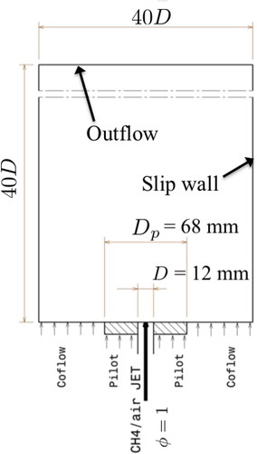
Three piloted stoichiometric methane-air Bunsen flames of Chen et al. (1996) considered in many past RANS (Amzin et al., 2012; Herrmann, 2006; Kolla and Swaminathan, 2010b; Lindstedt and Vaos, 2006; Prasad and Gore, 1999; Salehi and Bushe, 2010; Salehi et al., 2012; Stöllinger and Heinz, 2008, 2010) and LES (De and Acharya, 2009; Dodoulas and Navarro-Martinez, 2013; Langella et al., 2015; Pitsch and de Lagneste, 2002; Wang et al., 2011; Yilmaz et al., 2010) studies are chosen for this investigation. The reactant jet with a diameter of D = 12 mm issues into quiescent air and the flame is stabilized by laminar pilot flames of the same mixture. The pilot ring of a diameter D_p = 68 mm is water cooled and thus its burned mixture is sub-adiabatic. The turbulence in the reacting region is shear driven as there is no turbulence generating device in the reactant flow path. Three flames (F1, F2, and F3) with bulk mean velocity of U_b = 65, 50, and 35 m/s have a Reynolds number based on D and U_b of 52,000, 40,000, and 24,000, respectively, and this variation is achieved by changing only . The combustion conditions in these flames, as shown in Figure 1, are in the thin reaction zones regime and these conditions are calculated using the centerline values of turbulence RMS velocity, , and its integral length scale Λ = 2.4 mm near the nozzle exit reported by Chen et al. (1996). The Zeldovich thickness is , where v_u is the kinematic viscosity of the reactant mixture. The turbulent Reynolds number is defined as . The symbols D1 to D7 in Figure 1 denote the conditions of DNS flames used for a priori testing discussed in Section 6.1.

Figure 1. Combustion regime diagram showing conditions of flames F1, F2, and F3. The flames marked as D1 to D7 are DNS flames used for a priori model testing.

5. Simulation detail

The Favre filtered transport equations for conservation of mass and momentum are solved along with additional filtered equations required for combustion. The sub-grid stresses are modeled using the dynamic Smagorinsky model (Germano et al., 1991; Lilly, 1992) when is modeled using one of Eqs. (3) to (6) for the combustion part. A test-filter of size is employed for all dynamic procedures used here following the common practice, and the filter width is computed using the computational cell volume, V_i, as . If is modeled using then the sub-grid stresses are modeled as , with C_k computed dynamically (Germano et al., 1991).

The additional equations are for Favre filtered progress variable, , and total enthalpy, . The instantaneous c can be defined using absolute temperature, T, or a species mass fraction. Here, it is defined using the fuel mass fraction, Y_f, as so that it takes a value of 0 and 1 in the unburned and burned mixtures, respectively. This choice avoids a spurious flame that will appear numerically in the mixing layer between the pilot and coflow if c is defined using T or any other species mass fraction. The transport equation for is:

(10)

and the filtered reaction rate is closed using the models described in Section 2. One can also use a transport equation for instead of as there is no particular advantage in using either or for premixed combustion.

The governing equation for is:

(11)

Including this equation allows one to handle the sub-adiabatic pilot stream discussed in the previous section. The sub-grid scalar fluxes appearing in Eqs. (10) and (11) are computed using dynamic Schmidt number approach (Lilly, 1992).

The filtered temperature is obtained from using:

(12)

where K and is the specific heat capacity at constant pressure for the mixture, which depends on temperature as described by Ruan et al. (2014). The fluid mixture density is computed using the state equation where is the filtered pressure, is the Favre-filtered molecular mass of the mixture and R is the universal gas constant. The quantities , , and are specified through a lookup table constructed using planar unstrained laminar premixed flame of stoichiometric CH4-air mixture using CHEMKIN and GRI 3.0 mechanism with mixture averaged diffusivity formulation. The laminar solution is then convoluted using a Gaussian filter kernel with a width equal to the cube root of the smallest computational cell volume in LES. This table contains , , and filtered mass fractions of various species as a function of and is used during the LES. The LES statistics obtained using three times larger width for this filter kernel showed a negligible sensitivity of the statistics to this kernel width. Also, the use of an unstrained flamelet excludes the possible effects of fluid dynamic strain on filtered flame in LES, which will be explored in a future study.

A transport equation, similar to Eq. (11), for a passive fluid marker, , is included to account for the mixing or dilution of burned mixture with the entrained air. These effects were assessed to be important (Kolla and Swaminathan, 2010b) to capture the averaged values of various species mass fractions for , specifically for the F1 flame having the highest Reynolds number and thus this is included in this study. Briefly, the influence of entrained air is included using a mixing rule: (Kolla and Swaminathan, 2010b) where is a generic value representing or or or filtered mass fractions. The subscript ‘reac’ denotes that these values are taken from the lookup table for local and the subscript ‘air’ denotes their values in the air stream.

5.1. Numerical grid, boundary, and initial conditions

The filtered conservation and combustion modeling equations are solved using PRECISE-MB, which is based on a finite volume methodology (Anand et al., 1999). The spatial derivatives are discretized using a second-order central differencing scheme and the velocity-pressure coupling is achieved using the SIMPLEC algorithm (Doormaal and Raithby, 1984). The discretized equations are time advanced using a second-order accurate scheme with a constant time step and the CFL number is kept below 0.3 everywhere inside the computational domain spanning 40D in the axial and radial directions as shown in Figure 2, giving a total computational volume of π(40D)³/4. This volume is discretized using a structured multi-block grid having nonuniform numerical cells. These cells are fine near the burner exit and grow gradually in the downstream and radial directions. A coarse grid having 22 cells for D and about 4 cells within Λ measured at the jet exit gives a total of about 1.5 million cells for the computational volume considered. This grid has 404 cells in the streamwise direction along the centerline. Increasing the cell count to 32 for D and 6 for Λ keeping other grid parameters to be almost the same yields about 4.2 million cells in total. These two grids are used to assess the grid sensitivity of the LES statistics computed here. The coarse grid satisfies the 80% turbulent energy criterion of Pope (2000) and has the smallest normalized filter width and the fine grid has .

Figure 2. A schematic of the experimental (Chen et al., 1996) and computational setup of piloted stoichiometric methane-air Bunsen flames.

5.2. Boundary and initial conditions

The measured values at jet exit are used to specify the jet velocity and there is no velocity fluctuation specified at the exit as the turbulence is predominantly shear driven. A uniform velocity of 1.5m/s is specified for the pilot stream on the basis of the volumetric flow rate in the experiments. A small velocity of 0.2 m/s is assigned to the coflowing air to mimic the air entrainment and a 25% change to this velocity is observed to influence the LES statistics negligibly. The pilot temperature is unspecified in the experimental study and values ranging from 1785 to 2248 K were used in past studies (Amzin et al., 2012; De and Acharya, 2009; Dodoulas and Navarro-Martinez, 2013; Herrmann, 2006; Kolla and Swaminathan, 2010b; Lindstedt and Vaos, 2006; Pitsch and de Lagneste, 2002; Prasad and Gore, 1999; Salehi and Bushe, 2010; Salehi et al., 2012; Stöllinger and Heinz, 2008, 2010; Wang et al., 2011; Yilmaz et al., 2010) suggesting that the heat loss to the pilot burner varies from 0 (De and Acharya, 2009) to 34% (Dodoulas and Navarro-Martinez, 2013; Lindstedt and Vaos, 2006). A value of 17% was used by Herrmann (2006) and 20% heat loss was assumed by Pitsch and de Lagneste (2002) and Wang et al. (2011). For this study, it is taken to be 16% following Amzin et al. (2012) and Kolla and Swaminathan (2010b), which gives 1950 K for the pilot temperature. These past studies showed that this uncertainty influences the temperature only close to the jet exit (x ≤ 3D), which is also confirmed here by changing this temperature over a range of about 200 K.

The filtered progress variable is 0 in the jet exit and 1 for the pilot and coflowing streams. The passive fluid marker, , is 1 in the jet and pilot fluids and 0 in the coflowing air. The lateral boundaries are specified to be slip walls and the outlet has zero gradient in the streamwise direction for all of the variables.

The simulations are run using 96 cores running at 2.60 GHz, Intel Sandy Bridge E5-2670 processors on Darwin cluster at Cambridge University for about 0.15s to 0.25s of real flow time in total. The data are collected for about 32, 26, and 22 flow-through times for F1, F2, and F3 flames, respectively. The flow-through time is defined using the computational domain length and the respective U_b at the jet exit. These sampling times are substantially larger than what has been used typically in past studies for these flames and these simulations in the above cluster took about a day for 1.5M and two days for 4.2M grids on the wall clock.

6. Results and discussion

The details of DNS data used for a priori analyses are elaborated elsewhere (Gao et al., 2014) and thus only essential information required here is presented briefly. The DNS considered freely propagating turbulent premixed flames for a range of turbulence and thermochemical conditions given in Table 2 along with other relevant parameters defined as , . The Damköhler and Karlovitz numbers are and , respectively. The initial values of these parameters are given in Table 2 and the combustion conditions of DNS flames shown in Figure 1 are representative of those in the experimental flames. A single irreversible reaction with kinetic parameters representative of preheated methane-air combustion was used.

Table 2. Attributes of DNS flames.

Case		Λ^+	τ	Da	Ka	Ret
D1	5.00	1.67	4.5	0.33	8.67	22.0
D2	6.25	1.44	''	0.23	13.0	23.5
D3	7.50	2.50	''	0.33	''	49.0
D4	9.00	4.31	''	0.48	''	100.0
D5	11.25	3.75	''	0.33	19.5	110.0
D6	7.50	2.45	3.0	''	13.2	47.0
D7	''	''	4.5	''	''	''

The instantaneous quantities of interest are filtered using a Gaussian kernel with filter widths in the range of for a priori validation to be discussed next. The test filter width used for this analysis is as for the LES. More detail of the DNS data and their post-processing techniques can be found in Gao et al. (2014).

6.1. A priori analysis

6.1.1. model

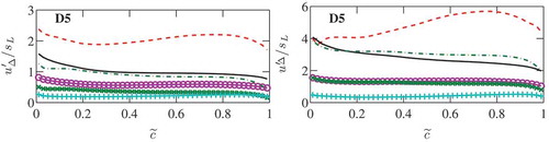
The SGS velocity is extracted directly from the DNS data using . The various quantities required to get through Eqs. (3) to (6) can also be extracted from the DNS data and thus these models can be verified by comparing their estimates to . These estimates are denoted as , or if Eq. (4) is used for modeling in the following discussion. Figure 3 compares the DNS results with modeled values across the filtered flame of the D5 case for two filter widths, and 2.8. These values of , shown in this figure, are obtained by averaging conditional on value. The D5 flame is shown because its combustion condition is akin to those in the experimental flames. The variation of shows that the SGS kinetic energy decreases across the flame and this trend does not depend on the filter widths used. As one would expect, the SGS kinetic energy level decreases as the filter width is decreased. All of these variations are captured by the standard models. The model in Eq. (6) predicts an increase in , which is expected for flames in the corrugated or wrinkled flamelets regime, but D5 is in the thin reaction zones regime as shown in Figure 1. Although the other models underpredict , with Eq. (5) giving the lowest value, their estimates are of the same order as the DNS result. The values estimated using Eq. (4) with C_q = 2.5 agree very well with the DNS results as shown in this figure, which suggests that the model parameter does not depend on the filter width. Furthermore, this analysis suggests that the modeling constants derived for nonreacting flows need to be revised for reacting flows, specifically for flames in the corrugated-flamelets regime (Langella et al., 2016). However, no such revision may be required for flames in the thin reaction zones regime because of stronger influence from turbulence compared to flame-induced effects on .

Figure 3. Comparison of (solid line) and its models—o: Eq. (3); ×: Eq. (4); +: Eq. (5); and dashed line: Eq. (6). The dash-dotted line is for Eq. (4) with C_q = 2.5. The results are shown for Δ⁺ = 0.8 (left) and 2.8 (right).

6.1.2. Effect of on and closures

The filtered dissipation can be rewritten as:

(13)

after averaging it over the DNS computational volume. This averaging operation is denoted by in the above equation. The typical variation of with Δ⁺ obtained from the DNS data is shown in Figure 4a. As one would expect approaches 1 when Δ⁺ goes towards zero implying that the SGS scalar dissipation rate, , is negligible. As Δ⁺ increases, the SGS contribution becomes substantial compared to the resolved component as has been observed in LES (Butz et al., 2015). This SGS contribution becomes about 50% and 2.5 times of the resolved part for Δ⁺ = 1.2 and Δ⁺ = 2.8, respectively. Thus, closure plays an important role for the filtered reaction rate calculation for large filter widths. The behavior of seen in Figure 4a is also suggestive of a power-law behavior as noted by Dunstan et al. (2013) and Gao et al. (2014), and further details can be found in these references.

Figure 4. Typical variation of (a) N with Δ⁺ and (b) with for Δ⁺ = 2.4. The DNS results (solid line) for case D5 are compared to the values obtained from the closure in Eq. (2) using (Δ) and [o: Eq. (3); ×: Eq. (4); +: Eq. (5); and □, dashed line in b: Eq. (6)].

Figure 4a also compares the DNS values with estimates obtained using various models discussed in Section 2. As one would expect, values obtained using agree well with its values obtained directly from the DNS, especially for large filter widths, demonstrating that Eq. (2) and its parameterization are very good as has been observed by Dunstan et al. (2013) and Gao et al. (2014). The error is observed to be about 24% for when Eqs. (3) or (4) are used and the error increases to about 27% for the scale similarity model of Bardina et al. (1980) in Eq. (5) when . The maximum error for the model based on the constant energy transfer hypothesis in Eq. (6) is about 10% suggesting that this model works well in an overall sense. A similar behavior is observed for other DNS flames listed in Table 2 also.

The influence of modeling on the local behavior of is shown in Figure 4b along with the values extracted directly from the DNS data. Although Figure 4a showed a good match between the DNS and modeled values of , there are some differences in when is used. The local variations obtained using Eq. (6) for follows closely the variation obtained using . The other three models for SGS velocity underestimate significantly, as seen in Figure 4b. This is consistent with the results shown in Figure 3. It is worth noting that C_q = 1 is used for Figure 4b and employing C_q = 2.5 would improve the model comparison, which can be verified quite easily using Eq. (2) with from Figure 3. However, the magnitude of this constant is observed not to influence LES results significantly.

The equation (2) can be written as:

(14)

where , after using . A direct influence of is through the linear term, which is also compounded by nonlinear effects coming through ka_Δ involved in C₃ and C₄. When the contributions from the second and third terms in Eq. (14) becomes very small. This behavior is expected because becomes very small under this condition and the unresolved dissipation rate is controlled by the thermochemical process. The SGS turbulence related term dominates when because and . The contributions from the terms involving C₃ and C₄ in Eq. (14) are of order unity for finite values of . The values of these two terms become about 0.38 and 0.13 for and they change to 0.10 and 0.23, respectively, for when . These estimates can change in a nonlinear manner with . However, the SGS turbulence level is linked to the filter width and so one cannot change these two parameters independently. Thus, the SGS velocity scale is expected to play a role in typical LES irrespective of the combustion regime. Furthermore, model will also influence the fluid dynamic field through the effects of heat release. Thus, one must be cautious in drawing conclusions from DNS analysis and extending them to LES without further testing.

Equation (1) can be used to show that the difference between the DNS and modeled filtered reaction rate is , which also holds for the volume averaged values. Thus, the differences between modeled and DNS values observed in Figure 4 apply for the filtered reaction rate also and a direct comparison is shown by Gao et al. (2014).

The above a priori assessments are conducted using β_c = 4, see Eqs. (2) and (14), for the case D5. This parameter takes a similar value [see Table 2 of Gao et al. (2014)] for other DNS cases and SGS dissipation rate obtained using this β_c obeys the realizability condition, . The β_c was shown to be influenced by τ (Gao et al., 2014) and thus its value for the experimental flames having τ = 6.4 can be quite different. Indeed, an extensive parametric testing using LES of F1, F2, and F3 flames suggests that for these flames, which is used for the LES results discussed next.

6.2. A posteriori analysis

The computational model used is a ssessed first using nonreacting flow results. The measurements of mean velocity and turbulent kinetic energy for a nonreacting jet are reported in Chen et al. (1996) for the conditions of the F2 flame. The LES results are time averaged first over the sampling period and then averaged in azimuthal direction in order to get radial variation of mean quantities at various axial positions, as has been done by Langella et al. (2015). This averaging procedure, which is also density weighted when required (Poinsot and Veynante, 2005), is denoted by using in the following discussion.

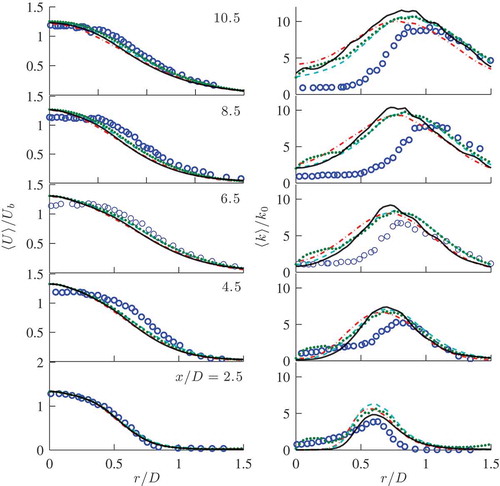
Figure 5 compares the computed and measured radial variations of averaged streamwise velocity and turbulent kinetic energy (TKE), , for five axial positions. The velocity is normalized using and the TKE is normalized using . The TKE is obtained as , where . The values of are obtained using Eq. (3) for the cold flow. The model in Eq. (6) was also used in the analysis but no significant difference was observed in the results.

The computed averaged streamwise velocity agrees very well with measurements as one sees in Figure 5 and the differences between 1.5M and 4.2M grid results are negligibly small. There are some differences between the computed and measured values of for r ≤ 0.55D, which decrease as one moves in the downstream direction (i.e., x > 6.5D). As seen in Figure 5, the turbulence levels represented by in regions of combustion (one shall see later that this would be r > 0.6D) are captured quite well. There is no turbulence specified at the jet exit and feeding some inlet turbulence improved the comparison of for x = 2.5D, but no significant changes were observed for other downstream locations because the turbulence is dominated by the shear generation mechanism in this flow configuration. It is clear from Figure 5 that the 1.5M grid is adequate to capture the flow dynamics and, hence, it is used for further analysis. Nevertheless, 4.2M grid is also used when required.

Figure 5. Comparison of measured (Chen et al., 1996) (symbols) and computed (lines) normalized mean axial velocity and turbulent kinetic energy in cold flow of flame F2. The radial variations are shown for five axial locations and two numerical grids, 1.5M (solid line) and 4.2M (dotted line).

6.2.1. Sensitivity of filtered reaction rate

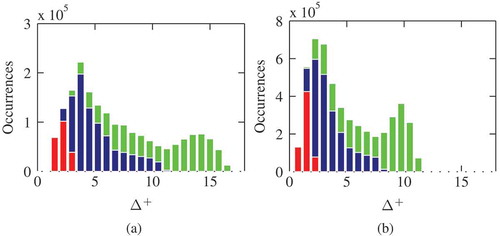
The normalized minimum filter sizes, , implied by the minimum cell volume are 1.3 and 0.8 for the 1.5M and 4.2M grids, respectively. These sizes become 2.8 and 1.7, respectively, if one uses the diagonal distance of the smallest grid. Since a spatially nonuniform grid is used, this width varies and typical distribution obtained using the local cell volume is shown in Figure 6 as a histogram for both the grids. This histogram is constructed using the grid information collected from the entire and two subparts of the computational domain having and , and and , where . The most likely width of the implied filter is about 2δ_th and 0.9δ_th for the 1.5M and 4.2M grids, respectively, for the smallest subdomain. When the subdomain size is increased the most likely and averaged widths are increased substantially, especially for the 1.5M grid. The most likely value of Δ⁺ is about 4 and the average value is about 5 to 6. There is a further increase in these values when the whole domain is considered for this analysis. The larger grid sizes near the lateral and outflow boundaries increase the count around and about 10, respectively, in Figures 6a and 6b. These Δ⁺ are substantially larger than what was typically used in past LES studies of these flames.

Figure 6. Histogram of normalized filter width, Δ⁺, for (a) 1.5M and (b) 4.2M grids. Different domain sizes are used for this plot: whole computational domain (green), 0 ≤ x ≤ 20D, 0 ≤ r ≤ 10D (blue), and 0 ≤ x ≤ 11D, 0 ≤ r ≤ 2D (red).

The influence of modeling on the filtered reaction rate computed in the LES is shown in Figure 7 for five models used in this study, as it is important to understand this sensitivity because the averaged reaction rate, thus the turbulent flame speed, will depend on this modeling for the algebraic reaction rate closure, Eq. (1), used in this study. The reaction rate is normalized using and the color map is shown for for an arbitrarily chosen time. The algebraic models in Eqs. (3) to (5) give relatively thinner fronts compared to that obtained using Eq. (6) or the equation. The flame length is more or less the same for all of the models and there is a slightly longer flame for the scale-similarity model in Eq. (4). Lilly’s model in Eq. (3) gives the shortest flame. Also, the peak reaction rate near the burner exit is seen only for Eq. 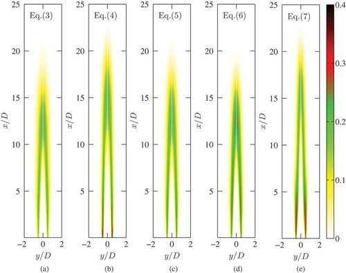(4) and transport equation. The peak reaction rate predicted by the other models is relatively smaller. The averaged normalized reaction rate shown in Figure 8 is almost similar for the various SGS velocity models. The difference is seen only in the region close to the jet exit (x ≤ 2.5D). The differences observed in Figures 7 and 8 suggest some sensitivity to modeling. It is not possible to do a quantitative analysis using reaction rate because this quantity is not reported in Chen et al. (1996) as it is not easy to measure it. However, one can make this assessment for overall performance of these models using statistics gathered from LES and measurements as has been done next.

Figure 7. Color map of normalized filtered reaction rate, , computed for various models.

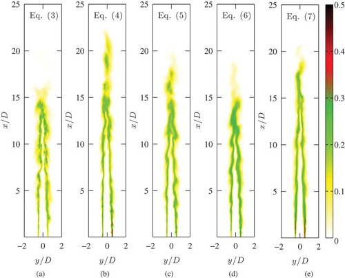
Figure 8. Color map of normalized mean reaction rate, , computed for various models.

6.2.2. Sensitivity of statistics

A priori analyses presented in Section 6.1 suggest that the sensitivity of LES statistics to modeling must be investigated. The flame F2 simulated using the 4.2M grid is chosen for this assessment because the results for the 1.5M grid is better than what is shown here and the results for the F1 and F3 flames are very similar.

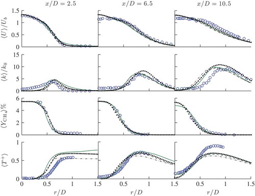
Figures 9 and 10 respectively show the sensitivities of fluid dynamic and scalar quantities to modeling. The radial variation of , is shown in Figure 9 for five streamwise locations. The averaged normalized TKE is also shown in this figure. The contribution of SGS kinetic energy to is obtained using the same model consistently for the four algebraic cases discussed in Section 2. The sensitivity of to the SGS velocity modeling is negligible whereas shows a weak sensitivity. All of the models overestimate for r ≤ 0.8D when x ≥ 8.5D and their estimates for the outer region, r > D, compare reasonably well with the measured values.

Figure 9. Influence of SGS velocity modeling on averaged streamwise velocity, , turbulent kinetic energy, for F2. Symbols (∘) are experimental results (Chen et al., 1996), lines are from simulations using Eq. (3) (

), Eq. (4) (

), Eq. (5) (

), and Eq. (6) (

).

The sensitivities of flame-related quantities, such as the fuel mass fraction and normalized temperature, are shown in Figure 10. The estimates of by the scale-similarity model in Eq. (4) are closer to the measured values. Although a similar behavior is seen for the normalized temperature there are some large underestimates for r > 0.7D, which is related to the performance of filtered reaction rate closure in Eq. (1) on 4.2M grid having Δ⁺< 1. The DNS analysis discussed in Section 6.1 suggests that this reaction rate closure underestimates the reaction rate for Δ < δ_th, which is also observed in LES (Langella et al., 2015). The results for the 1.5M grid discussed in Appendix B compares well with experimental data.

Figure 10. Influence of SGS velocity modeling on averaged fuel mass fraction and normalized temperature for F2. The legend is as for Figure 9.

Typical results obtained using the modeled equation, see Eq. (7), is shown in Figure 11 for the flame F2 along with the results obtained using Eq. (4). The influence of -based modeling on is negligible. The detail of the models K1, K2, and K3 are tabulated in Table 1. A similar behavior is observed for and the averaged fuel mass fraction shown respectively in the second and third rows of Figure 11. Although there are some small differences in the near field for the normalized averaged temperature, the differences become negligible for downstream locations as seen in the bottom row of Figure 11. From these results, one concludes that the results of -based modeling of are very similar to those of the scale-similarity model in Eq. (4). Thus, it does not seem to justify the additional computational effort required for transport equation. Furthermore, a negligible difference observed for the models K2 and K1 or K3 and K1 suggests that flame-generated turbulence included through Π in Eqs. (7) and (9) does not significantly influence the filtered reaction rate, thus the flame speed. Hence, the influence of flame on modeling can be neglected for the flames studied here. This is because these flames are in the thin reaction zones regime where the relatively high level of turbulence may mask the effects of flame-generated turbulence and this may not be so for flames in the corrugated flamelets regime as shown in Langella et al. (2016). However, one must acknowledge that the various sub-modeling for equation used here are ad hoc and further investigation is required to improve these models or to develop new ones.

Figure 11. Radial variations of normalized and averaged axial velocity, TKE, fuel mass fraction, and temperature in flame F2 obtained using SGS kinetic energy models: K1 (

), K2 (

), and K3 (

) are compared with measurements (Chen et al., 1996) (∘∘). The results obtained using the SGS velocity model in Eq. (4) are also shown above (

) for comparison.

Based on the above assessments, the scale-similarity model in Eq. (4) seems appropriate for the conditions of the flames investigated here. The models in Eqs. (3) and (5) are less satisfactory compared to those in Eqs. (4) and (6). Furthermore, it is to be noted that SGS stress-based models consider only the deviatoric part of this stress tensor and not the trace. Hence, it is debatable if one can use the stress-related models to get because the SGS kinetic energy per unit volume is related to the trace and so Eq. (4) is used for this study. It is possible to envisage that this model can be used for LES of flames over a wide range of combustion conditions. It is useful to understand the ability of the filtered reaction rate closure to capture the flame brush structure. Since the focus here is on the modeling sensitivity, the flame brush structure comparison is discussed in Appendix B for the sake of completeness of this investigation. These results show that the flame brush structure is captured quite well using the 1.5M grid, which is smaller than what was used in past studies.

7. Summary and conclusion

Large eddy simulations of piloted Bunsen flames of stoichiometric methane-air mixture are conducted. The filtered reaction rate is modeled using an algebraic closure involving scalar dissipation rate of reaction progress variable requiring a model for SGS velocity, . This closure belongs to the statistical category of flamelet modeling. Four algebraic models for are investigated along with a modeled transport equation for the SGS kinetic energy. Although some sensitivity of the SGS scalar dissipation rate, , and thus the filtered reaction rate, closure to the model is observed in a priori testing discussed in Section 6.1, the LES statistics show a weak sensitivity. The good agreement of flame brush structure computed using the algebraic closure for the filtered reaction rate, , along with the scale-similarity model, , suggests that these models work well for the flame conditions investigated in this study and also that ad hoc models accounting for flame-generated turbulence may not be required when the level of turbulence is relatively high as for the thin reaction zones regimes, which can explain the good comparisons shown in this study. However, the algebraic closure for the reaction rate does not include the finite rate chemistry and flame stretch effects. This closure also has one adjustable parameter, β_c, which can be evaluated dynamically as has been done by Langella et al. (2015) but a static value is used for this study to investigate the sensitivity to model without further complexity. Also, the β_c value used here is very close to the average of the values in the flame region obtained using the dynamic approach. The influences of flame stretch and finite rate chemistry can be included using either unstrained or strained flamelets as discussed in Langella and Swaminathan (2016).

Nomenclature

c	=	progress variable
Cm	=	combustion model parameter
Cp	=	specific heat capacity at constant pressure (kJ/kg-K)
CL, Cq,	=	SGS velocity modeling constants
Cs	=	Smagorinsky constant
	=	model constant for ɛk
	=	molecular diffusivity (m2/s)
D	=	jet diameter (m)
Dp	=	pilot diameter (m)
	=	factor in Eq. (2)
h	=	total enthalpy per mass unit (kJ/kg)
	=	enthalpy of formation per mass unit (kJ/kg)
	=	SGS kinetic energy per mass unit (m2/s)
k	=	turbulent kinetic energy per mass unit (m2/s2)
k0	=	centerline turbulent kinetic energy at inlet
	=	normalized filtered dissipation rate in Eq. (13)
Nc	=	scalar dissipation rate of c (1/s)
p	=	pressure (kJ/m3)
r	=	radial coordinate (m)
	=	universal gas constant (kJ/K-mol)
sL	=	laminar flame speed (m/s)
t	=	time (s)
T	=	temperature (K)
Ui	=	velocity component in direction i (m/s)
	=	velocity fluctuation in direction i (m/s)
	=	RMS velocity
	=	sub-grid scale velocity (m/s)
Ub	=	bulk velocity (m/s)
Vi	=	volume of cell i (m3)
W	=	molecular mass (kg/mol)
x, y, z	=	spacial coordinates (m)
Y	=	mass fraction
Da	=	Damköhler number
Ka	=	Karlovitz number
Re	=	Reynolds number

Greek symbols

α	=	thermal diffusivity (m2/s)
βc	=	combustion model parameter
δ	=	Zeldovich flame thickness (m)
δth	=	laminar flame thermal thickness (m)
Δ	=	filter width
	=	sub-grid scale scalar dissipation rate of c (1/s)
ɛk	=	dissipation of (m2/s3)
Λ	=	integral length scale (m)
µ	=	dynamic viscosity (kg/m-s)
v	=	kinematic viscosity (m2 s−1)
	=	pressure-dilatation term in Eq. (7)
ρ	=	density (kg/m3)
	=	variance of normalized T
τ	=	heat release parameter
	=	residual stress tensor (kg/m-s2)
	=	anisotropic part of
Ψ	=	passive fluid marker
	=	reaction rate (kg/m3-s)

Superscripts

+

=

variable normalized using laminar flame quantities

Subscripts

ad	=	adiabatic condition
Δ	=	sub-grid scale
f	=	fuel
L	=	laminar condition
min	=	minimum value in the domain
mix	=	mixture
reac	=	reaction (refers to flamelet condition)
t	=	turbulent or SGS
u	=	unburned condition

Operators

	=	simple filter of ϕ
	=	Favre filter of ϕ
	=	test filter of ϕ
	=	time or mass-weighted average of ϕ
	=	volume average of ϕ

Acronyms

CFL	=	Courant–Friedrichs–Lewy number
DNS	=	direct numerical simulation
LES	=	large eddy simulation
PDF	=	probability density function
RANS	=	Reynolds averaged Navier–Stokes
RMS	=	root mean square
URANS	=	unsteady RANS
SGS	=	sub-grid scale
TKE	=	turbulent kinetic energy

Acknowledgment

The authors gratefully acknowledge the support from EPSRC, Siemens, and Rolls-Royce.

Funding

This work is funded by the grant numbered EP/I027556/1.

Additional information

Funding

This work is funded by the grant numbered EP/I027556/1.

Appendix A: Strain rate based model for

If the energy transfer from large to filter scale is hypothesized to be constant, then for scale , one writes (Pope, 2000):

Also, if one takes and supposing that then:

(15)

The Smagorinsky model for v_t written as:

gives

(16)

Substituting Eq. (16) into Eq. (15) yields:

(17)

after some simple rearrangements and this equation is written as Eq. (6). This model allows one to relate SGS velocity fluctuation directly to the Smagorinsky model constant, and is strictly valid only when Eq. (15) holds. Although the assumption of seems too restrictive, the Smagorinsky model typically overestimates v_t and thus the above assumption is expected to be reasonable.

Appendix B: Analysis of flame brush structure

De and Acharya (2009) compared RANS and LES results for the experimental flames from a number of past studies and thus their results are used here for comparison. They used 1.88M and 5.91M cells in a domain of size 20D and 4D in the axial, x, and radial, r, directions, respectively, and their results using a modified thickened flame approach on the 1.88M grid is used here for comparison. The RANS-strained flamelets study of Kolla and Swaminathan (2010b) used an axisymmetric domain of x =7 0D and 45D in the axial and radial directions, respectively, with about a few hundred thousand cells. The LES-thickened flame study of Wang et al. (2011) used unstructured grids ranging from about 3.2M to 8.5M cells in a domain of size 120D ×120D. Their results from the 8.5M grid is used for comparison here. The recent LES-PDF study using Eulerian stochastic fields approach by Dodoulas and Navarro-Martinez (2013) used a computational domain of size 15D × 5D employing about 510k and 225k grids in the physical space and their results on their largest grid, and with 16 stochastic fields, is used here for comparison. Further detail on the combustion modeling and numerical methods used in these studies can be found in these references and the results available there are used for comparison.

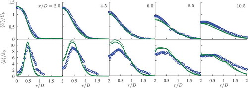
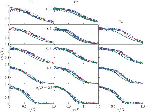
The radial variation of for various streamwise locations are shown in Figure B1 along with experimental measurements. Only two representative results from past studies are shown here because those results are very similar to one another. The current results are shown for the 1.5M grid and the results of the 4.2M grid are shown only for the F2 flame because the relative behavior is very similar for the other two flames. The difference in obtained using the 1.5M and 4.2M grids is negligibly small and the values obtained using the 1.5M grid compare well with the measurements also. These results agree well with those from past studies; however, a close examination of Figure B1 suggests that the agreement with the experimental data is better for the results of Wang et al. (2011), which used the 8.5M unstructured grid. Nevertheless, the difference among the numerical results and the data is observed to be small.

Figure B1. Comparison of radial variation of normalized axial velocity, , in experiments (Chen et al., 1996) (∘∘) and simulations (

) using the 1.5M grid. Results obtained using the 4.2M grid (

) are shown only for F2. Previous RANS (Kolla and Swaminathan, 2010b) (

) and LES (Wang et al., 2011) (

) results are also shown for comparison.

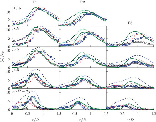
The radial variation of at various streamwise locations is shown in Figure B2 for the three flames. The LES results compare better with experimental data compared to previous RANS results as one would expect. The agreement between the measured and current computational values improves as the Reynolds number increases (going from F3 to F1), which is consistent with the general expectations for LES. The current results are in good agreement with the previous results as seen in Figure B2. However, the results of Wang et al. (2011) agree better with the data because they have used the 8.5M grid. The results obtained using the 4.2M grid agree quite well with the 1.5M results and the measurements for r ≥ 0.8D. The 4.2M grid results are good in general but an overprediction is seen for the inner region of the jet at downstream locations. Generally, second-order statistics such as TKE will have increased sensitivity to mesh resolution compared to first-order statistics as shown in Figure 19 of Wang et al. (2011). Thus, one would expect to see a better agreement for the 4.2M grid and the large difference seen here is because the combustion submodel in Eq. (1) is at its limit for this grid as noted earlier (see the discussion on Figures 4, 7, 8, 9, and 10). This SGS combustion model underestimates the reaction rate, heat release rate effects, and their interactions with turbulence as noted earlier for the 4.2M grid case. For these reasons, the 4.2M grid results will not be considered for the discussion below unless it is required otherwise.

Figure B2. Comparison of measured (Chen et al., 1996) (∘∘) and computed (

) variations with r/D. The computational results are for the 1.5M grid. Result of the 4.2M grid (

) is shown only for F2. Previous results De and Acharya (2009) and (Kolla and Swaminathan, 2010b) (

), and (Wang et al., 2011) (

) shown for comparison.

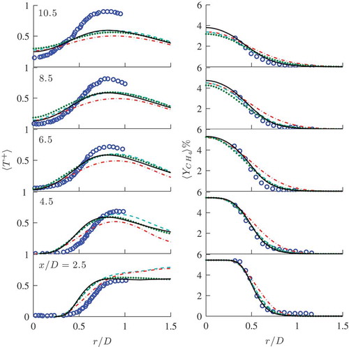
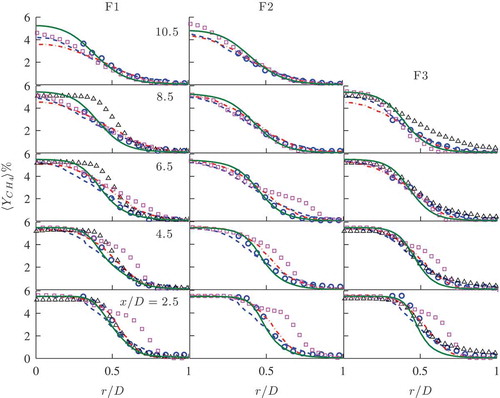
The radial variation of averaged fuel mass fraction is compared to the measured values in Figure B3. The results of previous numerical studies are also included in this figure. The thickened flame-LES results of De and Acharya (2009) agree very well with the measurements for for the high Da flame F3 and these computational results gradually move away from the experimental data as seen in this figure for the flame F1. However, the results of Wang et al. (2011) using a dynamic thickened flame approach show a good agreement uniformly. The agreement between the measured and computed values using the LES-PDF method (Dodoulas and Navarro-Martinez, 2013) is not uniformly good. The agreement is relatively better for x ≥ 8.5 for the flames F1 and F2, and for the flame F3 the agreement seems to improve from x = 6.5D as seen in Figure B3. It had been suggested that including the differential diffusion effects could improve these estimates for the LES-PDF method. The mean fuel mass fraction computed in this study using the flamelet-based algebraic model agrees very well with the measurements as shown in Figure B3.

Figure B3. The mean fuel mass fraction computed on the 1.5M grid (

) is compared to the measurements (Chen et al., 1996) (∘∘). Previous results (De and Acharya, 2009) (Δ), (Dodoulas and Navarro-Martinez, 2013) (□), (Kolla and Swaminathan, 2010b) (

), and (Wang et al., 2011) (

) are shown for comparison.

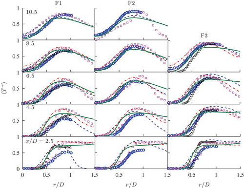
A similar comparison is shown in Figure B4 for the normalized temperature, . The values shown in Figures 10 and B4 are calculated as follows. First, the normalized filtered temperature is obtained using an expression proposed by Kolla and Swaminathan (2010b):

Figure B4. The mean normalized temperature computed on the 1.5M grid (

) is compared to the measurements (Chen et al., 1996) (∘∘). Previous results (De and Acharya, 2009) (Δ), (Dodoulas and Navarro-Martinez, 2013) (□), (Kolla and Swaminathan, 2010b) (

), and (Wang et al., 2011) (

) are shown for comparison.

(18)

where the RMS of normalized temperature fluctuation is obtained using and , where (Poinsot and Veynante, 2005). Strictly, one must also include the sub-grid variance, , while calculating and this SGS variance is unavailable in the modeling framework used here. A transport equation for needs to be solved to include the influences of reaction rate, dissipation rate, and turbulence on the evolution of this SGS variance and this will be considered in a future study.

Although one should use for comparison with measurements, no significant difference between and was observed for the flame conditions considered in this study. The flame F3 has the highest Damköhler number in the set and the computed values agree well with the data as shown in Figure B4. A very good agreement among various numerical studies is also observed for this flame. A large overestimate seen for the flame F1 for is because of the uncertainty in the pilot temperature, as it is not reported by Chen et al. (1996). Furthermore, the flame in the near field of the jet is expected to have quasi-laminar unsteady structure since the turbulence in these regions is low. The results in Figure B4 suggest that the compounded effects of these two factors (uncertainty and quasi-laminar unsteady flames) become more apparent as the turbulent Reynolds number increases (compare the difference between the computational and experimental values at x = 2.5D for all the three flames). The values of computed in this study agree well with the measurements at down stream locations as shown in the Figure B4. In general, a good agreement is observed for the statistics computed in this study with measurements.

The radial variations of averaged mass fractions of major, O₂, H₂O, and CO₂, and minor, OH, species and intermediates, H₂ and CO, are shown in Figures B5^{Figure B6Figure B7Figure B8}–B10 for various axial locations. The current statistics are also compared to past results available in the literature. A 2-step chemistry with empirical rate expression was used by De and Acharya (2009) and 1-step chemistry was used by Wang et al. (2011). The LES-PDF study by Dodoulas and Navarro-Martinez (2013) used a 4-step, 15-step, and GRI3.0 mechanisms and the results of the 15-step mechanism are used here. Because of these differences in the chemistry, a uniform comparison cannot be made for the various species.

Figure B5. Comparison of mean mass fraction of O₂: experimental data (Chen et al., 1996) (∘∘), present result (

), (De and Acharya, 2009) (Δ), Dodoulas and Navarro-Martinez (2013) (□), and (Kolla & Swaminathan, 2010b) (

). The dash-dotted line (

) for F1 at x/D = 2.5, 8.5, and 10.5 shows the value obtained without correcting for the dilution effects.

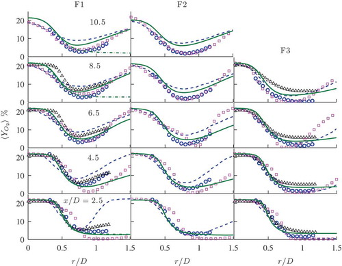
Figure B6. Comparison of mean mass fraction of H₂O: experimental data (Chen et al., 1996) (∘∘), present result (

), (De and Acharya, 2009) (Δ), (Dodoulas & Navarro-Martinez, 2013) (□), (Kolla and Swaminathan, 2010b) (

), and (Wang et al., 2011) (

).

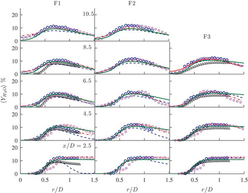
Figure B7. Comparison of mean mass fraction of CO₂: experimental data (Chen et al., 1996) (∘∘), present result (

), (De and Acharya, 2009) (Δ), (Dodoulas and Navarro-Martinez, 2013) (□), and (Kolla and Swaminathan, 2010b) (

).

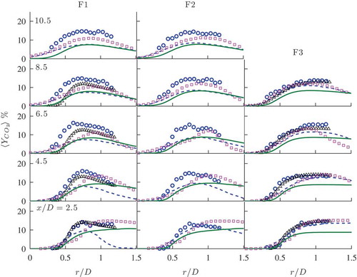
Figure B8. Comparison of mean mass fraction of OH: experimental data (Chen et al., 1996) (∘∘), present result (

), (Dodoulas and Navarro-Martinez, 2013) (□), and (Kolla and Swaminathan, 2010b) (

).

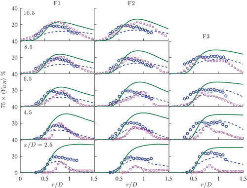
Figure B9. Comparison of mean mass fraction of H₂: experimental data (Chen et al., 1996) (∘∘), present result (

), and (Kolla and Swaminathan, 2010b) (

).

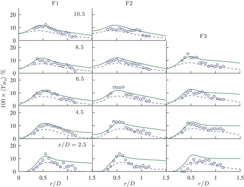
Figure B10. Comparison of mean mass fraction of CO: experimental data (Chen et al., 1996) (∘∘), present result (

), (De and Acharya, 2009) (Δ), (Dodoulas and Navarro-Martinez, 2013) (□), and (Kolla and Swaminathan, 2010b) (

).

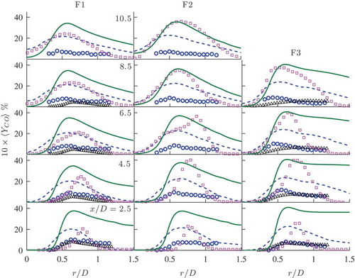
The mass fractions shown in these figures are obtained after correcting for the dilution effect as noted in Section 5, which is elucidated using the oxygen mass fraction at axial positions of x/D = 2.5, 8.5, and 10.5 for the flame F1. In the near field (x/D = 2.5), the influence of this effect is almost negligible and including this effect captures the oxygen mass fraction increase in the outer region, r > 0.8D, due to dilution with the air. The oxygen mass fraction computed using a 2-step chemistry and thickened flame model by De and Acharya (2009) is relatively larger compared to those obtained in the current study and those from the LES-PDF calculation by Dodoulas and Navarro-Martinez (2013). This difference increases with downstream distance. Wang et al. (2011) did not report O₂ and CO₂ mass fractions and thus they are not shown in Figures B5 and B7. The current results are improved over the previous RANS results as one would expect for the flames F1 and F2. This improvement is observed for H₂O, H₂, and OH. The averaged mass fraction of water vapor computed in this study agrees well with measured values and those reported in earlier LES studies. The underestimate seen for CO₂ mass fractions in Figure B7 is consistent with many earlier studies (De and Acharya, 2009; Dodoulas and Navarro-Martinez, 2013; Kolla and Swaminathan, 2010b) employing different combustion modeling approach. However, the values obtained using the LES-PDF method are relatively closer to the measurements for downstream locations. Although CO₂ is transported in the calculations reported by De and Acharya (2009) there is a large underestimate inside the flame brush for x ≥ 6.5D for the flame F1. For high Da flame F3, the computed CO₂ mass fractions agree well with the measured values. The OH mass fractions obtained using the LES-PDF (Dodoulas and Navarro-Martinez, 2013) and the current LES-flamelets methods agree quite well with one another and also with measurements for the flame F1. These agreements are relatively poor for upstream locations and for the largest Da flame F3 as shown in Figure B8. Nevertheless, the general trend is captured well by both of these modeling approaches.

The mean mass fraction of H₂ computed in this study agrees well with the measured values as shown in Figure B9. None of the previous LES studies reported this result and thus they are not included in this figure for comparison. The slight overestimate at x/D = 2.5 is because of the uncertainty in the pilot boundary condition and this uncertainty does not seem to be of any importance as one moves downstream.

The agreement for shown in Figure B10 is not good and there is a large overestimate for all three flames, which is consistent with the underestimate of CO₂ mass fraction. This could be related to the slow oxidation of CO, which may not be good for flamelet approach. However, a similar behavior is seen in Figure B10 for many previous studies using other combustion modeling techniques. This suggests that the reason may be somewhere else, perhaps in the measurement itself. Nevertheless, further analysis of the combustion model used in this study using other flame configurations and conditions is required. It is worth noting that, although the CO values computed by De and Acharya (2009) seem to agree quite well with the measurements, this seems to be inconsistent with their CO₂ values see Figure B7.

References

- Ahmed, I., and Swaminathan, N. 2013. Simulation of spherically expanding turbulent premixed flames. Combust. Sci. Technol. 185(10), 1509–1540.
- Ahmed, I., and Swaminathan, N. 2014. Simulation of turbulent explosion of hydrogen-air mixtures. Int. J. Hydrogen Energy, 39, 80–115.
- Amzin, S., and Swaminathan, N. 2013. Computations of turbulent lean premixed combustion using cmc. Combust. Theor. Model., 17(6), 1125–1153.
- Amzin, S., Swaminathan, N., Rogerson, J.W., and Kent, J.H. 2012. Conditional moment closure for turbulent premixed flames. Combust. Sci. Technol., 184(10–11), 1743–1767.
- Anand, M.S., Zhu, J., Connor, C., and Razdan, M. 1999. Combustor flow analysis using an advanced finite-volume design system. In International Gas Turbine and Aeroengine Congress and Exhibition, ASME, Indianapolis, Vol. 99-GT, p. 273.
- Bardina, J., Ferziger, J.H., and Reynolds, W.C. 1980. Improved subgrid scale models for large-eddy simulation. Am. Inst. Aeronaut. Astronaut., 80, 1357.
- Boger, M., Veynante, D., Boughanem, H., and Trouvé, A. 1998. Direct numerical simulation analysis of flame surface density concept for large eddy simulation of turbulent premixed combustion. Proc. Combust. Inst., 27, 917–925.
- Bray, K.N.C. 1979. The interaction between turbulence and combustion. Proc. Combust. Inst., 17, 223–233.
- Bray, K.N.C. 1980. Turbulent flows with premixed reactants. In P.A. Libby and F.A. Williams, (Eds.), Turbulent Reacting Flows, Springer-Verlag, New York, pp. 115–183.
- Bulat, G., Jones, W.P., and Marquis, A.J. 2014. NO and CO formation in an industrial gas-turbine combustion chamber using LES with the Eulerian sub-grid PDF method. Combust. Flame, 161(7), 1804–1825.
- Butz, D., Gao, Y., Kempf, A.M., and Chakraborty, N. 2015. Large eddy simulations of a turbulent premixed swirl flame using an algebraic scalar dissipation rate closure. Combust. Flame, 162(9), 3180–3196.
- Cant, R.S. 2011. RANS and LES modelling of turbulent combustion. In T. Echekki and E. Mastorakos, Turbulent Combustion Modelling: Advances, New Trends and Perspectives, Springer, Heidelberg, pp. 63–87.
- Chai, X., and Mahesh, K. 2012. Dynamic K-equation model for large eddy simulation of compressible flow. J. Fluid Mech., 699, 385–413.
- Chakraborty, N., and Cant, R.S. 2007. A priori analysis of the curvature and propagation terms of the flame surface density transport equation for large eddy simulation. Phys. Fluids, 19, 105101.
- Chakraborty, N., and Cant, R.S. 2011. Effects of Lewis number on flame surface density transport in turbulent premixed combustion. Combust. Flame, 158, 1768–1787.
- Chakraborty, N., and Klein, M. 2008. A priori direct numerical simulation assessment of algebraic flame surface density models for turbulent premixed flames in the context of large eddy simulation. Phys. Fluids, 20, 085108.
- Chakraborty, N., Rogerson, J.W., and Swaminathan, N. 2008. A priori assessment of closures for scalar dissipation rate transport in turbulent premixed flames using direct numerical simulation. Phys. Fluids, 20, 045106.
- Chakraborty, N., and Swaminathan, N. 2007. Influence of the Damköhler number on turbulence-scalar interaction in premixed flames. II. Model development. Phys. Fluids, 19, 045104–1–11.
- Chakraborty, N., and Swaminathan, N. 2011. Effects of Lewis number on scalar variance transport in premixed flames. Flow Turbul. Combust., 87, 261–292.
- Chen, Y.-C., Peters, N., Schneemann, G.A., Wruck, N., Renz, U. and Mansour, M.S. 1996. The detailed structure of highly stretched turbulent premixed methane-air flames. Combust. Flame, 107, 223–244.
- Colin, O., Ducros, F., Veynante, D., and Poinsot, T.J. 2000. A thickened flame model for large eddy simulations of turbulent premixed combustion. Phys. Fluids, 12, 1843.
- De, A., and Acharya, S. 2009. Large eddy simulation of a premixed Bunsen flame using a modified thickened-flame model at two Reynolds number. Proc. Combust. Inst., 181(10), 1231–1272.
- Deardorff, J.W. 1974. Three-dimensional numerical study of the height and mean structure of a heated planetary boundary layer. Boundary Layer Meteorol., 7, 81–106.
- Dodoulas, I.A. and Navarro-Martinez, S. 2013. Large eddy simulation of premixed turbulent flames using the probability density function approach. Flow Turbul. Combust., 90, 645–678.
- Doormaal, J.P. Van and Raithby, G.D. 1984. Enhancements of the simple method for predicting incompressible fluid flows. Numer. Heat Transfer, 7(2), 147–163.
- Dunstan, T. D., Minamoto, Y., Chakraborty, N., and Swaminathan, N. 2013. Scalar dissipation rate modelling for large eddy simulation of turbulent premixed flames. Proc. Combust. Inst., 34, 1193–1201.
- Ferziger, J.H. 1997. Large eddy simulation: An introduction and perspective. In O. Métais and J.H. Ferziger, Eds., New Tools in Turbulence Modelling, Springer-Verlag, Berlin Heidelberg, pp. 29–47.
- Gao, Y., Chakraborty, N., and Swaminathan, N. 2014. Algebraic closure of scalar dissipation rate for large eddy simulations of turbulent premixed combustion. Combust. Sci. Technol., 186(10–11), 1309–1337.
- Germano, M., Piomelli, U., Moin, P., and Cabot, W.H. 1991. A dynamic subgrid-scale eddy viscosity model. Phys. Fluids A, 3(7), 1760.
- Gicquel, L.Y.M., Staffelbach, G., and Poinsot, T. 2012. Large eddy simulations of gaseous flames in gas turbine combustion chambers. Prog. Energy Combust. Sci., 38, 782–817.
- Gubba, S.R., Ibrahim, S.S. and Malalasekera, W. 2012. Dynamic flame surface density modelling of flame deflagration in vented explosion. Combust. Explor. Shock Waves, 48, 393–405.
- Hawkes, E.R., and Cant, R.S. 2001. Implications of a flame surface density approach to large eddy simulation of premixed turbulent combustion. Combust. Flame, 126, 1617–1629.
- Herrmann, M. 2006. Numerical simulation of turbulent bunsen flames with a level set flamelet model. Combust. Flame, 145, 357–375.
- Klimenko, A. Yu., and Bilger, R.W. 1999. Conditional moment closure for turbulent combustion. Prog. Energy Combust. Sci., 25(6), 595–687.
- Knikker, R., Veynante, D., and Meneveau, C. 2004. A dynamic flame surface density model for large eddy simulations of turbulent premixed combustion. Phys. Fluids, 16, 91.
- Kolla, H., Rogerson, J.W., Chakraborty, N., and Swaminathan, N. 2009. Scalar dissipation rate modeling and its validation. Combust. Sci. Technol., 181, 518–535.
- Kolla, H., and Swaminathan, N. 2010a. Strained flamelets for turbulent premixed flames, i: Formulation and planar flame results. Combust. Flame, 157, 943–954.
- Kolla, H., and Swaminathan, N. 2010b. Strained flamelets for turbulent premixed flames. II: Laboratory flame results. Combust. Flame, 157, 1274–1289.
- Langella, I., and Swaminathan, N. 2016. Unstrained and strained flamelets for LES of premixed combustion. Combust. Theor. Model, 20(3), 410–440.
- Langella, I., Swaminathan, N., Gao, Y., and Chakraborty, N. 2015. Assessment of dynamic closure for premixed combustion LES. Combust. Theor Model. 19(5), 628–656.
- Langella, I., Swaminathan, N., Williams, F.A., and Furukawa, J. 2016. Large-eddy simulation of premixed combustion in the corrugated-flamelet regime. Combust. Sci. Technol., 188(9), 1565–1591.
- Lilly, D.K. 1992. A proposed modification of the germano subgrid scale closure method. Phys. Fluids A, 4, 633–635.
- Lilly, D.K. 1966. On the application of the eddy viscosity concept in the inertial sub-range of turbulence. Technical Report 123. NCAR, Boulder, CO.
- Lilly, D. K. 1967. The representation of small-scale turbulence in numerical simulation experiments. In H.H Goldstine, Ed., Proceedings of the IBM Scientific Computing Symposium on Environmental Sciences, IBM, Yorktown Heights, NY, pp. 195–210.
- Lindstedt, R.P. and Vaos, E.M. 2006. Transported PDF modeling of high-Reynolds-number premixed turbulent flames. Combust. Flame, 145, 495–511.
- Liu, S., Meneveau, C., and Katz, J. 1994. Similarity subgrid-scale models as deduced from measurements in a turbulent jet. J. Fluid Mech., 215, 83–119.
- Ma, T., Gao, Y., Kempf, A.M., and Chakraborty, N. 2014. Validation and implementation of algebraic LES modelling of scalar dissipation rate for reaction rate closure in turbulent premixed combustion. Combust. Flame, 161, 3134–3153.
- Martin, S.M., Kramlich, J.C., Kosaly, G., and Riley, J.J. 2003. The premixed conditional moment closure method applied to idealized lean premixed gas turbine combustors. J. Eng. Gas Turbines. Power, 125(4), 895–900.
- Moureau, V., Fiorina, B., and Pitsch, H. 2008. A level set formulation for premixed combustion LES considering the turbulent flame structure. Combust. Flame, 156(4), 801–812.
- Pitsch, H. 2005. A consistent level set formulation for large-eddy simulation of premixed turbulent combustion. Combust. Flame, 143(4), 587–598.
- Pitsch, H. 2006. Large-eddy simulation of turbulent combustion. Annu. Rev. Fluid Mech., 38, 453–482.
- Pitsch, H., and de Lagneste, L.D. 2002. Large-eddy simulation of a premixed turbulent combustion using level-set approach. Proc. Combust. Inst., 29, 2001–2208.
- Poinsot, T.J., and Veynante, D. 2005. Theoretical and Numerical Combustion, R.T. Edwards Inc., Flourtown, PA.
- Pope, S.B. 2000. Turbulent Flows, Cambridge University Press, Cambridge, UK.
- Prasad, R.O.S., and Gore, J.P. 1999. An evaluation of flame surface density models for turbulent premixed jet flames. Combust. Flame, 116, 1–14.
- Rowinski, D.H., and Pope, S.B. 2013. Computational study of lean premixed turbulent flames using ranspdf and lespdf methods. Combust. Theor. Model., 17(4), 610–656.
- Ruan, S., Swaminathan, N., and Darbyshire, O. 2014. Modelling of turbulent lifted jet flames using flamelets: A priori assessment and a posteriori validation. Combust. Theor. Model. 18(2), 295–329.
- Salehi, M., and Bushe, W. 2010. Presumed PDF modelling for RANS simulation of turbulent premixed flames. Combust. Theor. Model., 14(3), 381–403.
- Salehi, M., Bushe, W., and Daun, K. 2012. Application of the conditional source term estimation for turbulence chemistry interactions in a premixed flame. Combust. Theor. Model., 16(2), 301–320.
- Schumann, U. 1975. Subgrid scale model for finite difference simulations of turbulent flows in plane channels and annuli. J. Comput. Phys., 18, 374–404.
- Smagorinsky, J. 1963. General circulation experiments with the primitive equations. I. The basic experiment. Mon. Weather Rev., 91(3), 99–164.
- Stöllinger, M., and Heinz, S. 2008. PDF modelling and simulation of premixed turbulent combustion. Monte Carlo Methods Appl., 14(4), 343–377.
- Stöllinger, M., and Heinz, S. 2010. Evaluation of scalar mixing and time scale models in PDF simulations of a turbulent premixed flame. Combust. Flame, 157(9), 1671–1685.
- Swaminathan, N., and Bray, K.N.C. 2011. Fundamentals and challenges. In N. Swaminathan and K.N.C Bray, Eds., Turbulent Premixed Flames, Cambridge University Press, Cambridge, UK, pp. 1–40.
- Swaminathan, N., Xu, G., Dowling, A.P. and Balachandran, R. 2012. Heat release rate correlation and combustion noise in premixed flames. J. Fluid Mech., 681, 80–115.
- Wang, G., Boileau, M., and Veynante, D. 2011. Implementation of a dynamic thickened flame model for large eddy simulations of turbulent premixed combustion. Combust. Flame, 158, 2199–2213.
- Wang, G., Boileau, M., Veynante, D., and Truffin, K. 2012. Large eddy simulation of a growing turbulent premixed flame kernel using a dynamic flame surface density model. Combust. Flame, 159(8), 2742–2754.
- Yilmaz, S.L., Nik, M.B., Givi, P., and Strakey, P.A. 2010. Scalar filtered density function for large eddy simulation of a Bunsen burner. J. Propul. Power, 26(1), 84–93.