A Fractal Dynamic SGS Combustion Model for Large Eddy Simulation of Turbulent Premixed Flames

ABSTRACT

Direct numerical simulation of a turbulent hydrogen-air premixed plane jet flame is performed to investigate fractal characteristics and to evaluate the fractal dynamic subgrid scale (FDSGS) combustion model. The DNS results show that the fractal dimension of flame surfaces increases with the downstream distance, and the fractal dimension computed using a 3D box-counting method reaches about 2.54 in the region where turbulence is developed by mean shear. An inner cutoff representation employed in the FDSGS combustion model could be used in large eddy simulations (LES) of complicated combustion problems. Static tests show that the procedure applied in the FDSGS combustion model adequately predicts the fractal dimension, Kolmogorov length scale, and flame surface area despite the presence of strong mean shear. Dynamic model evaluations are also carried out by conducting a series of LES using the FDSGS and other combustion models. In the dynamic tests, the mean temperature distributions and peak positions of variations of a reaction progress variable fluctuation in the transverse direction obtained from the LES with the FDSGS combustion model show good agreement with the filtered DNS fields. The present evaluation also revealed that one of the strengths in the FDSGS combustion modeling approach is that the model does not require SGS turbulent velocity fluctuation, since modeling of this quantity is straightforward for neither homogeneous turbulence nor the turbulent shear flows.

KEYWORDS:

• Fractal characteristics
• Large eddy simulation
• Subgrid scale combustion model
• Turbulent premixed flame
• Turbulent shear flow

Introduction

Large eddy simulation (LES) is a promising tool for design of combustion devices since it requires realistic computational resources in general while resolving large scale unsteady fluid and flame motions. Studies on the LES of turbulent premixed combustion in real industrial burners and existing engines were reviewed by Gicquel et al. (2012). In LES, physical quantities are filtered and divided into grid scale (GS) and subgrid scale (SGS) components. In LES of turbulent premixed combustion, an SGS combustion model is required to compute additional terms associated with filtered transport equations for reacting scalars. In modeling for LES, the key challenges are to describe interaction between unresolved flame structures and eddy structures in turbulence, and to track flame fronts propagating in the turbulence. Such interactions are often modeled based on the assumption that flame thickness is generally quite thin compared to the GS (i.e., LES filter width ) (Peters, 2000) since the filter width is relevant to the inertial subrange of turbulence. There are several approaches for the unclosed LES transport equations that are summarized in several reviews (Haworth, 2010; Pitsch, 2006; Veynante and Vervisch, 2002), and prediction of filtered reaction rate or flame propagation speed is required in the most of the approaches except transported PDF and conditional moment closure-type approach (Kim and Pope, 2014; Thornber et al., 2011). Among them, flame surface area is one of the important quantities that is used for SGS combustion models in several LES approaches. Applying Damköhler’s hypothesis (Damköhler, 1940), which assumes that a turbulent flame front is infinitely thin, a turbulent flame speed may be expressed using a laminar flame speed and the ratio of turbulent and laminar flame surface areas in GS as:

(1)

The turbulent flame speed is explicitly appears in the level-set approach to close so-called filtered -equation (Peters, 2000; Pitsch, 2002). The same flame surface area ratio is also used for one of the reaction rate modeling approaches of filtered reactive scalar transport equation. In the transport equation of a reaction progress variable , a flame wrinkling factor is the key parameter and it may be computed as (Charlette et al., 2002a), where denotes the filtered value of a quantity . Therefore, modelling the flame surface area of turbulent premixed flames in GS is of the primary interest in the present study.

One approach to obtain the turbulent flame surface area for SGS combustion models is based on fractal characteristics (Chakraborty and Klein, 2008; Charlette et al., 2002a; Chatakonda et al., 2010; Fureby, 2005; Gouldin, 1987; Gülder, 1990; Knikker et al., 2004; Yoshikawa et al., 2013). The fractal characteristics have been investigated in many studies (Cohé et al., 2007; Gülder and Smallwood, 1995; Kobayashi and Kawazoe, 2000; Mantzaras, 1992; Peters, 1986; Poinsot et al., 1990; Shim et al., 2011). Kobayashi and Kawazoe (2000) investigated the fractal characteristics of turbulent premixed flames in a high pressure combustion chamber and reported the fractal dimensions between 2.1 and 2.3. Cintosun et al. (2007) shows that the fractal dimensions of turbulent premixed Bunsen-type burners are in the range from 2.15–2.45 depending on fractal analysis methods. Several inner cutoff expressions have been proposed based on the Karlovitz number (Gülder and Smallwood, 1995; Peters, 1986; Poinsot et al., 1990; Roberts et al., 1993), normalized turbulent intensity and Karlovitz number (Mantzaras, 1992) and the most expected diameter of coherent fine scale eddies (Shim et al., 2011). Although there is no consensus on fractal characteristics in turbulent premixed combustion, several SGS combustion models have been developed based on the insights obtained so far (Chakraborty and Klein, 2008; Charlette et al., 2002a, 2002b; Chatakonda et al., 2010; Fureby, 2005; Gouldin, 1987; Gülder, 1990; Knikker et al., 2004; Yoshikawa et al., 2013). Charlette et al. (2002b) and Knikker et al. (2004) developed dynamic determination procedures of the fractal dimension, while Fureby (2005), Chakraborty and Klein (2008), and Chatakonda et al. (2010) introduced empirical fitting functions. Chakraborty and Klein (2008) and Chatakonda et al. (2010) used correlating equations for the inner cutoff. Charlette et al. (2002a) and Fureby (2005) related the inner cutoff with an efficiency function for net strain effect on flame.

In a previous study (Yoshikawa et al., 2013), a fractal dynamic SGS (FDSGS) combustion model was proposed for the prediction of flame surface area in the context of the level set approach. They performed static tests with DNS data of hydrogen–air premixed flames freely propagating in a homogeneous turbulence to evaluate the FDSGS combustion model. The combustion model has shown a good performance overall in the combustion configuration. However, mean velocity shear exists in turbulent premixed flames in practical combustion devices and they influence turbulence–flame interaction characteristics significantly (Minamoto et al., 2011). Thus, several physical quantities relevant to this model, such as fractal dimension, and inner cutoff, need to be studied and the model performance should be thoroughly verified in such a configuration.

For these purposes, fractal characteristics in shear layers are first investigated using the direct numerical simulation (DNS) of a turbulent premixed jet flame. Afterwards, a priori tests are carried out using the same DNS data sets to evaluate the overall performance of the FDSGS combustion model. LES with a turbulent combustion configuration the same as the turbulent jet premixed flame DNS is also performed using the combustion model with different numerical parameters to compare the LES solutions directly with the filtered DNS results. For comparison, other SGS combustion models are also tested.

This article first describes the mathematical background of the FDSGS combustion model. Then, DNS methodology and the conditions considered in this study are explained, before discussing the fractal characteristics of the turbulent combustion field exposed to strong shear layers. In the final two sections, the FDSGS combustion model is evaluated by means of a priori and a posteriori analysis by conducting LES using the same configuration and condition as the DNS.

Fractal dynamic SGS combustion model

In this section, the derivation of the FDSGS combustion model is described (Yoshikawa et al., 2013). The model predicts the ratio of turbulent and laminar flame surface areas in GS, which is based on the fractal characteristics that are analysed and discussed later in the section “Fractal Characteristics.” As explained in this section, there are three key quantities for the FDSGS combustion model: (1) fractal dimension, (2) inner cutoff, and (3) Kolmogorov length scale; the methods to obtain these quantities from filtered fields are also explained later in this section.

In the present model, the flame surface area ratio is expressed as the sum of two terms that represent turbulence and dilatation contributions on the flame surface area in SGS, respectively denoted as and in Eq. (2). The first term relevant to the turbulence effect is modeled in the context of the fractal characteristics of turbulent premixed flame surfaces and scale separation of high Reynolds number turbulence, while the other term is based on dilatation of one-dimensional flamelets.

(2)

where denotes the filter width of LES. Flame surface area can be expressed with the fractal dimension , the inner cutoff , and outer cutoff. Given that the outer cutoff is similar to and that the inner cutoff is scaled by the Kolmogorov length scale (Shim et al., 2011), the turbulence contribution to the flame surface area may be written as:

(3)

where is a scaling factor given by a correlation equation between the inner cutoff and the most expected diameter of coherent fine scale eddies, , (Shim et al., 2011; Tanahashi et al., 2001):

(4)

Here, is a model constant , and represents the Zel’dovich flame thickness computed as . Equations (4) and (3) have two quantities, and , that have to be indirectly computed during LES. For modeling the Kolmogorov length scale, scale separation of turbulence (i.e., in high Reynolds number flows, where and are the integral length scale and the Taylor micro-scale) is assumed. Since the LES filter width is of the order of the integral length scale, most of turbulent kinetic energy dissipates in SGS (i.e., , where and are turbulent kinetic energy dissipation rate and its SGS portion). Assuming the local equilibrium of the energy production and the energy dissipation rate at SGS , and applying the Smagorinsky model to SGS Reynolds stress, is expressed as:

(5)

where , and are the SGS stress tensor, strain rate tensor, and Smagorinsky constant, respectively, and denotes the Favre filtered value of a quantity . The strain rate is caused by both the turbulence motion and the dilation of the fluid due to the heat release. Since the turbulence effect alone is considered to calculate for , the dilatation effect is subtracted from the strain rate tensor in Eq. (5). Using Eq. (5), the Kolmovorov length scale is given as

(6)

Here, has the value at the temperature of the unburned mixture. From Eqs. (3) and (6), the turbulence effect on the flame surface area is modeled as

(7)

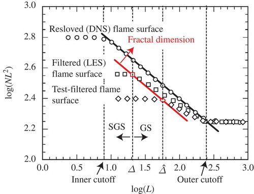
The last unknown in Eq. (3), fractal dimension , is dynamically computed during LES using the procedure reported in Miyauchi et al. (1994) as follows. First, box-counting is performed for LES flame surfaces at grid scale, , and for test-filtered flame surfaces at larger test-filter scale, . Then the fractal dimension is straightforwardly obtained using these two information as in the schematic in Figure 1. The dynamic procedure is locally applied in cubic control volumes (CVs) in the LES domain. The size of CV is set to or in edge length in the present study. This procedure is repeated every iteration to include temporal variation of the characteristics.

Figure 1. A schematic of variations of counted boxes at different box sizes to be used for the FDSGS approach.

The dilatation contribution mentioned in Eq. (2) is separately modeled based on the flamelet concept. Assuming local 1D laminar flames, dilatation is expressed as , where the subscript denotes flame normal direction. The volume integral of dilatation in a control volume without turbulence effect represented by GS of LES is approximated as:

(8)

Here, the subscript th represents the values in a laminar flame and is the thermal thickness of the corresponding laminar flame computed based on the maximum temperature gradient. The subscript F₀ denotes a value to be used to identify flame surface defined based on either or . The symbol represents a pseudo flame thickness of a filtered laminar flame expressed as:

(9)

Using the relation in Eq. (8), the dilatation contribution to the flame surface area is modeled as:

(10)

The ratio of turbulent and laminar flame surface areas is computed as the sum of Eqs. (7) and (10) as in Eq. (2). Any terms appearing in the present model (in Eqs. (7) and (10)) are not based on the estimation of the SGS turbulent velocity fluctuation explicitly or implicitly. This is an important aspect of the present modeling approach and is the major difference from other approaches (Chakraborty and Klein, 2008; Charlette et al., 2002a; Chatakonda et al., 2010; Colin et al., 2000; Flohr and Pitsch, 2000; Fureby, 2005; Gülder, 1990; Knikker et al., 2004; Pitsch and Duchamp De Lageneste, 2002).

DNS of a turbulent premixed plane jet flame

For the purposes of fractal analysis and FDSGS combustion model validation using a priori and posteriori testing, DNS is performed for a H₂-air premixed plane jet flame (Shimura et al., 2012). The DNS solves fully compressible governing equations for mass, momentum, energy, and mass fractions of chemical species. In the DNS, Soret effect, Dufour effect, pressure gradient diffusion, bulk viscosity, and radiative heat transfer are assumed to be negligible, which is a standard practice. The H-air combustion chemistry is modeled using a detailed kinetic mechanism consisting of 12 reactive species (, , , , , , , , , , and ) and 27 elementary reactions (Gutheil et al., 1993). The temperature dependence of the viscosity, the thermal conductivity, and the diffusion coefficients are also taken into account. The governing equations are spatially discretized using fourth order finite central difference scheme, and the same order compact finite difference filter (Lele, 1992) is applied to eliminate numerical oscillations with higher frequency than spatial resolution of the finite difference scheme. Time integration is achieved by third-order Runge–Kutta scheme. Since the use of detailed chemistry results in a stiff problem, a point implicit method with VODE solver (Brown et al., 1989) is applied for chemical source terms. The DNS configuration is shown in Figure 2. The H₂-air premixed reactants are issued from the jet inflow surrounded by co-flow streams that consists of burned gas. Inflow and non-reflecting outflow boundaries are applied based on Navier–Stokes characteristic boundary conditions (NSCBC) (Baum et al., 1994; Poinsot and Lele, 1992) in and directions and periodic boundary in z direction. The dimensions of computational domain are . The domain is discretized using 1281 × 1025 × 513 mesh points, which ensures mesh points within the flame thermal thickness . The mean inflow velocity is given by combining two hyperbolic tangent velocity profiles:

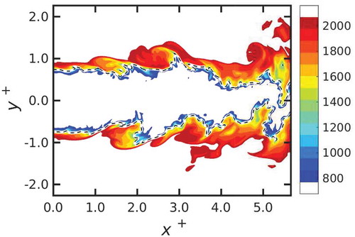
Figure 2. DNS configuration and simulated flame. Red iso-surfaces: , cyan iso-surfaces: the second invariant .

(11)

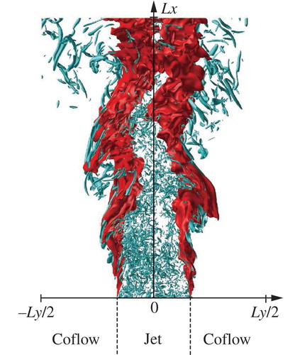
The vorticity thickness, , is set to be 0.5 mm, where . Most unstable wavelength of the present inflow velocity is (Michalke, 1964). The mean inflow velocities of the reactants (jet, ) and the products (co-flow, ) are set to be 350 m/s and 20 m/s, respectively. This gives a mean flow-through time (mean jet convection time from the inflow to outflow boundaries) of s. Any lengths, times, and velocities normalized using , , and are denoted by the superscript “+” later. Equivalence ratio, temperature, and pressure of the reactant mixture are set to be 1.0, 700 K, and 0.1 MPa, respectively.

Fully developed homogeneous isotropic turbulence (HIT) simulated in a preliminary DNS is superimposed onto the mean inflow velocity of the unburnted mixture as velocity fluctuations, whose important parameters are described later in this section. The DNS domain is initialized using the same method as the inflow. After the initialization, the simulation was run for 1.2 flow-through times until initial transients left. The simulation is continued for additional flow-through times, and six snapshots are collected for analysis.

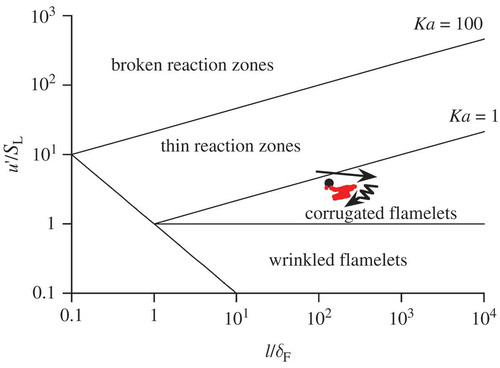
The inflow turbulence parameters of the HIT issued from the inflow boundary are as follows: Reynolds number based on , ; that based on , ; mm; mm; m; turbulent intensity m/s. The corresponding laminar flame parameters are m/s, mm, and m. Based on these quantities, the turbulent combustion condition is located close to the boundary between the corrugated flamelets regime and thin reaction zones regime in the turbulent combustion diagram of Peters (2000) as shown in Figure 3, which yields Damköhler, , and Karlovitz, , numbers of and 0.655, respectively. If these quantities are computed using the flame thermal thickness instead of , they are and , respectively. Local and are also computed along the streamwise direction, only using the unburnted samples. These unburnted samples are identified as samples with , where (=1282 K under the present condition) is the temperature at which heat release rate peaks in the corresponding one-dimensional laminar flame. Based on these local quantities, local turbulent combustion conditions are overlaid in Figure 3. In the upstream, generally increases with the streamwise distance, while with the average of limited DNS samples, the length and velocity scales in the diagram shows the effect of large coherent flow structure caused by Kelvin–Helmholtz instability (KH) in the downstream.

Figure 3. Inflowing (black) and local (red) turbulent combustion conditions in the combustion regime diagram (Peters, 2000). Arrows show trajectory along the streamwise direction.

The flame surfaces and contour surfaces of the second invariant of velocity gradient tensor, , are shown in Figure 2 to clarify general flame features. Overall, flame shape follows the large-scale coherent “roller” structure driven by the KH instability. On top of this large scale flame shape, flame surfaces are wrinkled, the wrinkling length scales of which seem to be accordance with turbulent eddy scales, which are also indicated in the figure. This wrinkling seems to be stronger in the downstream than up- or midstream, suggesting the effect of turbulent eddies that is generated due to strong velocity shear.

Fractal characteristics

Using the DNS results, fractal analysis is conducted on the flame surfaces (isosurfaces of ) at different streamwise distances within a slab control volume having a size of to reveal effects of turbulent production and dissipation on fractal characteristics. Both 3D and 2D box-counting methods are employed to compute fractal dimensions and inner cutoffs in the control domains. For the 2D box-counting method, the fractal dimensions and inner cutoffs are obtained by averaging the number of counted boxes over for – planes and over for – planes inside each control domain. Also, the two-dimensional box-counting inherently lacks a third-dimension, which is compensated for by adding 1 to the computed 2D fractal dimensions based on the additive law.

Figure 4a shows the computed fractal dimensions, , , and . Due to the effect of turbulence generated by the velocity shear as well as an increasing residence time in which local flames are exposed to turbulence, fractal dimensions increase in the streamwise direction. They show two peaks at and , where the large-scale coherent structures roll up and pair. In the downstream region where turbulence is developed by mean shear, reaches about , which is larger than the values reported in previous studies (Cintosun et al., 2007; Cohé et al., 2007; Kerstein, 1988; Kobayashi and Kawazoe, 2000; Shim et al., 2011). Fractal dimensions of premixed flames freely propagating in HIT yields around (Shim et al., 2011). A theoretical study (Kerstein, 1988) has shown the fractal dimension of the value of for the corrugated flamelets regime. Experimental studies (Cintosun et al., 2007; Cohé et al., 2007; Kobayashi and Kawazoe, 2000) have reported that the fractal dimensions are in the range between and when the exceeds around . One of possible reasons for the larger value of in this study might be attributed to a geometry effect that influences turbulence–flame interaction mechanisms as indicated by principal strain rates (Minamoto et al., 2011). The theoretical analysis (Kerstein, 1988) cannot explicitly consider such flame structures due to flow geometry, and turbulent premixed flames in previous studies (Cintosun et al., 2007; Cohé et al., 2007; Kobayashi and Kawazoe, 2000; Shim et al., 2011) exclude such effect of strong mean shear of of over 300 m/s. In addition, a recent theoretical study of Chatakonda et al. (2013) reported the fractal dimension of for low Damköhler number flames. The present results show reasonable agreement with the theoretical studies (Chatakonda et al., 2013; Kerstein, 1988) which lead to . The fractal dimension in the present DNS could asymptotically approach to in the further downstream region. In the region where , is greater than , possibly due to the existence of streamwise vortices in the braid region. This feature is also observed for the fractal dimensions of contour surfaces of passive scalar in the turbulent mixing layer (Tanahashi et al., 2007).The fractal dimension, which is a key in the present modelling approach, shows a large variation depending on the streamwise distance. Karlovitz and Damköhler numbers in the unburned region at each streamwise position are and . Therefore, the preferential diffusion may affect the fractal dimension.

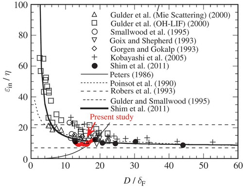
Figure 4b shows the streamwise development of inner cutoffs, , , and , computed using the 3D and 2D box-counting methods. The inner cutoffs in Figure 4b are normalized using the Kolmogorov length scale in unburned region where at each streamwise position. The inner cutoffs are . Peters (2000) showed that the inner cutoff is the Gibson scale for the corrugated flamelets regime and the Obukhov–Corrsin scale (or Kolmogorov length scale for the unity Schmidt number flame) for the thin reaction zones regime. It is also reported that the inner cutoff is scalable with the Kolmogorov length scale and the flame thickness (Chakraborty and Klein, 2008; Gülder and Smallwood, 1995), and also with the Gibson scale (Chakraborty and Klein, 2008). The present results show that and , where is the Gibson scale in the unburned region at each streamwise position. However, it cannot be concluded whether the inner cutoff is scalable with the Gibson scale. The correlating equation for the inner cutoff in Eq. (4) considers the dependency on the flame thickness as well as the Kolmogorov length scale. Unlike the fractal dimensions shown in Figure 4a, the effect of the large-scale roller structure resulted from KH instability is not clearly visible. In Figure 5, is plotted against , where is the most expected diameter of coherent fine scale eddies () (Tanahashi et al., 2001; Wang et al., 2007). Inner cutoffs and models reported in previous studies (Goix and Shepherd, 1993; Gorgen and Gökalp, 1993; Gülder and Smallwood, 1995; Gülder et al., 2000; Kobayashi et al., 2005; Peters, 1986; Poinsot et al., 1990; Roberts et al., 1993; Shim et al., 2011; Smallwood et al., 1995) are also shown in Figure 5. The 3D inner cutoffs obtained in the present DNS have a comparable trend with previous experimental and numerical results shown in the figure. Also, the model in Shim et al. (2011) employed in the present FDSGS combustion modelling approach mentioned in Eq. (4) shows an overall agreement with the measured and simulated results in a range of and turbulent flame configuration, when Kolmogorov length scale is precisely given.

Figure 4. Streamwise development of the (a) fractal dimension and (b) the inner cutoff of flame surfaces using 3D and 2D box-counting methods.

Figure 5. Dependence of the inner cutoff on . Lines: model values, and symbols: values from DNS and experiments.

Static tests of SGS combustion models

Procedure of the static test

The evaluation of the FDSGS combustion model is carried out by means of a priori tests first. Figure 6 shows the instantaneous temperature distribution and flame surfaces defined as contours of the turbulent plane jet flame simulated using the DNS. For LES analysis, the DNS temperature field is spatially filtered in a density-weighted manner using a Gaussian or top-hat filter kernel, although the choice of filter type does not influence the results as mentioned later. The filter width is set to be or in the static tests. The LES flame surfaces are defined as iso-surfaces in the filtered temperature field. Samples for the present evaluation are taken from the region along iso-surfaces with a thickness that can be scaled by LES mesh size . A similar sampling procedure to include all samples forming the flame fronts that could appear on LES meshes of size of was used in a previous study (Yoshikawa et al., 2013). The FDSGS combustion model, introduced in the section “Fractal Dynamic SGS Combustion Model,” is applied to the filtered DNS data to compute model values of fractal dimension, Kolmogorov length scale, and flame surface area, which are compared with the values obtained directly from the DNS results. In the static test, the Smagorinsky constant in the FDSGS combustion model is set to .

Figure 6. Temperature (in K) distribution on an instantaneous field obtained from the DNS of the turbulent jet premixed flame at . The flame surfaces represented by contour are also shown.

Predictions of fractal dimension and Kolmogorov length scale

Figure 7 shows the streamwise distributions of the fractal dimensions computed directly from the DNS using 3D box-counting and predicted from filtered field by using the procedure described in the section “Fractal Dynamic SGS Combustion Model.” The values of samples forming reaction zones described above are averaged over the – plane at each streamwise distance. To prevent unphysical values, the dimensions are constrained within a 2.0–3.0 range. Although the shown results are obtained using the Gaussian filter kernel with and , the top-hat filter is also tested (not shown) and the choice of filter type does not unduly change the result. For both filter sizes, the fractal dimensions predicted by the FDSGS combustion model increase with and show two peaks at and ; this trend is consistent with the DNS results. The modeled using CV of yields slightly closer values to the DNS values than that with the CV of , although this difference is still relatively small. These results demonstrate that the approach of computing fractal dimension to be used in the FDSGS combustion model predicts fractal dimensions adequately, which is independent of filter size, filter type, and control volume in the presence of strong mean shear with turbulence.

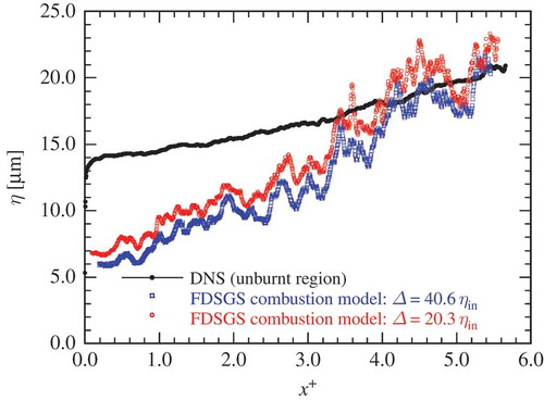
Figure 8 shows variations of Kolmogorov length scale computed from the Gaussian filtered DNS fields using Eq. (6) in the FDSGS combustion modelling approach. Top-hat filters are also tested, and the results do not change significantly. The values of Kolmogorov length scale of samples are averaged over the – plane, on par with Figure 7. The variation of Kolmogorov length scale in the region having directly computed from the DNS data in the same manner is also shown, whose value increases with and the FDSGS combustion model predicts the trend. In the region of , Kolmogorov length scale predicted by the model is smaller than that of the DNS data. This may be due to the assumption of the local equilibrium state at SGS, which is not well satisfied in the near field of the inlet. In the region of , the model predicts Kolmogorov length scale adequately being independent of filter type and filter width.

Figure 7. Streamwise development of the fractal dimensions of the flame surfaces obtained from the DNS data and predicted by the FDSGS combustion model with the Gaussian filters of (a) and (b) .

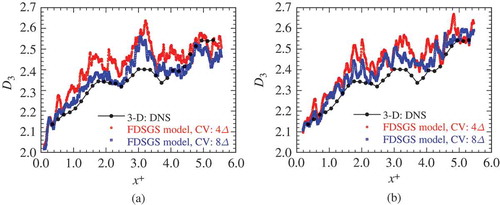
Figure 8. Streamwise distributions of Kolmogorov length scale obtained from the DNS data and computed using the FDSGS combustion model with the Gaussian filters.

Flame surface area predicted by the FDSGS combustion model

As described in the “Introduction,” a modeled value of flame surface area is required to close a reaction progress variable transport equation. This is computed based on the procedure described in the section “Fractal Dynamic SGS Combustion Model,” using the predicted fractal dimension and modeled Kolmogorov length scale, already tested in the previous subsection, “Predictions of Fractal Dimension and Kolmogorov Length Scale.” Since it is found that Kolmogorov length scale is modeled adequately when turbulence is developed well, which happens at in the present case, the test is performed for this region. In addition, a small number of samples having are chosen for flame surface area evaluation, since negative values are not physical, as shown in Eq. (6).

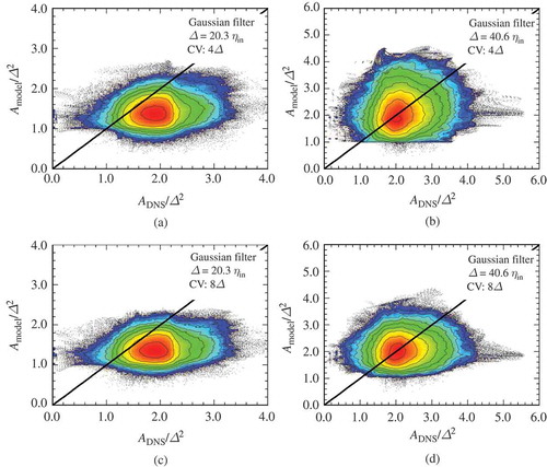
The joint probability density functions (JPDFs) of the flame surface areas obtained from the DNS data and predicted by the FDSGS combustion model for two different Gaussian filter sizes and CVs are shown in Figure 9. As shown in Figure 9, the most probable values of the flame surface areas modeled by the FDSGS combustion model are almost identical to those of the DNS data when being independent of the CV size. This independence is also true for filter type by comparing Gaussian and top-hat filters (not shown). For smaller filter size, , the most probable is slightly deviated from the DNS value, but they are still close. This less-accurate performance for smaller filter size would be attributed to the assumption of the scale separation in high Reynolds number turbulence: for a smaller filter width, the assumption in Eq. (5) cannot be satisfied sufficiently. The predicted values scatter partly because of the constant Smagorinsky coefficient. Using a dynamic Smagorinsky model is one way for improvement of the accuracy.

Figure 9. JPDFs of flame surface areas obtained from the DNS data and modeled using the FDSGS combustion model with the Gaussian filter of (a, c) and (b, d) . The CV is set to be (a, b) and (c, d) . The black diagonal line represents the perfect agreement with the DNS results. The spacing of contour lines is logarithmically spaced by a factor of two.

For a comparison, other SGS combustion models listed in Table 1 are also tested in the same a priori manner, and the results are shown in Figure 9. The SGS turbulent velocity fluctuations, , required for each model are calculated from the DNS data. The combustion models of Colin et al. (2000) and Charlette et al. (2002a) are proposed in the thickened flame context and the thickening factor, , is set to 1.0 to eliminate effects other than the flame surface area modeling for the present tests. Figure 10 shows JPDFs of the flame surface areas directly computed from the DNS results and predicted using the listed models with two different filter sizes. With the model reported in Charlette et al. (2002a), a term in a square root in the fitting function becomes negative and the model is not applicable for the present configuration. The flame surface areas predicted by the models reported in Colin et al. (2000) and Flohr and Pitsch (2000) are almost constant values and are considerably smaller than those of the DNS data. The underestimate by the model of Colin et al. (2000) may be due to the equilibrium assumption of the strain rate and curvature terms in the transport equation of the flame surface density. The results with the model of Flohr and Pitsch (2000) indicate that a simple model formulation based on several non-dimensional parameters is unsuccessful. The flame surface areas computed using Pitsch and Duchamp De Lageneste (2002) are closer to those of the DNS data, especially for the large filter size, than the values based on the other two models. However, the model slightly underestimates the area possibly because of the equilibrium assumption of the production and attenuation of SGS scalar variance.

Figure 10. JPDFs of flame surface areas obtained from the DNS data and computed using several SGS combustion models of Colin et al. (2000) (a, d), Flohr and Pitsch (2000) (b, e), and Pitsch and Duchamp De Lageneste (2002) (c, f) with the Gaussian filters of (top) and (bottom).

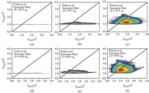
Table 1. Descriptions of conventional SGS combustion models compared in the present static tests.

	Expressions and parameters for the wrinkling factor
Colin et al. (2000)
	,
Flohr and Pitsch (2000)
Charlette et al. (2002a)
Pitsch and Duchamp De Lageneste (2002)
	,

Dynamic tests of SGS combustion models

Large eddy simulation of the turbulent jet premixed flame

Large eddy simulation of the turbulent combustion in the identical configuration and condition to the DNS is performed and discussed in this section for a posteriori testing of the FDSGS combustion model. The LES code solves the following conservation equations for mass:

(12)

and momentum:

(13)

and a transport equation of a reaction progress variable:

(14)

where the subscript (and appears later) denotes a quantity in the unburned (burned) mixture and is the SGS scalar flux, . Here, the reaction progress variable is based on temperature and defined as:

(15)

where and are the unburned and burned mixture temperatures of the corresponding one-dimensional unstrained laminar flame. Mass fractions of chemical species are binarized with values in the unburned and burned mixture composition in the laminar flame as:

(16)

Here, is a value of corresponding to the temperature, , and is 0.3175 in the present condition. The SGS stress tensor , which is modeled using the Smagorinsky model, and Smagorinsky constants of two different values, or , are used. The SGS turbulent scalar flux is modeled using a gradient diffusion model, where the turbulent Schmidt number, , is set to be or . The FDSGS combustion model and several models reported previously, summarized in Table 2, are used as SGS combustion models to obtain flame wrinkling factor to close Eq. (14). A Smagorinsky-type model (Flohr and Pitsch, 2000) is employed to estimate the SGS turbulent velocity fluctuation, , in the conventional models (Chatakonda et al., 2010; Colin et al., 2000; Fureby, 2005; Flohr and Pitsch, 2000):

(17)

Table 2. Conventional SGS combustion models considered in the present dynamic tests.

	Expressions and parameters for the wrinkling factor
Flohr and Pitsch (2000)
Colin et al. (2000)
	,
Fureby (2005)
Chatakonda et al. (2010)
	, ,

The convection term of the transport equation is spatially discretized using a fifth-order weighted essentially non-oscillatory (WENO) scheme (Jiang and Peng, 2000; Liu et al., 1994), while the other terms and equations are discretized using a fourth-order central finite difference scheme. Time integration is achieved by a third-order Runge–Kutta scheme.

For the inflow boundary, the same HIT field as the one used in the DNS is filtered with the Gaussian and cutoff filters, and superimposed on the mean inflow velocity in Eq. (11). Turbulence characteristics of the inflow turbulence are the same as the ones used in the DNS. The mesh sizes , the computational domain sizes , and the grid dimensions of the DNS and the LES are summarized in Table 3.

Table 3. Computational conditions of the LES and the DNS.

		mm
DNS	1.36	20 × 16 × 8	1281 × 1025 × 513
LES11	10.8	20 × 16 × 8	161 × 129 × 65
LES22	21.7	20 × 16 × 8	81 × 65 × 33
LES43	43.3	40 × 48 × 8	81 × 97 ×17

Evaluations of SGS combustion models

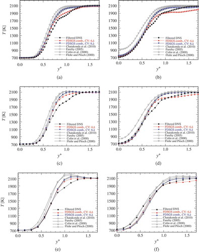
Figure 11 shows the instantaneous temperature iso-contour lines in the spanwise mid – plane for the LES using the FDSGS combustion model with CV of size and for the DNS data. The overall flame shapes at large scale from the LES show qualitatively good agreement with the DNS data. The mean temperature variations in the -direction at and for the LES with and and for the DNS data filtered with the Gaussian and cutoff filters are also shown in Figure 12. For comparison, LES results based on several SGS combustion models reported previously are also shown (Chatakonda et al., 2010; Colin et al., 2000; Fureby, 2005; Flohr and Pitsch, 2000). Although the LES with these models can reproduce the temperature trend very well, the results based on the model of Flohr and Pitsch (2000) deviate from the DNS values in the downstream region. As explained in the last paragraph in this section, this could be relevant of the use of the Smagorinsky-type model [Eq. (17)] for the SGS turbulent velocity fluctuation. The variations simulated with the present FDSGS combustion model are closer to the filtered DNS results overall, regardless of the size of CV, filter size and streamwise position under the present simulation conditions.

Figure 11. Instantaneous progress variable contours () in the spanwise mid-plane for DNS (gray line), LES11 (thin line), LES22 (dashed line), and LES43 (dashed-dotted line) with the FDSGS combustion model and CV size of at (a) and (b) .

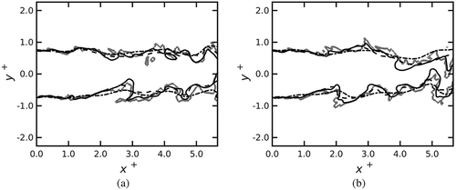
Figure 12. Mean temperature distributions in -direction for the filtered DNS data and results of LES11 (a, b), LES22 (c, d), and LES43 (e, f) at (a, c, e) and (b, d, f) in the case of and .

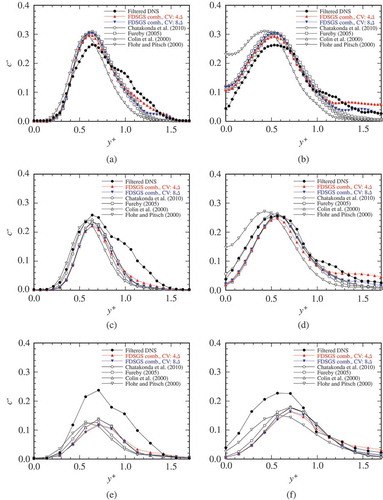
Figure 13 shows the transverse distributions of root-mean-square (RMS) values of the filtered progress variable fluctuation from its spanwise average, , for the filtered DNS data and the LES results. Comparing with the temperature plots in Figure 12, the deviations of from the filtered DNS variation are large for all the models shown. However, the present FDSGS combustion model and the models reported in Colin et al. (2000), Fureby (2005), and Chatakonda et al. (2010) show reasonable performance regardless of filter size and streamwise locations. The LES with the FDSGS combustion model also predicts peak positions of the transverse distributions for . From Figures 12 and 13, the FDSGS combustion model and the models of Colin et al. (2000), Fureby (2005), and Chatakonda et al. (2010) are considered to be applicable to premixed flames in turbulent shear flow. The model of Flohr and Pitsch (2000) may give better predictions for lower Damköhler number flames as discussed in their work. As discussed in the previous paragraph, the results based on the model of Flohr and Pitsch (2000) show relatively large deviations from the DNS values. This could be due to the Smagorinsky-type model for , which is discussed in the next paragraph. As shown in Figure 13, the two results with CVs of and are almost identical, except at the downstream co-flow region where the turbulence is relatively weak.

Figure 13. Variations of in -direction for the filtered DNS data and results of LES11 (a, b), LES22 (c, d), and LES43 (e, f) at (a, c, e) and (b, d, f) in the case of and .

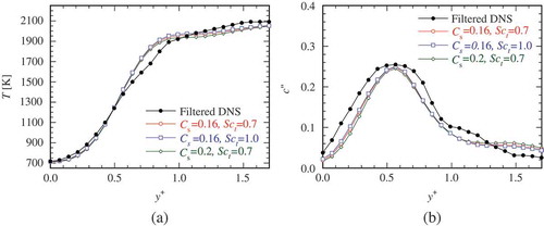
Effects of the model constants on the LES results are also studied by comparing the LES with different Smagorinsky constants and turbulent Schmidt numbers. Figure 14 shows the transverse distributions of the mean temperature and at for LES22 with the FDSGS combustion model. These plots show the insensitivity of the LES results to the choice of the Smagorinsky constant and the turbulent Schmidt number under the conditions considered in the present study when the FDSGS combustion model is employed. Similar trends are observed also for the LES with the other conventional SGS combustion models.

Figure 14. Transverse distributions of mean temperature (a) and RMS values of progress variable fluctuation (b) at for the filtered DNS data and LES22 simulated using the FDSGS combustion model. The size of CV is and different Smagorinsky constants and turbulent Schmidt numbers as labeled are used.

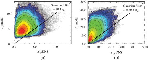
Finally, the performance comparison of the model by Flohr and Pitsch (2000) in the static (the section “Flame Surface Area Predicted by the FDSGS Combustion Model”) and the dynamic (the section “Evaluations of SGS Combustion Models”) tests shows that the model’s over-prediction of the turbulent flame speed (flame surface area) is observed in the dynamic tests as shown in Figure 12, but not in the static tests. As explained in the section “Large Eddy Simulation of the Turbulent Jet Premixed Flame,” the Smagorinsky-type model [Eq. (17)] is employed to model in the dynamic tests while the quantity is directly obtained for the static tests. This suggests that the Smagorinsky-type model is oversimplified for the present turbulent combustion configuration. To investigate this, computed by using the Smagorinsky-type model [Eq. (17)] and one directly obtained from the DNS results are compared in the manner of the static tests. Figure 15 shows JPDFs of predicted using the model and obtained from the DNS for for a turbulent planar premixed flame (Yoshikawa et al., 2013) and the present jet flame. The model over-predicts in general. Since an over-predicted increases the modeled flame surface area, the over-predicted shown in Figure 15 is possibly one of the reasons that the LES with the model of Flohr and Pitsch (2000) tends to show higher temperature than the DNS data in the present LES. For further model development, the FDSGS combustion model has an additional advantage in simplicity that the model does not require .

Figure 15. JPDFs of the SGS turbulent velocity fluctuations predicted by the Smagorinsky-type model (Flohr and Pitsch, 2000) and obtained from the DNS data for . Results for (a) turbulent planar premixed flame and (b) the present jet flame. Typical Smagorinsky constants are used: for the planar case and for the jet case.

Conclusions

In the present study, a fractal analysis on flame surfaces and static tests using DNS data of a hydrogen-air turbulent jet premixed flame were performed to investigate fractal characteristics and evaluate the fractal dynamic SGS combustion model for turbulent premixed flames with strong mean shear.

The fractal analysis shows that the fractal dimension of the flame surfaces of the turbulent jet premixed flame increases with the downstream distance from the inlet, and the fractal dimension calculated with the 3D box-counting method reaches about 2.54 in the region where turbulence is fully developed by mean shear. At the positions where large-scale coherent structures roll up and pair, the fractal dimension shows peaks. The DNS analysis shows that a model employed in the present approach for inner cutoff (Shim et al., 2011) could be used in LES of complicated combustion problems.

From the static tests of SGS combustion models, it was revealed that the procedure applied in the FDSGS combustion model adequately predicts the fractal dimensions of the flame surfaces, Kolmogorov length scale, and flame surface area. Although the fractal dimensions calculated with control volume of size are slightly larger than those obtained from the DNS data, the choice of control volume size does not influence the overall performance of the model. The flame surface area predicted by the FDSGS combustion model shows better correlations with the DNS results when a larger LES filter width is considered, although the performance is consistently reasonable for the range of filter sizes tested.

Dynamic model evaluations are also carried out by conducting a series of LES using the FDSGS and other combustion models. In the dynamic tests, the mean temperature distributions obtained from the LES with the FDSGS combustion model show good agreement with the filtered DNS fields. The LES with the FDSGS combustion model also predicts peak positions of transverse distributions for the RMS values of progress variable fluctuation. The static and dynamic tests also revealed that one of the strengths in the FDSGS combustion modeling approach is that the model does not require SGS turbulent velocity fluctuation, since modeling of this quantity is straightforward for neither homogeneous turbulence nor turbulent shear flows.

Finally, the overall flame propagation characteristics would be sensitive to the SGS scalar flux term in Eq. (14). The choice of the SGS stress model also affects the LES results. The development and assessment for scalar flux and stress models will be performed in future work.

Funding

K. H., Y. M., M. S., Y. N., and M. T. acknowledge the support of the Council for Science, Technology and Innovation (CSTI), Cross-ministerial Strategic Innovation Promotion Program (SIP), “Innovative Combustion Technology” (Funding agency: JST).

Additional information

Funding

K. H., Y. M., M. S., Y. N., and M. T. acknowledge the support of the Council for Science, Technology and Innovation (CSTI), Cross-ministerial Strategic Innovation Promotion Program (SIP), “Innovative Combustion Technology” (Funding agency: JST).

References

- Baum, M., Poinsot, T., and Thevenin, D. 1994. Accurate boundary conditions for multicomponent reactive flows. J. Comput. Phys., 106, 247–261.
- Brown, P.N., Byrne, G.D., and Hindmarsh, A.C. 1989. VODE: A variable-coefficient ODE solver. SIAM J. Sci. Statist. Comput., 10, 1038–1051.
- Chakraborty, N., and Klein, M. 2008. A priori direct numerical simulation assessment of algebraic flame surface density models for turbulent premixed flames in the context of large eddy simulation. Phys. Fluids, 20, 085108.
- Charlette, F., Meneveau, C., and Veynante, D. 2002a. A power-law flame wrinkling model for LES of premixed turbulent combustion Part I: Non-dynamic formulation and initial tests. Combust. Flame, 131, 159–180.
- Charlette, F., Meneveau, C., and Veynante, D. 2002b. A power-law flame wrinkling model for LES of premixed turbulent combustion Part II: Dynamic formulation. Combust. Flame, 131, 181–197.
- Chatakonda, O., Hawkes, E. R., Aspden, A. J., Kerstein, A. R., Kolla, H., and Chen, J. H. 2013. On the fractal characteristics of low Damk¨ohler number flames. Combust. Flame, 160, 2422–2433.
- Chatakonda, O., Hawkes, E. R., Brear, M. J., Chen, J. H., Knudsen, E., and Pitsch, H. 2010. Modeling of the wrinkling of premixed turbulent flames in the thin reaction zones regime for large eddy simulation. In Proceedings of the Center for Turbulence Research Summer Program, P. Moin, J. Larsson, and N. Mansour (Eds.), Stanford University, pp. 271–280.
- Cintosun, E., Smallwood, G. J., and Gülder, Ö. L. 2007. Flame surface fractal characteristics in premixed turbulent combustion at high turbulence intensities. AIAA J., 45, 2785–2789.
- Cohé, C., Halter, F., Chauveau, C., Gökalp, I., and Gülder, Ö. L. 2007. Fractal characterisation of high-pressure and hydrogen-enriched CH4-air turbulent premixed flames. Proc. Combust. Inst., 31, 1345–1352.
- Colin, O., Ducros, F., Veynante, D., and Poinsot, T. 2000. A thickened flame model for large eddy simulation of turbulent premixed combustion. Phys. Fluids, 12, 1843–1863.
- Damköhler, G. 1940. Der einfluss der turbulenz auf die flammengeschwindigkeit in gasgemischen. Z. Elektrochem., 46(11), 601–626.
- Flohr, P., and Pitsch, H. 2000. A turbulent flame speed closure model for LES of industrial burner flows. In Proceedings of the Center for Turbulence Research Summer Program, P. Moin, W.C. Reynolds, and N. Mansour (Eds.), Stanford University, pp. 169–179.
- Fureby, C. 2005. A fractal flame-wrinkling large eddy simulation model for premixed turbulent combustion. Proc. Combust. Inst., 30, 593–601.
- Gicquel, L. Y. M., Staffelbach, G. and Poinsot, T. 2012. Large eddy simulation of gaseous flames in gas turbine combustion chambers. Prog. Energy Combust. Sci., 38, 782–817.
- Goix, P. J., and Shepherd, I. G. 1993. Lewis number effects on turbulent premixed flame structure. Combust. Sci. Technol., 91, 191–206.
- Gorgen, A. Ü. A., and Gökalp, S. 1993. A planar laser induced fluorescence study of turbulent flame kernel growth and fractal characteristics. Combust. Sci. Technol., 92, 265–290.
- Gouldin, F. C. 1987. An application of fractals to modeling premixed turbulent flames. Combust. Flame, 68, 249–266.
- Gülder, Ö. L. 1990. Turbulent premixed combustion modelling using fractal geometry. Proc. Combust. Inst., 23, 835–842.
- Gülder, Ö. L., and Smallwood, G. J. 1995. Inner cutoff scale of flame surface wrinkling in turbulent premixed flames. Combust. Flame, 103, 107–114.
- Gülder, Ö. L., Smallwood, G. J., Wong, R., Snelling, D. R., Smith, R., Deschamps, B. M., and Sautet, G. C. 2000. Flame front surface characteristics in turbulent premixed propane/air combustion. Combust. Flame, 120, 407–416.
- Gutheil, E., Balakrishnan, G., and Williams, F. A. 1993. Structure and extinction of hydrogen–air diffusion flames. In Lecture Notes in Physics: Reduced Kinetic Mechanisms for Applications in Combustion Systems, N. Peters and B. Rogg (eds.), Springer, New York, pp. 177–195.
- Haworth, D. C. 2010. Progress in probability density function methods for turbulent reacting flows. Prog. Energy Combust. Sci., 36, 168–259.
- Jiang, G.-S., and Peng, D. 2000. Weighted ENO schemes for Hamilton-Jacobi equations. SIAM J. Sci. Comput., 21, 2126–2143.
- Kerstein, A. R. 1988. Fractal dimension of turbulent premixed flames. Combust. Sci. Technol., 60, 441–445.
- Kim, J., and Pope, S. B. 2014. Effects of combined dimension reduction and tabulation on the simulations of a turbulent premixed flame using a large-eddy simulation/probability density function method. Combust. Theor. Model., 18(3), 388–413.
- Knikker, R., Veynante, D., and Meneveau, C. 2004. A dynamic flame surface density model for large eddy simulation of turbulent premixed combustion. Phys. Fluids, 16(11), L91–L94.
- Kobayashi, H., and Kawazoe, H. 2000. Flame instability effects on the smallest wrinkling scale and burning velocity of high-pressure turbulent premixed flames. Proc. Combust. Inst., 28, 375–382.
- Kobayashi, H., Seyama, K., Hagiwara, H., and Ogami, Y. 2005. Burning velocity correlation of methane/air turbulent premixed flames at high pressure and high temperature. Proc. Combust. Inst., 30, 827–834.
- Lele, S. K. 1992. Compact finite difference schemes with spectral-like resolution. J. Comput. Phys., 103, 16–42.
- Liu, X.-D., Osher, S., and Chan, T. 1994. Weighted essentially non-oscillatory schemes. J. Comput. Phys., 115, 200–212.
- Mantzaras, J. 1992. Geometrical properties of turbulent premixed flames: Comparison between computed and measured quantities. Combust. Sci. Technol., 86, 135–162.
- Michalke, A. 1964. On the inviscid instability of the hyperbolic-tangent velocity profile. J. Fluid Mech., 19, 543–556.
- Minamoto, Y., Fukushima, N., Tanahashi, M., Miyauchi, T., Dunstan, T. D., and Swaminathan, N. 2011. Effect of flow-geometry on turbulence-scalar interaction in premixed flames. Phys. Fluids, 23(12), 125107.
- Miyauchi, T., Tanahashi, M., and Gao, F. 1994. Fractal characteristics of turbulent diffusion flames. Combust. Sci. Technol., 96, 135–154.
- Peters, N. 1986. Laminar flamelet concepts in turbulent combustion. Proc. Combust. Inst., 21, 1231–1250.
- Peters, N. 2000. Turbulent Combustion, Cambridge University Press, Cambridge, UK.
- Pitsch, H. 2002. A G-equation formulation for large-eddy simulation of premixed turbulent combustion. In Center for Turbulence Research Annual Research Briefs 2002, P. Moin, N. Mansour, and P. Bradshaw (Eds.), Stanford University, pp. 3–14.
- Pitsch, H. 2006. Large eddy simulation of turbulent combustion. Annu. Rev. Fluid Mech., 38, 453–482.
- Pitsch, H., and Duchamp De Lageneste, L. 2002. Large-eddy simulation of premixed turbulent combustion using a level-set approach. Proc. Combust. Inst., 29, 2009–2015.
- Poinsot, T., Veynante, D., and Candel, S. 1990. Diagrams of premixed turbulent combustion based on direct simulation. Proc. Combust. Inst., 23, 613–619.
- Poinsot, T. J., and Lele, S. K. 1992. Boundary conditions for direct simulations of compressible viscous flows. J. Comput. Phys., 101, 104–129.
- Roberts, W. L., Driscoll, J. F., Drake, M. C., and Goss, L. P. 1993. Images of the quenching of a flame by a vortex—to quantify regimes of turbulent combustion. Combust. Flame, 94, 58–69.
- Shim, Y., Tanaka, S., Tanahashi, M., and Miyauchi, T. 2011. Local structure and fractal characteristics of H2-air turbulent premixed flame. Proc. Combust. Inst., 33, 1455–1462.
- Shimura, M., Yamawaki, K., Fukushima, N., Shim, Y. S., Nada, Y., Tanahashi, M., and Miyauchi, T. 2012. Flame and eddy structures in hydrogen-air turbulent jet premixed flame. J. Turbul., 13, 1–17. DOI: 10.1080/14685248.2012.720022.
- Smallwood, G. J., Gülder, Ö. L., Snelling, D. R., Deschamps, B. M., and Gökalp, I. 1995. Characterization of flame front surfaces in turbulent premixed methane/air combustion. Combust. Flame, 101, 461–470.
- Tanahashi, M., Iwase, S., and Miyauchi, T. 2001. Appearance and alignment with strain rate of coherent fine scale eddies in turbulent mixing layer. J. Turbul., 2, 1–18. DOI:10.1088/1468-5248/2/1/006.
- Tanahashi, M., Wang, Y., Fujisawa, T., Sato, M., Chinda, K., and Miyauchi, T. 2007. Fractal geometry and mixing transition in turbulent mixing layer. In Proceedings of the Fifth International Symposium on Turbulence and Shear Flow Phenomena, R. Friedrich, N.A. Adams, J.K. Eaton, J.A.C. Humphrey, N. Kasagi, and M.A. Leschziner (Eds.), Munich, Germany, pp. 1187–1192.
- Thornber, B., Bilger, R. W., Masri, A. R., and Hawkes, E. R. 2011. An algorithm for LES of premixed compressible flows using the conditional moment closure model. J. Comput. Phys., 230, 7687–7705.
- Veynante, D., and Vervisch, L. 2002. Turbulent combustion modeling. Prog. Energy Combust. Sci., 28, 193–266.
- Wang, Y., Tanahashi, M., and Miyauchi, T. 2007. Coherent fine scale eddies in turbulence transition of spatially-developing mixing layer. Int. J. Heat Fluid Flow, 28, 1280–1290.
- Yoshikawa, I., Shim, Y. S., Nada, Y., Tanahashi, M., and Miyauchi, T. 2013. A dynamic SGS combustion model based on fractal characteristics of turbulent premixed flames. Proc. Combust. Inst., 34, 1373–1381.