A Priori Assessment of Scalar Dissipation Rate Closure for Large Eddy Simulations of Turbulent Premixed Combustion Using a Detailed Chemistry Direct Numerical Simulation Database

ABSTRACT

Algebraic and transport equation-based closures of Favre-filtered scalar dissipation rate (SDR) of the reaction progress variable, in the context of large eddy simulations, have been assessed using detailed chemistry direct numerical simulation (DNS) data of a stoichiometric H₂-air turbulent V flame. The Favre-filtered SDR and the unclosed terms of its transport equation have been extracted by explicitly filtering the DNS data for different choices of the reaction progress variable. An algebraic closure of SDR, which was proposed previously using simple chemistry DNS data, has been found to predict the Favre-filtered SDR satisfactorily for detailed chemistry DNS data for different choices of the reaction progress variable. Similarly, the models of the unclosed sub-grid convection, density variation, scalar-turbulence interaction, reaction rate gradient, molecular dissipation, and diffusivity gradient terms of the Favre-filtered SDR transport equation, which have previously been proposed based on simple chemistry DNS data, have been found to satisfactorily predict both the qualitative and quantitative behaviors of these unclosed terms for a range of filter widths , for two different choices of reaction progress variable in the case of the detailed chemistry DNS dataset considered in this analysis.

KEYWORDS:

• Direct numerical simulation
• Large eddy simulations
• Reaction progress variable
• Scalar dissipation rate
• Turbulent premixed combustion

Introduction

The rate of micro-mixing plays a key role in the fundamental physical understanding and modeling of turbulent reacting flows (Bilger, 2004). The quantity that characterizes the rate of micro-mixing is the scalar dissipation rate (SDR), which is often used for the probability density function (PDF) (Dopazo, 1994; O’Brien, 1980) and conditional moment closure (CMC) (Bilger, 2004; Klimenko and Bilger, 1999) methodologies especially in the context of non-premixed combustion modeling. Bray (1980) demonstrated that the Favre-averaged SDR in the context of Reynolds averaged Navier Stokes (RANS) plays a key role in the closure of mean reaction rate for infinitely fast chemistry (i.e., for large values of Damköhler number). It was subsequently demonstrated by Chakraborty and Cant (2011) using scaling arguments and direct numerical simulation (DNS) data that the SDR-based reaction rate closure derived by Bray (1980) also remains valid for low Damköhler number combustion as long as the flamelet assumption remains valid. A number of recent analyses (Butz et al., 2015; Dunstan et al., 2013; Gao et al., 2014a, 2014b; Langella et al., 2015; Ma et al., 2014a) demonstrated that the SDR-based closure for RANS proposed by Bray (1980) can also be used for large eddy simulations (LES) when the filter size is much greater than the thermal flame thickness , where , and are the adiabatic flame, unburned gas, and instantaneous temperatures, respectively. The SDR-based filtered reaction rate closure of reaction progress variable for large filter widths (i.e., ) takes the following form (Butz et al., 2015; Dunstan et al., 2013; Gao et al., 2014a, 2014b; Ma et al., 2014a):

(1)

where is the density, is the instantaneous SDR, is the Favre-filtered value of a quantity with the over-bar indicating an LES filtering operation, and D is the diffusivity of reaction progress variable . In Eq. (1), is the reacting mode probability density function (pdf) of c and the subscript ‘L’ refers to the planar laminar flame conditions. The numerical value of remains within a range of 0.7–0.9 for typical hydrocarbon-air mixtures when is chosen to be a smooth function, regardless of its exact form (Bray, 1980). There are other alternative approaches of LES premixed combustion modeling, such as the level-set (Freitag, 2007; Peters, 2000; Pitsch and Duchamp-de-Lageneste, 2002), flame surface density (FSD) (Chakraborty and Cant, 2009a; Chakraborty and Klein, 2008; Hawkes and Cant, 2000, 2001; Hernandez-Perez et al., 2011; Ma et al., 2013, 2014b; Reddy and Abraham, 2012), and the artificially thickened flame (ATF) (Charlette et al., 2002a, 2002b; Kuenne et al., 2011; Veynante and Poinsot, 1997) methods, which also depend on flamelet assumption similar to the SDR-based reaction rate closure. There are other approaches [e.g., Eulerian stochastic field method (Jones et al., 2012)], which could be used for both flamelet and non-flamelet-type combustion but at the expense of higher computational cost than the SDR, level-set, and ATF approaches. The inter-relation between the temperature field and the flame surface is not straightforward and often empirically formulated in the level-set approach, whereas the temperature and species fields are inherently linked by combustion thermo-chemistry in the FSD, SDR, and ATF methodologies. Most wrinkling factor models used in the ATF methodology were proposed for unity Lewis number combustion but they do not adequately perform for non-unity Lewis number flames (Katragadda et al., 2012). It has been found that (Chakraborty and Cant, 2011; Gao et al., 2014a) that the SDR-based reaction rate closure remains valid for a range of different Lewis numbers , whereas the reaction rate closure by FSD needs a correction factor, which is a function of Lewis number (Chakraborty and Cant, 2011). This makes the SDR-based closure a promising computationally inexpensive methodology for reaction rate closure in turbulent premixed combustion.

A number of analyses concentrated on SDR closures for premixed turbulent combustion in the context of RANS (Ahmed and Swaminathan, 2013; Chakraborty et al., 2008a; 2010, 2011; Chakraborty and Swaminathan, 2010, 2011, 2013; Dong et al., 2013; Kolla et al., 2009; Kolla and Swaminathan, 2010a, 2010b; Mantel and Borghi, 1994; Mura and Borghi, 2003; Mura et al., 2008, 2009; Sadasivuni et al., 2012) but limited effort has been directed to the closure of SDR for LES (Butz et al., 2015; Dunstan et al., 2013; Gao et al., 2014a, 2014b, 2015a, 2015b; Gao and Chakraborty, 2016; Langella et al., 2015; Ma et al., 2014a). Recently, Gao et al. (2014a, 2014b, 2015a) proposed algebraic closures of for both static and dynamic model coefficients and assessed their validity by extracting the relevant quantities from explicitly filtered DNS data (i.e., a priori assessment). These closures have subsequently been implemented in actual LES simulations for a number of configurations (Butz et al., 2015; Langella et al., 2015; Ma et al., 2014a) for the purpose of model validation (i.e., a-posteriori analysis), and a satisfactory level of agreement has been obtained with experimental measurements. However, all of the aforementioned analyses have been carried out in the context of simple single-step chemistry and thus it is important to compare the statistical behaviors of the SDR and its transport obtained from simple chemistry DNS data with corresponding statistics extracted from detailed chemistry DNS, to ascertain whether the modeling assumptions used for simple chemistry remain valid for predicting the dissipation rates of major species (i.e., SDRs of major reactants and products) in the context of detailed chemistry and transport. Moreover, it is possible to define based on different species mass fractions in the context of detailed chemistry, and thus it is important to analyze if the choice of affects the statistics of SDR transport. Furthermore, most existing SDR closures have been proposed for unity Lewis number flames, but is known to have significant influences on the statistical behavior of the unclosed terms of the Favre-averaged SDR transport equation in the context of RANS (Chakraborty and Swaminathan, 2010). Similar qualitative behavior has been observed for LES (Gao et al., 2014b; Gao and Chakraborty, 2016), and the sub-models proposed by Gao et al. (2015b) for the unclosed terms of transport equations for the thermo-diffusively neutral flames needed modification to account for the non-unity Lewis number effects. Different chemical species have different Lewis numbers; thus, it remains to be assessed if the models for the SDR transport equation, which were previously proposed based on simple chemistry DNS data, are also valid in the context of detailed chemistry DNS data. In this respect the main objectives of the current analysis are:

1. To indicate the influences of the definition of reaction progress variable on the SDR statistics.

2. To assess if the closures of SDR and its transport, which were proposed previously based on simple chemistry DNS data, remain valid for a detailed chemistry DNS data.

In order to meet these objectives, the Favre-filtered SDR statistics obtained from a DNS dataset of a turbulent stoichiometric -air V-shaped oblique premixed flame (Minamoto et al., 2011) has been considered.

The rest of the article is organized as follows. The information related to mathematical background and numerical implementation is provided in the next two sections. This is followed by the presentation of results and its subsequent discussion. Finally, the main findings are summarized and conclusions are drawn.

Mathematical background

For single step chemistry can be uniquely defined but in the context of detailed chemistry one can obtain different distributions of depending on its definition. For the detailed chemistry turbulent H₂-air V-flame dataset, two alternative definitions of reaction progress variable have been considered based on H₂ and H₂O mass fractions in the following manner:

(1)

where the subscripts 0 and indicate the values in unburned reactants and fully burned products, respectively. Thus, one gets , , , and for stoichiometric H₂-air premixed flame. Equation (1) is valid not only for stoichiometric flames but for all equivalence ratios provided correct values of , , , and corresponding to the equivalence ratio in question are used. The reaction progress variable is required to increase monotonically from 0 in unburned reactants to 1.0 in fully burned products and that is why the reaction progress variable in Eq. (1) is defined based on the mass fraction of either a major reactant or a major product species, which is consistent with several previous analyses (Chakraborty et al., 2008b; Hawkes and Chen, 2005, 2006; Kolla et al., 2009; Kolla and Swaminathan, 2010a, 2010b; Rogerson and Swaminathan, 2007). It is worth noting that it will be improper to use the mass fraction of an intermediate species in Eq. (1), because in this particular case the reaction progress variable does not monotonically increase from 0 to 1 from the unburned to burned gases. Equation (1) reduces to when the value of is equal to zero, which is only true when either a fuel-lean or a stoichiometric flame is considered. Similarly, becomes when the product species is absent in the unburned gas [i.e., ]. The non-dimensional temperature is often used as the reaction progress variable but instantaneous dimensional temperature may assume super-adiabatic values (i.e., ) even under a globally adiabatic condition in the presence of significant differential diffusion of heat and species. This yields an unphysical value of reaction progress variable, which is greater than unity. In this respect, Eq. (1) is valid for all values of global Lewis number and equivalence ratio. However, most combustion models have been proposed for thermo-diffusively neutral conditions so it might be advantageous to define the reaction progress variable based on a major reactant/product species, which has a Lewis number close to unity. In this respect, is likely to be more advantageous than .

Recently, Gao et al. (2014a) proposed an algebraic closure for the Favre-filtered SDR in the following manner:

(2)

where is the unstrained laminar burning velocity, is the thermal flame thickness, is the heat release parameter, is the Lewis number of the species based on which the reaction progress variable is defined, and is a bridging function, with being the LES filter width. In Eq. (2), , and are the model parameters and Gao et al. (2014a) suggested the following expressions of these parameters:

; (3)

where and are the local sub-grid Damköhler and Karlovitz numbers, respectively, with being the sub-grid level velocity fluctuation. Moreover, is a thermo-chemical parameter, which is expressed as (Kolla et al., 2009; Rogerson and Swaminathan, 2007):

(4)

Interested readers are referred to Gao et al. (2014a, 2014b, 2015a), Ma et al. (2014a), and Butz et al. (2015) for the theoretical justification of the model expression given by Eq. (2). It was shown in previous analyses (Gao et al., 2014a, 2014b; Ma et al., 2014a) that Eq. (2) satisfactorily captures both volume-averaged and local behaviors of Favre-filtered SDR for different values of and based on simple chemistry DNS data in the conventional canonical configuration. The performance of the model given by Eq. (2) for a detailed chemistry DNS data for turbulent H₂-air V-shaped premixed flame will be assessed in the Results and Discussion section for Favre-filtered SDRs of reaction progress variables based on H₂ and H₂O mass fractions (i.e., and ).

The transport equation of Favre-filtered SDR takes the following form (Gao et al., 2014a, 2014b, 2015b; Gao and Chakraborty, 2016):

(5)

where is the ith component of velocity vector. On the left-hand side of Eq. (5) the terms denote the transient effects and resolved advection of , respectively. The term depicts the molecular diffusion of , and the terms , and are expressed as:

(6a)

(6b)

(6c)

(6d)

(6e)

(6f)

The term denotes sub-grid convection, whereas denotes the effects of density variation due to heat release. The term is governed by the alignment of with local strain rate , and this term is commonly referred to as the scalar-turbulence interaction term. The term arises due to the correlation between and , whereas denotes the molecular dissipation of SDR and these terms will henceforth be referred to as the reaction rate gradient term and dissipation term, respectively. The term represents the effects of variation. The terms , and are unclosed and need modeling. Furthermore, the modeling of depends on the modeling of sub-grid SDR flux . Gao et al. (2014b, 2015b) recently analyzed the statistical behaviors of these unclosed terms (i.e., and ) and proposed scaling estimates of these terms. These scaling estimates are summarized in Table 1 and these relations have subsequently been utilized to propose closures for , , and in the context of LES by Gao et al. (2015b) based on the assessment of model performance with respect to the corresponding quantities extracted from explicitly filtered simple chemistry DNS data of turbulent premixed flames with . These models have subsequently been modified to account for non-unity Lewis number effects by Gao and Chakraborty (2016). The models of , , and , as proposed by Gao and Chakraborty (2016), are summarized in Table 2. In Tables 1 and 2, , , , , and are the resolved components of , and , which are given by:

(7a)

(7b)

(7c)

(7d)

(7e)

Table 1. Summary of the scaling estimates of the relevant quantities according to Gao et al. (2014b).

Quantities	Scaling estimates
	where is an alternative flame thickness.
	where and .
	alternatively ; the above expressions can be combined as .
	where .
	where is the reference velocity scale for the mean flow.
	(T3S1) alternatively (T3S2) where is the sub-grid Karlovitz number.
	.
	where increases with decreasing .
	where increases with decreasing .
	alternatively where increases with decreasing .
	.
	.
	.

Table 2. Summary of the models for the unclosed terms of the SDR transport equation as proposed by Gao and Chakraborty (2016).

Term	Model expressions
	Model expression (FLUXG): where and .
	Model expression (T2G):where is the sub-grid Karlovitz number and .
	Model expression (T3G): where , , , , , and is the density-weighted sub-grid Damköhler number.
	Model expression (T4D2FG):where , , , , and .

The performance of the models listed in Table 2 will be assessed in the Results and Discussion section for detailed chemistry DNS data of a stoichiometric turbulent H₂-air V-shaped premixed flame for reaction progress variables based on H₂ and H₂O mass fractions (i.e., and ).

Numerical implementation

In the present study, a three-dimensional (3D) detailed H₂-air chemistry DNS data of a turbulent stoichiometric V-flame (Minamoto et al., 2011) has been considered. The V-flame case considers a stoichiometric premixed H₂-air mixture supplied at a temperature of 700 K and pressure 0.1 MPa with a mean inlet velocity (i.e., ). A detailed chemical kinetic mechanism involving 12 species and 27 reactions (Gutheil et al., 1993) has been used for the V-flame simulation and the temperature dependence of thermo-physical properties are considered according to the CHEMKIN database (Kee et al., 1986, 1989).

For V-flame simulation a rod of diameter is placed at a distance of 5 mm from the inlet boundary for the purpose of flame stabilization. The temperature, velocity, and species mass fraction within the rod is taken to be 2000 K, 0, and (where the subscript refers to the fully burned gas value of the species ). A Gaussian function of the following form has been used to smoothly blend the values at the rod with the corresponding freestream values (Minamoto et al., 2011):

(8)

where is a general primitive variable, is the radial co-ordinate from the center of the flame holder, and is the radius of the flame holder. The fluid velocity at the inlet boundary is specified as the summation of mean inlet velocity and velocity fluctuations. The velocity fluctuations at the inlet are obtained by scanning a plane through a frozen field of incompressible turbulent velocity field. The simulation domain is taken to be a rectangle of (), which is discretized using a uniform Cartesian grid of . This grid ensures about 20 points within and sufficient resolution of the boundary layer formed over the flame holder. It has been found that the values of and remain about 4 and 7, where , , and , respectively, with , and being the grid spacing in , and directions, respectively. Fourth-order finite-difference and third-order Runge–Kutta methods are used for spatial differentiation and explicit time-advancement, respectively. Turbulent inflow and non-reflecting outflow boundaries are specified in the stream-wise (i.e., x₁-direction) directions whereas the transverse () and span-wise () boundaries are considered to be non-reflecting outflow and periodic, respectively. All of the non-periodic boundaries are specified using the Navier Stokes characteristics boundary conditions (NSBC) technique (Poinsot and Lele, 1992). The inlet values of normalized mean inlet velocity, normalized rms turbulent velocity fluctuation, integral length scale to thermal flame thickness ratio , turbulent Reynolds number , Damköhler number , and Karlovitz number are summarized in Table 3 along with the value of heat release parameter , where and are the unburned gas density and viscosity, respectively. The thermo-chemical parameter is taken to be 0.78 following previous analysis (Minamoto et al., 2011). The flamelet assumption remains valid for the simulation parameters considered in this analysis (Peters, 2000). The simulation has been continued for 3 through-pass time (i.e., ), which corresponds to 8.91 chemical time scale (i.e., ).

Table 3. List of the non-dimensional parameters at the inlet for the V flame case, which are shown with a subscript ‘i’.

10.0	2.2	1.6	1.86	200	0.73	1.30

The Favre-filtered SDR and the unclosed terms of its transport equation of have been evaluated by explicitly filtering DNS data using a standard 3D Gaussian filter: (Boger et al., 1998; Charlette et al., 2002a, 2002b; Dunstan et al., 2013; Gao et al., 2014a, 2014b, 2015a, 2015b) and the filtered values of a general quantity is given by the following integral: . For this analysis, results will be presented for ranging from to . This range of filter widths is comparable to the range of used in several previous analyses (Boger et al., 1998; Charlette et al., 2002a, 2002b; Dunstan et al., 2013; Gao and Chakraborty, 2016; Gao et al., 2014a, 2014b, 2015a, 2015b), and cover a range of different length scales from comparable to up to , where is comparable to the integral length scale .

Results and discussion

Flame turbulence interaction

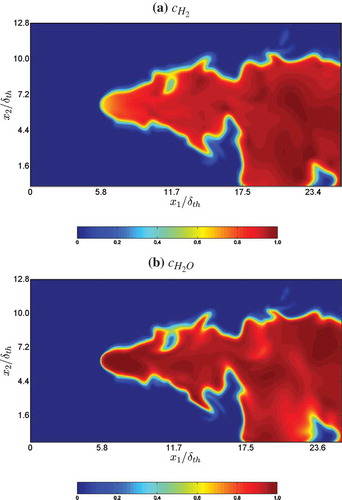
The distributions of reaction progress variables based on H₂ and H₂O mass fractions (i.e., and ) at the central mid-plane at when the statistics are extracted are shown in Figures 1a and 1b, respectively. It is evident from the reaction progress variable distributions in Figures 1a and 1b that the chemical reaction takes place in a continuous (i.e., unbroken) thin region separating unburned and burned gases, indicating flamelet regime of combustion (Peters, 2000), where the SDR closures discussed in this article are meant to be valid.

Figure 1. Distributions of on mid-plane for (a) and (b) when the statistics were extracted.

Algebraic closure of SDR

The performance of the algebraic SDR closure based on simple chemistry has been shown elsewhere (Gao et al., 2014a, 2014b; Ma et al., 2014a) and thus are not repeated here. A wrinkling factor can be defined in the following manner in order to assess the volume-integrated behavior of the SDR closure (Dunstan et al., 2013; Gao et al., 2014a, 2014b, 2015a):

(8)

The variation of with for SDRs for different reaction progress variable definitions based on H₂ and H₂O mass fractions (i.e., and ) is shown in Figure 2. It can be seen from Figure 2 that increases with increasing , indicating that the sub-grid contribution to SDR increases with an increase in LES filter width. It can further be seen from Figure 2 that for the SDR based on assumes greater values than the SDR of . This is consistent with previous findings (Gao et al., 2014a, 2014b, 2015a), which indicated that assumes high values for small values of (e.g., and ). The slope of the best-fit straight line, which approximates the variation of with for large filter widths (i.e., ), provides an indication that can, in principle, be expressed in terms of a power law as: , where is the normalized inner cut-off scale, which can be obtained from the abscissa of the intersection point of the best-fit straight line with . It can be seen from Figure 2 that remains of the order of for variations based on both and . Thus, a higher value of bears the signature of greater value of and accordingly for based on is greater than that based on (i.e., and 1.166 for based on and , respectively). The increase in with decreasing is consistent with previous findings (Gao et al., 2014a, 2014b). Although the power law can be used to mimic the variation of with , it cannot adequately capture the local behavior of Favre-filtered SDR due to multi-fractal nature of SDR, and interested readers are referred to Dunstan et al. (2013), Gao et al. (2014a, 2015a), and Langella et al. (2015) for further discussion on this behavior. The power law will not be discussed further in this article. From the foregoing, it is evident that an algebraic closure of SDR is ideally required to capture to the correct variation of with irrespective of the definition of reaction progress variable along with capturing the local variation of .

Figure 2. Variations of wrinkling factor based on volume averaged quantities with normalized filter width on a log-log plot along with the prediction of Eq. (2) for and .

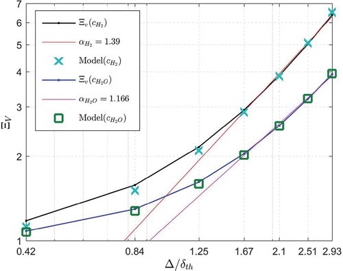
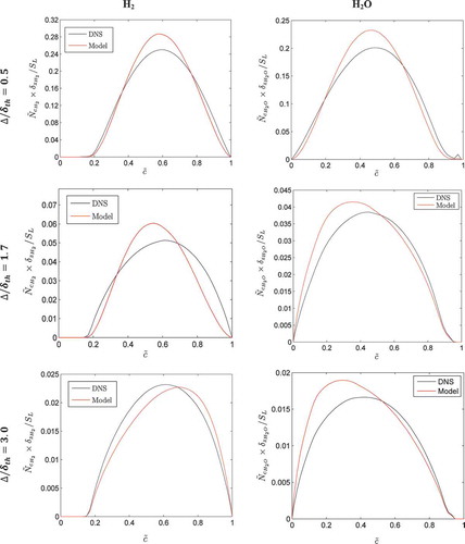
Figure 2 shows that Eq. (2) satisfactorily captures the behavior of the wrinkling factor for both reaction progress variable definitions based on H₂ and H₂O mass fractions. The variation of mean value of normalized Favre-filtered SDR (i.e., , where is the Zel’dovich flame thickness with being the unburned gas diffusivity for reaction progress variable) conditional on shown in Figure 3 for , and for both reaction progress variable definitions based on H₂ and H₂O mass fractions (i.e., and ). It can be seen from Figure 3 that Eq. (2) satisfactorily predicts both the qualitative and quantitative behaviors of SDR across the flame brush for both choices of reaction progress variable. The observations based on Figures 2 and 3 reveal that the algebraic closure given by Eq. (2) satisfactorily predicts both volume-averaged and local behaviors of Favre-filtered SDR for a range of different filter widths for different choices of reaction progress variable in the context of detailed chemistry-based DNS data. It was shown earlier (Gao et al., 2014a, 2014b, 2015a) that the model given by Eq. (2) satisfactorily captures both the local and volume-averaged behaviors of Favre-filtered SDR in the context of simple chemistry DNS. Thus, the evidence suggests that the algebraic model given by Eq. (2) provides a robust closure for Favre-filtered SDR for both simple and detailed chemistry, and this inference was also supported by actual LES simulations (Butz et al., 2015; Ma et al., 2014a).

Figure 3. Variation of mean values of normalized SDR (

) conditional on across the flame brush along with the predictions of Eq. (2) (

) for (1st row), (2nd row), and (3rd row) for (1st column) and (2nd column).

Statistical behavior of the terms of the SDR transport equation

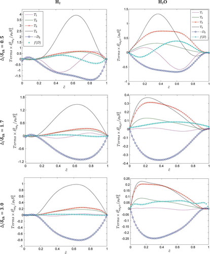
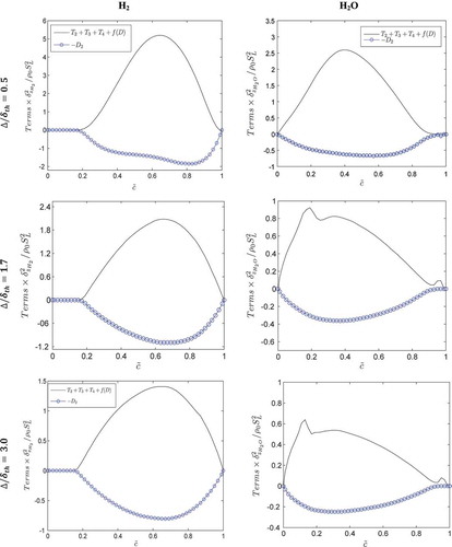
The satisfactory performance of Eq. (2) can be justified in terms of statistical behaviors of the unclosed terms of the SDR transport equation [i.e., Eq. (5)]. The variation of the mean values of , and conditional on is shown in Figure 4 for , , and . It can be seen that the magnitude of remains smaller than that of the other terms in all cases for all filter widths irrespective of the choice of the definition of reaction progress variable. This tendency strengthens further with increasing , which is consistent with the scaling estimates presented in Table 1, because both and increase with increasing (Dunstan et al., 2013; Gao et al., 2014a; Ma et al., 2014a). The molecular dissipation term remains the major sink term, whereas the density variation term acts as a source term for all cases for all filter widths irrespective of the choice of the definition of reaction progress variable. For thermo-diffusively neutral (i.e., ) globally adiabatic flames, can be expressed as , which yields . As dilatation rate remains predominantly positive in premixed flames, the contributions of remain positive for the cases with reaction progress variable Lewis number close to unity (i.e., ). Although the relation does not strictly hold for , the qualitative behavior of is expected to be similar to and, thus, continues to behave as a source term even for the choices of for which . According to the scaling analyses by Swaminathan and Bray (2005) and Gao et al. (2014b), the order of magnitude of is expected to be comparable to , and (see Table 1), which was previously confirmed previously using simple chemistry DNS data (Chakraborty et al., 2008a; Chakraborty and Swaminatthan, 2010, 2013; Gao et al., 2014b). For both choices of reaction progress variable the magnitude of remains about 20% of the magnitudes of and for all filter widths shown in Figure 4. The magnitude of depends on the correlations between , , and [see Eq. (6b)] and in the context of detailed chemistry these correlations are likely to be weaker than in the case of simple chemistry because the locations of high heat release (i.e., the locations of high ) are not necessarily coincident with the locations of high values of for detailed chemistry cases (unlike simplified chemistry cases) when is defined based on major reactants/products mass fractions especially in the presence of differential diffusion as in the case of H₂-air flames. This along with small values of heat release parameter (i.e., ) acts to reduce the magnitude of in comparison to the magnitudes of and in the case considered here.

Figure 4. Variations of , , , , , and conditionally averaged in bins of for (1st row), (2nd row), and (3rd row) for (1st column) and (2nd column). All of the terms are normalized with respect to the value of .

The mean value of the scalar-turbulence interaction term conditional on acts as a leading order source term for both H₂ and H₂O based reaction progress variables (i.e., and ). The contribution of can be expressed as (Chakraborty and Swaminathan, 2007; Chakraborty et al., 2009; Swaminathan and Grout, 2006): , where , and are the most extensive, intermediate, and the most compressive principal strain rates; the angles between the corresponding eigenvectors with are given by , and , respectively. The scalar gradient aligns with when the strain rate induced by flame normal acceleration overcomes turbulent straining , and vice versa (Chakraborty and Swaminathan, 2007; Chakraborty et al., 2009). The strain rate scales as , where is expected to decrease with increasing (Chakraborty et al., 2009). Scaling as (Meneveau and Poinsot, 1991) and (Tennekes and Lumley, 1972) yields: and , respectively. Turbulent straining dominates over the strain rate due to flame normal acceleration throughout the flame brush in this V-flame case due to the small value of , which leads to a predominant alignment of with leading to positive values of throughout the flame brush for both definitions of reaction progress variable (i.e., and ). It can be seen from Figure 4 that the relative magnitude of is greater in the case of H₂O mass fraction based progress variable (i.e., ) than in the case of H₂ mass fraction based progress variable (i.e., ). The magnitude of conditional mean value of is comparable to that of for H₂O mass fraction based progress variable (i.e., ), whereas conditional mean value of is smaller than that of in the case of H₂ mass fraction-based progress variable (i.e., ). As the Lewis number of H₂ is smaller than H₂O, the extent of alignment of with is stronger for than in the case of . This leads to a stronger positive contribution of in the case of H₂O mass fraction based progress variable (i.e., ) than in the case of H₂ mass fraction based progress variable (i.e., ).

The reaction rate contribution exhibits positive values for the major part of the flame brush before assuming negative values towards the burned gas side for small values of characterized by (e.g., ). However, acts as a leading order source term throughout the flame brush for large filter widths characterized by (e.g., and ) irrespective of the choice of reaction progress variable. The term can alternatively be expressed as: , where is the flame normal direction and is the flame normal vector (Gao et al., 2014b). The quantity assumes negative values for the major part of the flame brush except the burned gas side where is positive. As flamelet assumption remains valid for the flames considered here (Peters, 2000), can be expressed as , where is the sub-filter probability density function. The negative (positive) values of lead to positive (negative) values of when the flame is partially resolved (i.e., , for example ), which can be confirmed by Figure 4. For , the flame is completely unresolved and thus the sub-filter volume includes more positive samples with high magnitudes of than the negative samples, which are confined only in a small region within the flame front (i.e., only towards the trailing edge of the flame). This leads to predominantly positive values of throughout the flame brush for (e.g., and ; see Figure 4).

The mean contribution of the diffusivity gradient term conditional on assumes negative values towards the unburned gas side but exhibits positive values towards the burned gas side when the flame is partially resolved (i.e., , for example ) and the reaction progress variable is defined based on H₂O mass fraction. However, the mean value of conditional on assumes positive (negative) values towards the unburned (burned) gas side of the flame brush for when the reaction progress variable is defined based on H₂ mass fraction. The mass diffusivities of H₂ and H₂O and their temperature dependences are different and thus the distributions of with are different for different choices of the reaction progress variable. Figure 4 shows that mean value of conditional on remains positive and its magnitude remains comparable to that of for in this V-flame case for large filter widths where the flame is completely unresolved (e.g., and ). However, the mean value of conditional on remains negligible in comparison to the magnitudes of , and for reaction progress variable based on H₂ mass fraction.

It can further be seen from Figure 4 that the magnitudes of the terms , , and decrease with increasing . This is due to the convolution operation associated with LES filtering. The weighted averaging process associated with LES filtering includes an increasingly large number of samples with negligible magnitudes arising from the unburned and fully burned regions with increasing and thus the magnitudes of , , and decrease with an increase in . Furthermore, the magnitudes of terms , , and remain consistent with the scaling estimates presented in Table 1.

The variations of the normalized mean values of and are shown in Figure 5 for , , and . It is evident from Figure 5 that an approximate equilibrium is maintained between and for (e.g., and ). However, such equilibrium is not so prominent for the filter widths where the flame is partially resolved (e.g., ). It is worth noting that the expression for in Eq. (2) is derived based on the assumption that an approximate equilibrium is maintained between the terms and (Chakraborty and Swaminathan, 2011; Gao et al., 2014a, 2014b, 2015a). Figure 5 indicates that this assumption holds true for (e.g., and ) and thus Eq. (2) satisfactorily predicts SDR . Although the equilibrium between the terms and is not maintained for , where the flame is partially resolved (e.g., ), the resolved part remains the major contributor to the SDR , and in Eq. (2) attains a value close to zero when the flame is partially resolved and thus the inaccuracy incurred by evaluating the sub-grid part of SDR (i.e., ) does not have any major implication on the performance of the model given by Eq. (2) for , which can be substantiated from Figures 2 and 3.

Figure 5. Variations of and conditionally averaged in bins of for (1st row), (2nd row), and (3rd row) for (1st column) and (2nd column). All of the terms are normalized with respect to the corresponding value of .

Transport equation-based SDR closure

It can be seen from Eq. 6a that the sub-grid flux of SDR (i.e., ) needs to be properly modeled to close the turbulent transport term . The sub-grid flux of SDR is often modeled using a gradient hypothesis as (Jones and Musogne, 1988):

(10)

where is the sub-grid scale eddy diffusivity. Several previous analyses (Chakraborty and Cant, 2009b; Chakraborty and Swaminathan, 2010; Veynante et al., 1997) indicated that turbulent flux of scalar gradients (e.g., FSD and SDR) exhibits counter-gradient (gradient) transport for the flames, where counter-gradient (gradient) transport is observed for . Furthermore, a previous analysis (Gao et al., 2014b) indicated that the turbulent transport term can be scaled as and the flux can be taken to scale with (i.e., ) for . Gao et al. (2015b) and Gao and Chakraborty (2016) have recently extended a RANS model proposed by Chakraborty and Swaminathan (2013) for the purpose of modeling in the context of LES, which is referred to as the FLUXG model in Table 2. In the FLUXG model, is the ith component of the resolved flame normal vector for LES; , , and are the model parameters. This parameterization of assumes an asymptotic value for large values of (i.e., ). For non-unity Lewis number flames, the non-dimensional temperature becomes significantly different from the reaction progress variable , which alters the distribution of heat release and thermal expansion within the flame brush in comparison to the flames. This behavior is mimicked here by introducing dependence of the model parameter (Gao and Chakraborty, 2016). In the expression of FLUXG model, the first term on the right-hand side is primarily responsible for the effects of flame normal acceleration due to heat release, whereas the last term on the right-hand side of the FLUXG model represents turbulent transport according to conventional gradient hypothesis. Moreover, the first and second terms on the right-hand side of the FLUXG model satisfy the scaling estimates of provided in Table 1.

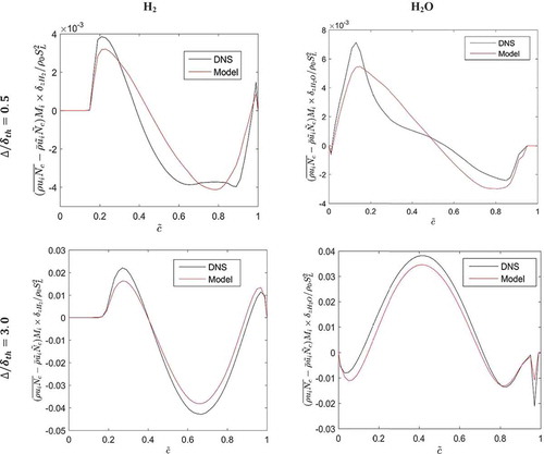
The predictions of according to the FLUXG model are compared to the corresponding quantity extracted from DNS data for and in Figure 6 for different progress variable definitions. It can be seen from Figure 6 that the FLUXG model reasonably captures both qualitative and quantitative behaviors of when and are used in for H₂ and H₂O mass fraction based reaction progress variables (i.e., and ), respectively.

Figure 6. Variations of conditionally averaged in bins of along with the prediction of the FLUXG model for (1st row) and (2nd row) for (1st column) and (2nd column).

It is worth noting that the sub-grid flux of (i.e., ) itself needs modeling in LES, and thus the modeling of and depends on the closure of . The modeling of is beyond the scope of current analysis and interested readers are referred to recent investigations by Gao et al. (2015c, 2015d) for further discussion on the closure of .

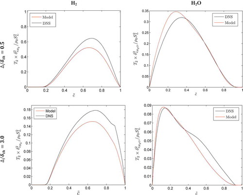
Gao et al. (2015b) and Gao and Chakraborty (2016) recently proposed a model for and validated it with the help of simple chemistry DNS data, which is referred to as the T2G model in Table 2. It can be seen from Table 1 that the magnitude of is expected to increase with decreasing due to the strengthening of heat release effects as a result of enhanced burning rate for small values of Lewis number and this effect is accounted for by in the T2G model (Gao and Chakraborty, 2016), which is consistent with the scaling estimates presented in Table 1. The predictions of the T2G model for H₂ and H₂O mass fraction based reaction progress variables (i.e., and ) are shown in Figure 7 for and . Figure 7 shows that the T2G model reasonably captures both qualitative and quantitative behaviors of when and are used in (see Table 2) for H₂ and H₂O mass fraction based reaction progress variables, respectively.

Figure 7. Variations of conditionally averaged in bins of along with the prediction of the T2G model for (1st row) and (2nd row) for (1st column) and (2nd column). All of the terms are normalized with respect to the corresponding value of .

The variations of the mean values of conditional on are shown in Figure 8 for and . The scaling estimates of the resolved and sub-grid part of have been provided in Table 1 (Gao et al., 2014b), which reveals that these scaling estimates are dependent of the Lewis number. Interested readers are referred to previous analyses (Chakraborty et al., 2009; Chakraborty and Swaminathan, 2010; Gao et al., 2014b) for further discussion on effects on . Gao et al. (2015b) and Gao and Chakraborty (2016) utilized the scaling estimates presented in Table 1 to propose a model for , which is referred to as the T3G model in Table 2, where and are the model parameters and is the density-weighted local sub-grid Damköhler number. It is worth noting that the terms and in the T3G model are consistent with scaling estimates T3S1 and T3S2 presented in Table 1. The term represents the alignment of with under the action of flame normal acceleration, whereas accounts for the alignment of with under turbulent straining. The sub-grid Karlovitz number dependence of accounts for the weakening of the effects of flame normal acceleration with increasing Karlovitz number as the reacting flow field exhibits some attributes of passive scalar mixing for large values of Karlovitz number (Peters, 2000). The symbol in the T3G model is a bridging function in terms of , which ensures that for and approaches to when the flow is fully resolved:

(11)

Figure 8. Variations of conditionally averaged in bins of along with the prediction of the T3G model for (1st row) and (2nd row) for (1st column) and (2nd column). All of the terms are normalized with respect to the corresponding value of .

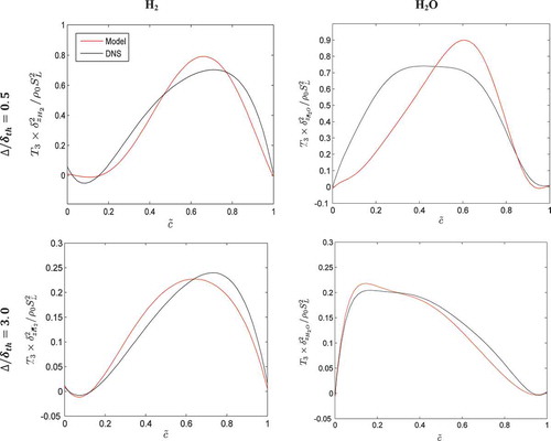
In the T3G model, addresses the strengthening of alignment with under strong actions of flame normal acceleration in the flames with small values of Lewis number, which is consistent with the scaling estimates presented in Table 1 (Gao et al., 2014a). The presence of helps the T3G model to capture the qualitative behavior of across the flame brush. The predictions of the T3G model are compared to extracted from DNS data in Figure 8, which shows that the T3G model reasonably captures both qualitative and quantitative behaviors of when and ( and ) are used in () for H₂ and H₂O mass fraction based progress variables, respectively.

The variations of the mean values of conditional on are shown in Figure 9 for and . The scaling estimates of the resolved (i.e., , , and ) and sub-grid (i.e., , , and ) components of , and are provided in Table 1 according to Gao et al. (2014b). Gao et al. (2015b), and Gao and Chakraborty (2016) utilized to model together for unity Lewis number flames by extending an existing RANS model (Chakraborty et al., 2008a; 2009; Chakraborty and Swaminathan, 2010, 2013; Mantel and Borghi, 1994), which is referred to as the T4D2FG model in Table 2. The involvement of in the T4D2FG model is required for capturing the qualitative behavior of across the flame brush, whereas approaches unity for small values of as the terms get fully resolved (i.e., ). The change in sign of with increasing has been accounted for by . Table 1 suggests that the magnitude of is expected to increase with a decrease in Lewis number . The increased magnitude of for small values of is addressed by dependence of the model parameter (i.e., ). 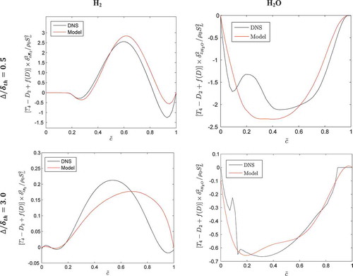The prediction of the T4D2FG model is shown in Figure 9, which demonstrates that the T4D2FG model reasonably captures both qualitative and quantitative behaviors of when and ( and ) are used in () for H₂ and H₂O mass fraction based progress variables, respectively.

Figure 9. Variations of conditionally averaged in bins of along with the predictions of the T4D2FG model for (1st row) and (2nd row) for (1st column) and (2nd column). All of the terms are normalized with respect to the corresponding value of .

Conclusions

The algebraic and transport equation based closures of Favre-filtered SDR in the context of LES, which were previously proposed based on simple chemistry DNS data, have been assessed in the current analysis based on a detailed chemistry DNS dataset of a turbulent stoichiometric H₂-air V flame. The SDR statistics and closure in the context of detailed chemistry DNS data have been assessed for different choices of reaction progress variable. It has been found that Lewis number of reaction progress variable and the choices of itself have noticeable influences on the statistical behavior of the unclosed terms of transport. A recently proposed algebraic closure for , which was previously validated for simple chemistry DNS data for different values of , has been found to yield satisfactory prediction also for detailed chemistry DNS data for different choices of reaction progress variable . The models for the unclosed terms of the SDR transport equation, which were previously proposed based on simple chemistry DNS data, have also been found to satisfactorily predict the unclosed terms obtained from explicitly filtered DNS data for a range of for different choices of reaction progress variable in the context of detailed chemistry DNS data. Although the proposed algebraic and transport equation-based closures have been demonstrated to provide satisfactory performance based on the assessment with respect to explicitly filtered DNS data, it is still essential to implement these models in actual LES simulations because the input parameters (e.g., sub-grid turbulent velocity fluctuation ) to the combustion models often themselves need closures. Thus, the sensitivity of the combustion model predictions on the modeling inaccuracy of input parameters cannot be assessed based solely on model validation with respect to DNS data. This needs implementation of the models, which have been identified based on the validation using DNS data, in actual LES simulations for the purpose of a-posteriori assessment. However, a-posteriori assessment of the models discussed in this article is beyond the scope of this analysis but it is worth mentioning that numerical inaccuracies interact with modeling errors in a complex manner in actual LES simulations so a-posteriori analyses do not assess the models in isolation and are specific to the numerical schemes used in the computer code employed for LES simulations. Ma et al. (2014a), Butz et al. (2015), and Langella et al. (2015) implemented the algebraic SDR closure discussed in this article for LES simulations of premixed turbulent combustion in rectangular dumped-combustor and bluff body stabilized flames (i.e., ORACLE and VOLVO rigs), turbulent swirl flame (i.e., TECFLAM), and Bunsen-burner configurations and reported satisfactory agreement with experimental data based on a-posteriori assessment. However, this algebraic SDR closure and the closures of the unclosed terms of the SDR transport equation need to be validated further based on actual LES simulations. Further validation of these models will form the basis of future investigations.

Acknowledgments

N.C. is grateful to Mr. Jiawei Lai of Newcastle University for his help while preparing this manuscript.

Funding

The financial assistance of the Engineering and Physical Science (EPSRC) research council of the UK (EP/I028013/1 and EP/K025163/1) and computational support of ARCHER and N8 are gratefully acknowledged. Sandia is a multi-program laboratory operated by Sandia Corporation, a Lockheed Martin Company, for the United States Department of Energy under Contract DE-AC04-94AL85000.

Additional information

Funding

The financial assistance of the Engineering and Physical Science (EPSRC) research council of the UK (EP/I028013/1 and EP/K025163/1) and computational support of ARCHER and N8 are gratefully acknowledged. Sandia is a multi-program laboratory operated by Sandia Corporation, a Lockheed Martin Company, for the United States Department of Energy under Contract DE-AC04-94AL85000.

References

- Ahmed, I., and Swaminathan, N. 2013. Simulation of spherically expanding turbulent premixed flames. Combust. Sci. Technol., 185, 1509.
- Bilger, R.W. 2004. Some aspects of scalar dissipation. Flow Turbul. Combust., 72(2–4), 93.
- Boger, M., Veynante, D., Boughanem, H., and Trouvé, A. 1998. Direct numerical simulation analysis of flame surface density concept for large eddy simulation of turbulent premixed combustion. Proc. Combust. Inst., 27, 917.
- Bray, K.N.C. 1980. Turbulent flows with premixed reactants. In P.A. Libby and F.A. Williams (Eds.), Turbulent Reacting Flows, Springer Verlag, Berlin, Heidelburg, New York, pp. 115–183.
- Butz, D., Gao, Y., Kempf, A.M., and Chakraborty, N. 2015. Large eddy simulations of a turbulent premixed swirl flame using an algebraic scalar dissipation rate closure. Combust. Flame, 162, 3180.
- Chakraborty, N., and Cant, R.S. 2009a. Direct numerical simulation analysis of the flame surface density transport equation in the context of large eddy simulation. Proc. Combust. Inst., 32, 1445.
- Chakraborty, N., and Cant, R.S. 2009b. Effects of Lewis number on scalar transport in turbulent premixed flames. Phys. Fluids, 21, 035110.
- Chakraborty, N., and Cant, R. S. 2011. Effects of Lewis number on flame surface density transport in turbulent premixed combustion. Combust. Flame, 158, 1768.
- Chakraborty, N., Champion, M., Mura, A., and Swaminathan, N. 2011. Scalar dissipation rate approach to reaction rate closure. In N. Swaminathan and K.N.C. Bray (Eds.), Turbulent Premixed Flame, 1st ed., Cambridge University Press, Cambridge, UK, pp. 76–102.
- Chakraborty, N., Hawkes, E.R., Chen, J.H., and Cant, R.S. 2008b. The effects of strain rate and curvature on surface density function transport in turbulent premixed methane–air and hydrogen–air flames: A comparative study. Combust. Flame, 154, 259.
- Chakraborty, N., and Klein, M. 2008. A priori direct numerical simulation assessment of algebraic flame surface density models for turbulent premixed flames in the context of large eddy simulation. Phys. Fluids, 20, 085108.
- Chakraborty, N., Klein, M., and Swaminathan, N. 2009. Effects of Lewis number on reactive scalar gradient alignment with local strain rate in turbulent premixed flames. Proc. Combust. Inst., 32, 1409.
- Chakraborty, N., Rogerson, J.W., and Swaminathan, N. 2008a. A priori assessment of closures for scalar dissipation rate transport in turbulent premixed flames using direct numerical simulation. Phys. Fluids, 20, 045106.
- Chakraborty, N., Rogerson, J.W., and Swaminathan, N. 2010. The scalar gradient alignment statistics of flame kernels and its modelling implications for turbulent premixed combustion. Flow Turbul. Combust., 85(1), 25.
- Chakraborty, N., and Swaminathan, N. 2007. Influence of Damköhler number on turbulence-scalar interaction in premixed flames, Part I: Physical insight. Phys. Fluids, 19, 045103.
- Chakraborty, N., and Swaminathan, N. 2010. Effects of Lewis number on scalar dissipation transport and its modelling implications for turbulent premixed combustion. Combust. Sci. Technol., 182, 1201.
- Chakraborty, N., and Swaminathan, N. 2011. Effects of Lewis number on scalar variance transport in premixed flames. Flow Turbul. Combust., 87, 261.
- Chakraborty, N., and Swaminathan, N. 2013. Effects of turbulent Reynolds number on the scalar dissipation rate transport in turbulent premixed flames in the context of Reynolds averaged Navier Stokes simulations. Combust. Sci. Technol., 185, 676.
- Charlette, F., Meneveau, C., and Veynante, D. 2002a. A power-law flame wrinkling model for LES of premixed turbulent combustion. Part I: Nondynamic formulation and initial tests. Combust. Flame, 131, 159.
- Charlette, F., Meneveau, C., and Veynante, D. 2002b. A power-law flame wrinkling model for LES of premixed turbulent combustion. Part II: Dynamic formulation. Combust. Flame, 131, 181.
- Dong, H.Q., Robin, V., Mura, A., and Champion, M. 2013. Analysis of algebraic closures of the mean scalar dissipation rate of the progress variable applied to stagnating turbulent flames. Flow Turbul. Combust., 90, 301.
- Dopazo, C. 1994. Recent developments in PDF methods. In P.A. Libby and F.A. Williams (Eds.), Turbulent Reacting Flows, Springer Verlag, Berlin, Heidelburg, New York, pp. 375–474.
- Dunstan, T., Minamoto, Y., Chakraborty, N., and Swaminathan, N. 2013. Scalar dissipation rate modelling for large eddy simulation of turbulent premixed flames. Proc. Combust. Inst., 34, 1193.
- Freitag, M. 2007. On the simulation of premixed combustion taking into account variable mixtures. PhD thesis. Technische Universität, Darmstadt, Germany.
- Gao, Y., and Chakraborty, N. 2016. Modelling of Lewis number dependence of scalar dissipation rate transport for large eddy simulations of turbulent premixed combustion. Numer. Heat Transfer, Part A, 69, 1201.
- Gao, Y., Chakraborty, N., and Klein, M. 2015c. Assessment of sub-grid scalar flux modelling in premixed flames for large eddy simulations: A-priori direct numerical simulation. Eur. J. Mech. B. Fluids, 52, 97.
- Gao, Y., Chakraborty, N., and Klein, M. 2015d. Assessment of the performances of sub-grid scalar flux models for premixed flames with different global Lewis numbers: A direct numerical simulation analysis. Int. J. Heat Fluid Flow, 52, 28.
- Gao, Y., Chakraborty, N., and Swaminathan, N. 2014a. Algebraic closure of scalar dissipation rate for large eddy simulations of turbulent premixed combustion. Combust. Sci. Technol., 186, 1309.
- Gao, Y., Chakraborty, N., and Swaminathan, N. 2014b. Scalar dissipation rate transport in the context of large eddy simulations for turbulent premixed flames with non-unity Lewis number. Flow Turbul. Combust., 93, 461.
- Gao, Y., Chakraborty, N., and Swaminathan, N. 2015a. Dynamic scalar dissipation rate closure for large eddy simulations of turbulent premixed combustion: A direct numerical simulations analysis. Flow Turbul. Combust, 95, 775.
- Gao, Y., Chakraborty, N., and Swaminathan, N. 2015b. Scalar dissipation rate transport and its modelling for large eddy simulations of turbulent premixed combustion. Combust. Sci. Technol., 187(3), 362.
- Gutheil, E., Balakrishnan, G., and Williams, F.A. 1993. Reduced kinetic mechanisms for applications in combustion systems. In N. Peters and B. Rogg (Eds.), Lecture Notes in Physics, Springer Verlag, New York, pp. 177–195.
- Hawkes, E.R., and Cant, R.S. 2000. A flame surface density approach to large eddy simulation of premixed turbulent combustion. Proc. Combust. Inst., 28, 51.
- Hawkes, E.R., and Cant, R.S. 2001. Implications of a flame surface density approach to large eddy simulation of turbulent premixed combustion. Combust. Flame, 126, 1617.
- Hawkes, E.R., and Chen, J.H. 2005. Evaluation of models for flame stretch due to curvature in the thin reaction zones regime. Proc. Combust. Inst., 30, 647.
- Hawkes, E.R., and Chen, J.H. 2006. Comparison of direct numerical simulation of lean premixed methane–air flames with strained laminar flame calculations. Combust. Flame, 144, 112.
- Hernandez-Perez, F.E., Yuen, F.T.C., Groth, C.P.T., and Gülder, Ö.L. 2011. LES of a laboratory-scale turbulent premixed Bunsen flame using FSD, PCM-FPI and thickened flame models. Proc. Combust. Inst., 33, 1365.
- Jones, W.P., Marquis, A.J., and Prasad, V.N. 2012. LES of a turbulent premixed swirl burner using the Eulerian stochastic field method. Combust. Flame, 159, 3079.
- Jones, W.P., and Musonge, P. 1988. Closure of the Reynolds stress and scalar flux equations. Phys. Fluids, 31, 3589.
- Katragadda, M., Chakraborty, N., and Cant, R.S. 2012. A-priori DNS assessment of wrinkling factor based algebraic flame surface density models in the context of large eddy simulations for non-unity Lewis number flames in the thin reaction zones regime. J. Combust., 2012, 794671.
- Kee, R.J., Dixon-Lewis, G., Warnatz, J., Coltrin, M.E., and Miller, J.A. 1986. A Fortran computer code package for the evaluation of gas-phase multicomponent transport properties. Report No. SAND86-8246. Sandia National Laboratories, Albuquerque, NM.
- Kee, R., Rupley, J.F.M., and Miller, J.A. 1989. Chemkin-II: A Fortran chemical kinetics package for the analysis of gas phase chemical kinetics. Report No. SAND89-8009B. Sandia National Laboratories, Albuquerque, NM.
- Klimenko, A.Y., and Bilger, R.W. 1999. Conditional moment closure for turbulent combustion. Prog. Energy Combust. Sci., 25, 595.
- Kolla, H., Rogerson, J., Chakraborty, N., and Swaminathan, N. 2009. Prediction of turbulent flame speed using scalar dissipation rate. Combust. Sci. Technol., 181, 518.
- Kolla, H., and Swaminathan, N. 2010a. Strained flamelets for turbulent premixed flames. I: Formulation and planar flame results. Combust. Flame, 157, 943.
- Kolla, H., and Swaminathan, N. 2010b. Strained flamelets for turbulent premixed flames. II: Laboratory flame results. Combust. Flame, 157, 1274.
- Kuenne, G., Ketelheun, A., and Janicka, J. 2011. LES modeling of premixed combustion using a thickened flame approach coupled with FGM tabulated chemistry. Combust. Flame, 158, 1750.
- Langella, I., Swaminathan, N., Gao, Y., and Chakraborty, N. 2015. Assessment of dynamic closure for premixed combustion LES. Combust. Theor. Model., 19, 628.
- Ma, T., Stein, O., Chakraborty, N., and Kempf, A. 2013. A-posteriori testing of algebraic flame surface density models for LES. Combust. Theor. Model., 17, 431.
- Ma, T., Stein, O., Chakraborty, N., and Kempf, A. 2014a. A-posteriori testing of flame surface density transport equation for LES. Combust. Theor. Model., 18, 32.
- Ma, T., Gao, Y., Kempf, A.M., and Chakraborty, N. 2014b. Validation and implementation of algebraic LES modelling of scalar dissipation rate for reaction rate closure in turbulent premixed combustion. Combust. Flame, 161, 3134.
- Mantel, T., and Borghi, R. 1994. New model of premixed wrinkled flame propagation based on a scalar dissipation equation. Combust. Flame, 96(4), 443.
- Meneveau, C., and Poinsot, T. 1991. Stretching and quenching of flamelets in premixed turbulent combustion. Combust. Flame, 86, 311.
- Minamoto, Y., Fukushima, N., Tanahashi, M., Miyauchi, T., Dunstan, T.D., and Swaminathan, N. 2011. Effect of flow-geometry on turbulence scalar interaction in premixed flames. Phys. Fluids, 23, 125107.
- Mura, A., and Borghi, R. 2003. Towards an extended scalar dissipation equation for turbulent premixed combustion. Combust. Flame, 133, 193.
- Mura, A., Tsuboi, K., and Hasegawa, T. 2008. Modelling of the correlation between velocity and reactive scalar gradients in turbulent premixed flames based on DNS data. Combust. Theor. Model., 12, 671.
- Mura, A., Robin, V., Champion, M., and Hasegawa, T. 2009. Small-scale features of velocity and scalar fields of turbulent premixed flames. Flow Turbul. Combust., 82, 339.
- O’Brien, E.E. 1980. The probability density function (PDF) approach to reacting turbulent flows. In P.A. Libby and F.A. Williams (Eds.), Turbulent Reacting Flows, Springer Verlag, Berlin, Heidelburg, New York, pp. 185–218.
- Peters, N. 2000. Turbulent Combustion, Cambridge University Press, Cambridge, UK.
- Pitsch, H., and Duchamp-de-Lageneste, L. 2002. Large-eddy simulation of turbulent premixed combustion using level-set approach. Proc. Combust. Inst., 29, 2001.
- Poinsot, T., and Lele, S.K. 1992. Boundary conditions for direct simulation of compressible viscous flows. J. Comput. Phys., 101, 104.
- Reddy, H., and Abraham, J. 2012. Two-dimensional direct numerical simulation evaluation of the flame surface density model for flames developing from an ignition kernel in lean methane/air mixtures under engine conditions. Phys. Fluids, 24, 105108.
- Rogerson, J.W., and Swaminathan, N. 2007. Correlation between dilatation and scalar dissipation in turbulent premixed flames. In G. Skevis (Ed.), Proceedings of the 3rd European Combustion Meeting, April 11–13, Chania, Greece.
- Sadasivuni, S., Bulat, G., Senderson, V., and Swaminathan, N. 2012. Application of scalar dissipation rate model to Siemens DLE combustors. Paper no. GT2012-68483. Presented at the ASME Turbo Expo 2012, Copenhagen, Denmark, June 11–15.
- Swaminathan, N., and Bray, K.N.C. 2005. Effect of dilatation on scalar dissipation in turbulent premixed flames. Combust. Flame, 143, 549.
- Swaminathan, N., and Grout, R.W. 2006. Interaction of turbulence and scalar fields in premixed flames. Phys. Fluids, 18, 045102.
- Tennekes, H., and Lumley, J.L. 1972. A First Course in Turbulence, MIT Press, Cambridge, MA.
- Veynante, D., and Poinsot, T. 1997. Large eddy simulations of combustion instabilities in turbulent premixed burners. In Annual Research Briefs 1997, Centre for Turbulence Research, Stanford University, Stanford, CA, pp. 253–275.
- Veynante, D., Trouvé, A., Bray, K.N.C., and Mantel, T. 1997. Gradient and countergradient turbulent scalar transport in turbulent premixed flames. J. Fluid Mech., 332, 263.