A Priori Direct Numerical Simulation Modeling of Scalar Dissipation Rate Transport in Head-On Quenching of Turbulent Premixed Flames

ABSTRACT

The statistical behavior and modeling of scalar dissipation rate (SDR) transport for head-on quenching of turbulent premixed flames by an inert isothermal wall have been analyzed in the context of Reynolds averaged Navier–Stokes simulations based on three-dimensional simple chemistry direct numerical simulation (DNS) data. It has been found that the density variation, scalar-turbulence interaction, reaction rate gradient, molecular diffusivity gradient, and molecular dissipation terms, i.e., , and , respectively, act as leading order contributors to the SDR transport away from the wall and the turbulent transport and molecular diffusion terms remain negligible in comparison to the other terms. The leading order contributors to the SDR transport have been found to be in a rough equilibrium away from the wall before the quenching is initiated but this equilibrium is not maintained during flame quenching. The predictions of the existing models for the unclosed terms of the SDR transport equation have been assessed with respect to the corresponding quantities extracted from DNS data. No existing models have been found to predict the near-wall behavior of the unclosed terms of the SDR transport equation. The models, which exhibit the most satisfactory performance away from the wall, have been modified to account for near-wall behavior in such a manner that the modified models asymptotically approach the existing model expressions away from the wall.

KEYWORDS:

• Direct numerical simulation
• Head-on quenching
• Premixed combustion
• Reynolds averagedNavier–Stokes simulation
• Scalar dissipation rate

Introduction

The scalar dissipation rate (SDR) plays a key role in the closure of reaction rate and micro-mixing in premixed turbulent combustion (Bray, 1980). In the context of Reynolds averaged Navier–Stokes (RANS) and large eddy simulations (LES), the SDR is closed using either an algebraic expression in terms of known quantities (Dunstan et al., 2013; Gao et al., 2014, 2015a; Kolla et al., 2009; Mura and Borghi, 2003; Swaminathan and Bray, 2005) or by solving a transport equation (Chakraborty et al., 2008a, 2011; Chakraborty and Swaminathan, 2010, 2011, 2013; Gao et al., 2015b, 2015c; Mantel and Borghi, 1994; Mura et al., 2008, 2009). Some of the aforementioned closures (e.g., Dunstan et al., 2013; Gao et al., 2014, 2015a; Kolla et al., 2009) have already been implemented in RANS and LES of a range of laboratory-scale (Ahmed and Swaminathan, 2014; Butz et al., 2015; Dong et al., 2013; Kolla and Swaminathan, 2010; Langella et al., 2015; Ma et al., 2014; Robin et al., 2010) and industrial (Sadasivuni et al., 2012) configurations, and satisfactory results have been obtained. However, all of the aforementioned modeling of SDR has been carried out for flows away from the wall and the effects of flame quenching by the wall on SDR transport and its modeling are yet to be analyzed in detail. This gap in the open literature has been addressed here by analyzing the SDR transport and its modeling using direct numerical simulations (DNS) data of head-on quenching of turbulent premixed flames by an isothermal inert wall.

To date, limited effort has been directed to the analysis of wall bounded reacting flows using DNS (Alshaalan and Rutland, 1998, 2002; Bruneaux et al., 1996, 1997; Dabireau et al., 2003; Gruber et al., 2010, 2012; Lai and Chakraborty, 2016; Poinsot et al., 1993). Out of the aforementioned DNS analysis, only Bruneaux et al. (1996) and Alshalaan and Rutland (1998) concentrated on the influences of the wall on flame surface density (FSD)-based reaction rate closure of premixed turbulent combustion. Recently, Lai and Chakraborty (2016) modified the SDR-based reaction rate closure by Bray (1980) for the purpose of flame-wall interaction and suggested modifications to an algebraic closure of SDR (Chakraborty and Swaminathan, 2011; Kolla et al., 2009) for near-wall effects in the case of head-on quenching of turbulent premixed flames. Algebraic closures of SDR are derived based on the equilibrium of generation and destruction rates of scalar gradients but such an equilibrium may not be maintained under certain conditions (e.g., low Damköhler number combustion, combustion instability, etc.) and it may be necessary to solve a model transport equation for the SDR under those circumstances. The presence of an isothermal wall significantly affects the fluid dynamics and thermal transport (Alshaalan and Rutland, 1998, 2002; Bruneaux et al., 1996, 1997; Dabireau et al., 2003; Gruber et al., 2010, 2012; Lai and Chakraborty, 2016; Poinsot et al., 1993), which gives rise to the inequality between reaction progress variable and nondimensional temperature (where , , and are the instantaneous dimensional temperature, unburned gas temperature, and adiabatic flame temperature, respectively) even for low Mach number unity Lewis number flames (Alshaalan and Rutland, 1998, 2002; Bruneaux et al., 1996, 1997; Lai and Chakraborty, 2016; Poinsot et al., 1993). Furthermore, turbulence significantly affects the heat flux at the wall (Alshaalan and Rutland, 1998, 2002; Bruneaux et al., 1996, 1997; Dabireau et al., 2003), which is expected to have significant effects on the correlation between reaction rate and scalar gradient, density variation, and scalar gradient alignment with local principal strain rates, which in turn are likely to be manifested in the statistical behavior of the various terms of the SDR transport equation. However, the effects of the wall on the closure of the unclosed terms of the SDR transport equation in the context of RANS have not been analyzed in the existing literature. This deficit is addressed in this article by carrying out three-dimensional (3D) DNS simulations of head-on quenching of statistically planar turbulent premixed flames with different values of Damköhler and Karlovitz numbers (i.e., and ). The modeling of near-wall physics in the context of RANS is also useful for the purpose of LES as the near-wall modeling in LES is often adopted from RANS, and most LES reduces to RANS in the near-wall region. Furthermore, in the present analysis DNS data has been used to address the inadequacies of the model predictions in the near-wall region, and the modifications to the existing models have been suggested so that they work satisfactorily both near to and away from the wall. Thus, the main objectives of the current analysis are:

1. to identify the near-wall effects on the unclosed terms of the SDR transport equation; and

2. to model the near-wall effects on the unclosed terms of the SDR transport equation.

The rest of the article is organized as follows. The mathematical and numerical background of this work will be presented in the next two sections. Following this, the results will be presented and subsequently discussed. The main findings will be summarized and the main conclusions will be drawn in the final section of this article.

Mathematical background

For the present analysis a single-step Arrhenius-type irreversible chemical reaction is considered for the purpose of computational economy as 3D DNS simulation with detailed chemistry remains prohibitively expensive for a detailed parametric analysis (Chen et al., 2009). The scalar field is represented by a reaction progress variable , which can be defined in terms of a suitable product mass fraction in the following manner:

(1)

where the values in the unburned and burned gases are denoted by 0 and , respectively. According to Eq. (1), increases monotonically from zero in the unburned gas to unity in the fully burned products. Bray (1980) derived the following closure for the mean reaction rate of reaction progress variable in terms of SDR in the following manner for high Damköhler number (i.e., ) flames:

(2)

where is the gas density; is the progress variable diffusivity; is the burning mode probability density function (pdf); , , and are the Reynolds averaged, Favre averaged, and Favre fluctuation values of a general quantity ; and the subscript L is used to refer to unstrained laminar flame quantities. The value of remains between 0.7 and 0.9 for typical hydrocarbon-air flames (Bray, 1980).

Although Eq. (2) was originally proposed for high Damköhler number (i.e., ), it was subsequently shown by Chakraborty and Cant (2011) that Eq. (2) remains valid for low Damköhler number (i.e., ) combustion as long as the flamelet assumption holds true. It is evident from Eq. (2) that needs to be modeled in order to close the mean reaction rate . Using transport equation of , i.e., ), it is possible to derive a transport equation of the SDR , which takes the following form (Borghi, 1990; Gao et al., 2014; 2015b, 2015c; Mantel and Borghi, 1994; Mura and Borghi, 2003; Swaminathan and Bray, 2005):

(3a)

where

(3b)

(3c)

(3d)

(3e)

(3f)

(3g)

The terms on the left-hand side of Eq. (3a) represent the effects of unsteadiness and mean advection, respectively. The terms and denote the molecular diffusion and turbulent transport of , respectively. The term is the density variation term due to heat release, whereas the turbulence-scalar interaction term arises from the alignment of with local principal strain rates. The term signifies the chemical reaction contribution to the SDR transport and is the molecular dissipation term. The term arises due to diffusivity gradients. The terms , , , , , and are unclosed and need modeling for transport equation-based closure. The statistical behavior and the modeling of these terms will be discussed in detail in the “Results and Discussion” section of this article.

Numerical implementation

Three-dimensional DNS simulations of head-on quenching of premixed turbulent flames have been carried out using a compressible DNS code, SENGA (Jenkins and Cant, 1999), where the conservation equations of mass, momentum, energy, and reaction progress variable are solved in nondimensional form in a coupled manner. The simulations have been carried out for a domain of size (where is the Zel’dovich flame thickness with and being the thermal diffusivity of unburned gas and unstrained laminar burning velocity, respectively) with the largest side aligned with the mean direction of flame propagation (i.e., –ve -direction here). The simulation domain is discretized using a uniform Cartesian grid of size , ensuring 10 grid points across the thermal flame thickness . Most existing analyses of flame-wall interaction have been carried out for a constant wall temperature boundary condition (Alshaalan and Rutland, 1998, 2002; Bruneaux et al., 1996, 1997; Dabireau et al., 2003; Gruber et al., 2010, 2012; Poinsot et al., 1993). The same approach has been adopted here. Cooling of the walls is necessary in most combustors because the burned gas temperature is often higher than the melting point of the combustor material, and thus the constant wall temperature boundary condition has a practical relevance. A no-slip isothermal inert wall with temperature is taken to be placed on the left-hand side boundary in the -direction and the boundary opposite to the wall is taken to be partially nonreflecting. The mass flux normal to the wall is considered to be zero, which can be written in terms of reaction progress variable as at the wall. The boundaries in and directions are taken to be periodic. The spatial discretization for the internal grid points has been carried out by a 10th-order central difference scheme but the order of differentiation gradually drops to a one-sided 2nd-order scheme at the nonperiodic boundaries (Jenkins and Cant, 1999). The temporal advancement has been carried out by an explicit low storage 3rd-order Runge–Kutta scheme (Wray, 1990). The reactive field is initialized by a steady unstrained planar laminar premixed flame solution. The flame is initially placed at a location where the influence either from or to the wall is marginal (in these cases isosurface for the unstrained planar laminar flame solution is kept at a distance of away from the wall), so that flame gets enough time to evolve in the presence of turbulence before interacting with the wall. For the purpose of initializing the velocity field, an initially homogeneous isotropic field of turbulent velocity fluctuations is generated using a pseudo-spectral method (Rogallo, 1981) following the Batchelor–Townsend spectrum (Batchelor and Townsend, 1948), but the velocity components at the wall , , and are specified to be zero to ensure a no-slip condition. This velocity field is allowed to evolve for an initial eddy turn-over time (i.e., ) before it interacts with the flame.

The initial values of normalized rms turbulent velocity fluctuation , the ratio of turbulent integral length scale to thermal flame thickness for the turbulent velocity field away from the wall are listed in Table 1 along with the corresponding values of Damköhler number , Karlovitz number , and turbulent Reynolds number , where and are the unburned gas density and viscosity, respectively. It can be seen from Table 1 that the cases A, C, and E (B, C, and D) have the same values of () and () is modified to bring about the changes in . The global Lewis number is taken to be unity for all cases considered here (i.e., ). Standard values are chosen for Prandtl number Pr and ratio of specific heats (i.e., and ). For the present analysis, both the heat release parameter and Zel’dovich number are taken to be 6.0 (i.e., and ). The gaseous mixture is assumed to follow the ideal gas laws and the flame Mach number is taken to be 0.014. The simulations for turbulent cases have been carried out for a time when the maximum, mean, and minimum values of wall heat flux assume identical values following the flame quenching. The simulation time remains different for different cases but the simulations for all cases were continued for , where corresponds to 21, 30, 21, 15, and 21 initial eddy turnover times (i.e., ) for cases A–E, respectively. The nondimensional grid spacing next to the wall remains smaller than unity for all turbulent cases (the maximum value of has been found to be 0.93 during the course of the simulation), where , , and are the friction velocity, mean wall shear stress, and kinematic viscosity, respectively. For , the minimum normalized wall normal distance of isosurface has been found to be about for the quenching flames considered here. This implies that the flame does not necessarily quench within the viscous sublayer.

Table 1. List of initial simulation parameters and relevant nondimensional numbers away from the wall.

Case	A	B	C	D	E
	5.0	6.25	7.5	9.0	11.25
	1.67	1.44	2.5	4.31	3.75
	22.0	23.5	49.0	100	110
	0.33	0.23	0.33	0.48	0.33
	8.65	13.0	13.0	13.0	19.5
	1.0	1.0	1.0	1.0	1.0

The DNS data has been ensemble averaged on the transverse plane (i.e., and direction) at a given location for the purpose of extracting Reynolds/Favre averaged quantities. The Reynolds/Favre averaged quantities have been assessed for statistical convergence by comparing the values obtained based on full sample size with the corresponding values evaluated using the distinct half of the domain in the transverse direction, and the agreement has been found to be satisfactory. In the next section, the results based on full sample size will be presented for the sake of conciseness.

Results and discussion

Flame wall interaction

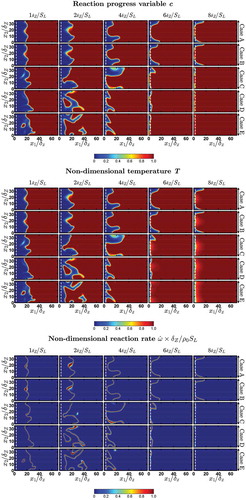
The distributions of reaction progress variable , nondimensional temperature , and nondimensional reaction rate in central plane are shown in Figure 1. For unity Lewis number flame, and are identical to each other under adiabatic low Mach number conditions. This can be observed when the flame is away from the wall prior to the flame quenching. However, the adiabatic condition is not maintained in the case of isothermal boundary condition, and the equality between and does not hold during flame quenching. It can be seen from Figure 1 that the flame wrinkling increases with increasing when the flame is away from the wall. This can be confirmed from the values of normalized flame surface area (where flame area is evaluated using the volume integral and the subscripts T and L are used to refer to turbulent and laminar conditions) presented in Table 2 at different time instants. Table 2 indicates that an increase in promotes a high extent of flame area generation at early times (i.e., ) when the flame is away from the wall. However, a high extent of flame wrinkling for large values of enables the flame elements to reach close to the wall, which in turn leads to early initiation of flame quenching. This can be confirmed from Table 2, which shows that smaller values of have been obtained for the cases with higher initial at later times (e.g., ) due to earlier initiation of flame quenching. The aforementioned behavior can further be confirmed by comparing the distributions of , , and shown in Figure 1. It was shown previously (Lai and Chakraborty, 2016) that the flame quenches once isosurface reaches a certain nondimensional distance normal to the wall and this nondimensional distance is often referred to as the minimum Peclet number (Lai and Chakraborty, 2016; Poinsot et al., 1993). For the unity Lewis number flames considered here the minimum Peclet number for laminar premixed flame head-on quenching is found to be 2.83 (Lai and Chakraborty, 2016), which is consistent with several previous experimental analyses (Huang et al., 1986; Jarosinsky, 1986; Vosen et al., 1984). It was demonstrated by Lai and Chakraborty (2016) that the minimum value of wall Peclet number for head-on quenching of turbulent flames assumes approximately the same values as in the case of the planar laminar flame quenching. Lai and Chakraborty (2016) showed that drops significantly and eventually disappears for , which can be confirmed from the distributions of shown here. Interested readers are referred to Lai and Chakraborty (2016) for further discussion on temporal evolutions of wall heat flux and wall Peclet number in the current configuration for different values of Lewis number.

Table 2. List of normalized flame surface area at different stages of flame quenching for all cases considered here.

	Case A	Case B	Case C	Case D	Case E
1	1.57	1.59	2.79	2.91	4.18
2	1.67	1.60	2.99	3.95	4.77
4	1.77	1.73	2.34	2.39	2.03
6	1.64	1.68	1.43	0.74	0.68
8	1.51	1.53	0.50	0.20	0.12
10	0.86	0.85	0.09	0.03	0.03

Figure 1. Distributions of reaction progress variable , nondimensional temperature , and nondimensional reaction rate contours for cases A–E at , , , , and on central plane. White vertical line indicates .

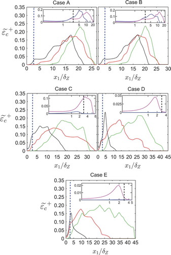
The present article will only concentrate on the closures of the unclosed terms of the SDR transport equation in the case of head-on quenching. Algebraic closure of SDR for head-on quenching has been addressed elsewhere (Lai and Chakraborty, 2016) and will not be repeated here. However, for the sake of completeness, the variation of normalized SDR (i.e., ) with normalized wall normal distance at different time instants is shown in Figure 2 for all cases considered here. It can be seen from Figure 2 that the distribution of broadens with increasing due to an increase in flame wrinkling. A comparison between Figures 1 and 2 reveals that the regions of high reaction progress variable gradient shifts towards the wall and thus the value of , at which the peak value of normalized SDR is obtained, decreases as the flame propagates towards the wall. However, it can be discerned from the reaction progress variable and distributions in Figure 1 that the gradient of disappears upon flame quenching and thus the magnitude of normalized SDR drops significantly once the quenching starts and eventually vanishes (see and ) after flame quenching.

Figure 2. Variation of obtained from DNS data with at t =

;

;

;

; and

for cases A–E. The x₁-axis is shown in log scale for the inset. Blue and black vertical lines indicate .

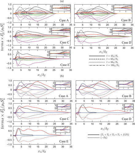
The near-wall behavior of SDR can be understood by examining the terms in the SDR transport equation, i.e., Eq. (3a). The variations of normalized values of the terms on the right-hand side of the SDR transport equation, Eq. (3a), i.e., , , , , , , and , with normalized wall normal distance at different time instants are shown in Figure 3. The following observations can be made from Figure 3 regarding the SDR transport in the near-wall region:

• The terms , , , , and remain the leading order contributors to the SDR transport for all cases. However, the cases with high values of exhibit high magnitudes of these terms.

• The chemical reaction rate term acts as a dominant source away from the wall for all cases considered here. However, the magnitude of drops significantly and eventually vanishes following flame quenching (e.g., .

• The dissipation term acts as the dominant sink for all cases but its magnitude also decreases in the near-wall region as a result of flame quenching.

• The density variation term acts as the second dominant source term away from the wall for all cases. As a result of large heat loss through the wall, the reaction rate vanishes in the near-wall region, which leads to a weak/zero contribution of . However, assumes non-negligible values in the near-wall region because of significant variations of density in this region due to temperature change even in the absence of chemical reaction rate.

• The scalar-turbulence interaction term acts predominantly as a sink term for cases A–D, but this term locally exhibits positive values in case E at early times. However, it assumes negative values as time progresses before vanishing altogether.

• The diffusivity variation term acts as a sink in the near-wall region but this term assumes small positive values away from the wall. This term especially plays the role of a dominant sink in the near-wall region.

• It is evident from Figure 3 that the magnitudes of the molecular diffusion term and the turbulent transport term remain negligible in comparison to the magnitudes of , , , , and .

Figure 3. (a) Variations of

;

;

;

;

;

; and

with at t = , and for cases A–E. (b) Variations of and with at t =

;

;

;

;

; and

for turbulent cases A–E. The terms , , , , , and are normalized using .

Swaminathan and Bray (2005) proposed the following scaling estimates for the unclosed terms of SDR transport equation where the velocity fluctuations and length scales associated with scalar fluctuations are scaled with respect to and , respectively, whereas the gradients of Favre/Reynolds averaged quantities are scaled with respect to integral length scale :

(4a)

An alternative order of magnitude analysis was proposed by Mantel and Borghi (1994) involving the rms turbulent velocity fluctuation and Taylor micro-scale to scale the velocity fluctuations and the gradients of the fluctuating quantities, respectively, according to Tennekes and Lumley (1972):

(4b)

Furthermore, the following scaling estimate for in nonreacting flows can be obtained if the second derivatives of fluctuating quantities are scaled using the Kolmogorov length scale, :

(4c)

Equation (4) indicates that , , , , and are indeed expected to be leading order contributors to the SDR transport, and the magnitudes of and are expected to be negligible in comparison to , , , , and for all cases irrespective of the value of and . This can be substantiated from the behaviors of , , , , and away from the wall for all cases considered here. It can be seen from Figure 3 that for all cases , , , and indeed scale with away from the wall but the magnitudes of all of the unclosed terms of the SDR transport equation decrease once the quenching starts. The magnitude of remains smaller than the terms , and , but it cannot be ignored. However, the magnitudes of all of the terms decay with time once the flame starts to interact with the wall and eventually vanishes after flame quenching. A comparison of the magnitudes of , , and in Figure 3 reveals that the terms , , and in the near-wall region assume negligible values in comparison to , which acts to generate in the near-wall region even where vanishes. Furthermore, it can be seen from Figure 3 that the terms ( and remain roughly in equilibrium when the flame is away from the wall, but such an equilibrium is not maintained once the flame starts to quench.

The modeling of the unclosed terms , , , , , and will be discussed next in this article. Most models for the unclosed terms of the SDR transport equation have been proposed based on a-priori analysis of DNS data in canonical configurations, where there is no mean shear (Chakraborty et al., 2008a, 2009; Chakraborty and Swaminathan, 2010, 2013; Mantel and Borghi, 1994; Mura et al., 2008, 2009). The physical mechanisms that affect the statistical behavior of the various terms of the SDR transport remain mostly unchanged in the presence of the wall because SDR statistics are principally governed by small-scale physics, which are largely independent of mean-scale forcing. For example, dilatation rate is expected to play a key role in turbulent premixed combustion, even for small values of Mach number, irrespective of the presence of the wall. The statistical behavior of the scalar-turbulence interaction term is governed by the alignment of with the local principal strain rates, irrespective of the presence of the wall. Thus, many of the underlying physical mechanisms that affect the SDR transport remain unchanged in the presence of the wall. Therefore, the models that were originally proposed for premixed flames without walls account for some of the physical mechanisms, which are still valid in the presence of the wall. Furthermore, it has recently been found that the models for the unclosed terms of the SDR transport equation, which were originally proposed based on DNS data for turbulent premixed flames without any mean shear, also provide satisfactory predictions for a configuration (i.e., rod-stabilized V-flame), where mean shear is present (Gao et al., 2015c). Thus, the models that were originally proposed based on a-priori DNS analysis of premixed turbulent flames in canonical configuration without walls and mean shear have been considered as a starting point of this analysis because it is easier to modify the existing models to account for near-wall behavior, rather than switching to completely different models in the near-wall region.

Modeling of turbulent transport term

It can be seen from Eqs. (4a) and (4b) that the magnitude of is expected to be negligible in comparison to that of for high values of . Hence, in practical high turbulent flows can be approximated as:

(5a)

In order to model turbulent transport , it is essential to model the turbulent flux , which is often modeled for passive scalar mixing using a gradient flux model for :

(5b)

where is the eddy viscosity, model constant, and is the turbulent Schmidt number with turbulent kinetic energy and its dissipation rate . However, it is well known that turbulent fluxes of the quantities related to turbulent scalar gradient (e.g., FSD and SDR ) exhibit counter-gradient (gradient) when turbulent scalar flux shows counter-gradient (gradient) type behavior (Chakraborty and Cant, 2009; Chakraborty and Swaminathan, 2010, 2013; Veynante et al., 1997). One obtains counter-gradient transport when the velocity jump due to flame normal acceleration dominates over turbulent velocity fluctuations and vice versa (Chakraborty and Cant, 2009; Veynante et al., 1997).

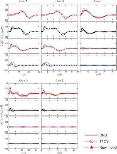
Chakraborty and Swaminathan (2010) proposed a model (referred to as the T1CS model here) for in terms of , which is capable of predicting both gradient and counter-gradient type transport:

(5c)

where the model parameters are given by and (Chakraborty and Swaminathan, 2010). Figure 4 shows that the T1CS model underpredicts the turbulent flux in a region where . As the flame propagates towards the quenching zone, the SDR flux exhibits mainly gradient-type transport. The T1CS model assumes the transition of from a positive to a negative value at by using the factor . This transition is no longer valid in the near-wall region because of predominantly gradient transport and is also due to the absence of the effects of flame normal acceleration as a result of flame quenching. The T1CS model has been revised here in the following manner:

(5d)

Figure 4. Variation of with along with the predictions by the T1CS model and Eq. (5d) (new model) at t =

;

;

; and

for cases A–E.

where , , , and is the minimum Peclet number (i.e., normalized flame quenching distance), which can be obtained from planar laminar flame head-on quenching calculation. The model parameter remains active only in the near-wall region, and it increases the multiplier of and avoids the near-wall underprediction of by the T1CS model. The parameter has been modified in such a manner that it increases the threshold of the transition of from negative to positive value according to the value of Favre-averaged reaction progress variable at the wall . Furthermore, the model parameters and have been parameterized in such a manner that Eq. (5d) approaches Eq. (5c) away from the wall (i.e., ). It can be seen from Figure 4 that the revised model captures both qualitative and quantitative behaviors of both away from and close to the wall.

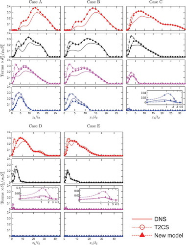
Modeling of density variation term

The fluid density in low Mach number combustion is given by (Bray et al., 1985):

(6a)

The nondimensional temperature can be equated to the reaction progress variable (e.g., ) for globally adiabatic unity Lewis number flames in absence of the wall. Thus, under the aforementioned condition, and can be expressed in terms of and as:

(6b)

Using Eq. (6b), can be expressed in the following manner (Chakraborty et al., 2008a, 2010, 2011; Chakraborty and Swaminathan, 2010; Swaminathan and Bray, 2005):

(6c)

According to above equation, an alternative expression for can be obtained in the following manner for unity Lewis number flames:

(6d)

According to the scaling argument by Swaiminathan and Bray (2005), the terms , , and can be scaled in the following manner:

(6e)

where the velocity fluctuation, gradients of fluctuation, and its mean quantities are scaled using , , and , respectively. Equation (6e) suggests that and become negligible in comparison to for high values of. Consequently, can be taken to scale with (Swaminathan and Bray, 2005). For unity Lewis number flame, the dilatation rate is scaled as (Chakraborty and Swaminathan, 2007a, 2007b, 2013; Chakraborty et al. 2008a, 2010, 2011, 2013; Swaminathan and Bray, 2005), and SDR scales with (Chakraborty et al., 2008a, 2010; Chakraborty and Swaminathan, 2010, 2013; Gao et al., 2015c). The aforementioned scaling arguments have been taken into account in the model proposed by Chakraborty et al. (2008a) for , which takes the following form (T2CS):

(6f)

where is the model parameter with and is the local Karlovitz number (Chakraborty et al., 2008a, 2010; Chakraborty and Swaminathan, 2010, 2013; Gao et al., 2015c). The Karlovitz number dependence of accounts for weakening of magnitude for large values of (Chakraborty et al., 2008a, 2010; Chakraborty and Swaminathan, 2010, 2013; Gao et al., 2015c) due to diminished heat release effects as the broken reaction zones regime is approached (Peters, 2000).

The variations of with normalized wall normal distance at different time instants are shown in Figure 5 for all cases considered here. Figure 5 shows that acts as a source term and assumes higher magnitudes before quenching than after quenching because most of the density variation occurs due to the chemical heat release. The magnitude of also diminishes as reaction rate sharply reduces close to the wall, but nonzero value of has been observed during quenching because of the density variation driven by the temperature change across the thermal boundary layer on the isothermal wall. It can be seen from Figure 5 that the T2CS model satisfactorily predicts extracted from DNS data before flame quenching (i.e., when the flame is away from the wall). However, the T2CS model gives rise to significant overprediction of when flame-wall interaction takes place. Here, the T2CS model has been modified in the following manner to account for flame-wall interaction:

(6g)

Figure 5. Variation of with along with the predictions by the T2CS model and Eq. (6g) (new model) at t =

;

;

; and

for cases A–E. The x₁-axis is shown in log scale for the inset. Insets are not shown in this and subsequent figures when the magnitudes of the normalized quantities are smaller than .

In Eq. (6g), is given by , where and account for the effects of the wall. For unity, Lewis number flames vanish away from the wall but assumes nonzero values only in the near-wall region. This type of dependence was used by Bruneaux et al. (1997) in the context of FSD modeling and the same approach has been adopted here. The exponent rises in the near-wall region, which acts to mimic the reduction of magnitude as a result of weakening of heat release effects arising from flame quenching. It is worth noting that and approach 1.0 and 0.5, respectively, away from the wall and Eq. (6g) becomes identical to the T2CS model, i.e., Eq. (6f), for . It can be seen from Figure 5 that Eq. (6f) reduces the overprediction of , and its predictions are in better agreement with DNS data than the T2CS model in the near-wall region when the flame interacts with the wall. Furthermore, the prediction of Eq. (6g) becomes identical to the T2CS model away from the wall before the flame quenching is initiated.

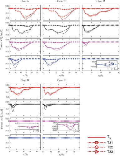
Modeling of the turbulent scalar interaction term

The variations of , , and with at different time instants for cases A–E are shown in Figure 6. It can be seen that and assume predominantly negative values when the flame is away from the wall. The contribution of remains a dominant contribution to . However, as flame interacts with the wall, the magnitude of drops significantly. At the quenching stage, the magnitudes of and gradually become comparable to that of in the near-wall region. The local Damköhler number drops close to the wall due to the combination of the decay of turbulent kinetic energy and a sharp increase of dissipation of turbulent kinetic energy in the near-wall region. This drop in leads to an enhancement in magnitudes of and according to Eq. (4a). At the final stage of quenching, assumes positive values because of predominantly negative values of as a result of the reversal of the direction of the flow (after quenching flow is directed towards the wall in contrast to the flow away from the wall before quenching). The statistical behavior of can also be explained by using the scalar-turbulence interaction contribution :

(7a)

Figure 6. Variation of with along with its components T31, T32, and T33 at t =

;

;

; and

for cases A–E. The x₁-axis is shown in log scale for the inset.

where , , and are the most extensive, intermediate, and most compressive principal strain rates and , , and are the angles between and the eigenvectors associated with , , and , respectively. According to Swaminathan and Bray (2005), the following scaling relation can be obtained:

(7b)

It can be deduced from Eq. (7b) that the quantity remains negligible in comparison to the contributions from , , and . It can be seen from Eq. (7a) that a preferential alignment of with () leads to negative (positive) contributions of and . Several previous analyses (Chakraborty et al., 2009; Chakraborty and Swaminathan, 2007a, 2007b; Swaminathan and Grout, 2006) indicated that aligns preferentially with the most extensive principal strain rate , when the strain rate induced by flame normal acceleration dominates over the effects of turbulent straining . By contrast, a preferential alignment of with occurs when turbulent straining overwhelms the influences of strain rate arising from flame normal acceleration. Scaling and by and , alternatively , respectively yields , alternatively (Chakraborty et al., 2009; Chakraborty and Swaminathan, 2007a, 2007b, 2013), which suggests that is likely overwhelm for large values of and/or . For the cases considered here, dominates over in spite of due to the large value of . Thus, predominantly aligns with for all cases, which predominantly gives rise to negative values of , except at the final stage of flame quenching when assumes positive values close to the wall due to positive values of due to flow direction reversal. From the aforementioned discussion it is clear that the models of components need to account for alignment characteristics with local principal strain rates.

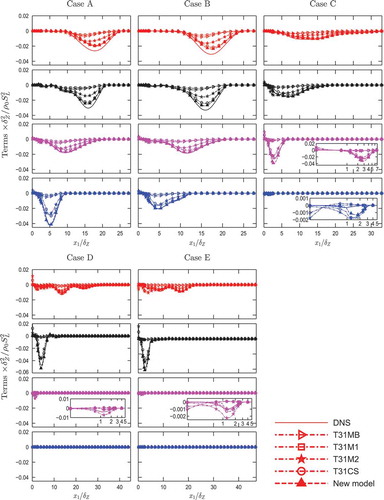
For the present analysis four existing models of have been considered for model comparison, which are listed as:

T31MB (Mantel and Borghi, 1994):

(8a)

T31M1 (Mura et al., 2009):

(8b)

T31M2 (Mura et al., 2009):

(8c)

where is a local flamelet normal vector.

T31CS (Chakraborty and Swaminathan, 2013):

(8d)

where is the local density-weighted Damköhler number, and are the model parameters, and the model parameter is expressed as:

(8e)

It was demonstrated by Chakraborty and Swaminathan (2013) that the T31CS model captures both the qualitative and quantitative behaviors of for a range of values of , , and in the absence of the wall.

The variations of with normalized wall normal distance are shown in Figure 7 along with the predictions of the T31MB, T31M1, T31M2, and T31CS models for different time instants for all cases considered here. All of these models underpredict the magnitude of and the extent of this underprediction is particularly severe for the T31MB and T3M1 models. The agreement of the T3M2 and T3CS model predictions with DNS data remain better than the other models when the flame is away from the wall (i.e., ) and also when the quenching starts. Nonetheless, the T31M2 and T31CS models do not adequately predict extracted from DNS data in the near-wall region. The T31CS model starts to underpredict the DNS data once the quenching is initiated. In order to address this deficiency, the following modification to the T31CS model has been proposed here:

(8f)

Figure 7. Variation of with along with the predictions by the T31MB, T31CS, T31M1, and T31M2 models and Eq. (8f) (new model) at t =

;

;

; and

for cases A–E. The x₁-axis is shown in log scale for the inset.

where and are the model parameters, which account for the wall effects. The model parameter acts to reduce the overprediction of magnitude once the flame starts to interact with the wall (see in Figure 7). The model parameter becomes active in the near-wall region where , and is responsible for damping the magnitude of close to the near-wall region. The term is necessary to accurately predict away from the wall. However, it has a strong dependence on , and changes rapidly in the near-wall region due to the interaction of the flame with the wall. The involvement of in Eq. (8f) reduces this dependence close to the wall. It can be seen from Figure 7 that the model given by Eq. (8f) provides better performance than the other available models and thus is recommended for modeling.

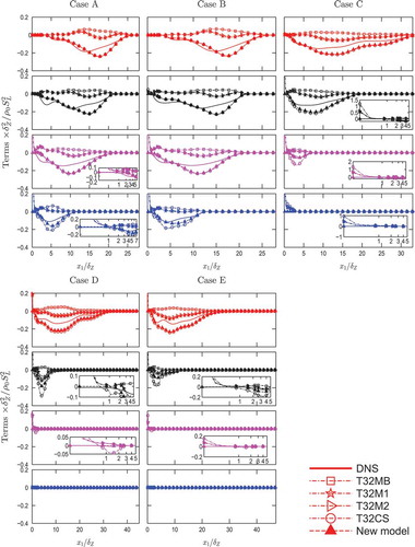
Mantel and Borghi (1994) proposed the following model for (T32MB):

(9a)

where is a model parameter. Mura et al. (2008) proposed the following models for based on a-priori analysis of DNS data for high flames:

(9b)

(9c)

where , , and are the model constants and is the local Damköhler number. Equations (9b) and (9c) will henceforth be referred to as the T32M1 and T32M2 models in this article. Chakraborty and Swaminathan (2010) proposed a model for , which includes nonunity Lewis number effects (T32CS):

(9d)

where , , , and are the model parameters. The term accounts for scalar gradient generation due to preferential alignment between and [see Eq. (7a)]. By contrast, accounts for the destruction of scalar gradient as a result of preferential alignment between and [see Eq. (7a)], and the local Karlovitz number dependence of accounts for weakening of alignment with with increasing Karlovitz number due to diminishing influence of flame normal acceleration for high Karlovitz number combustion. The involvement of in the second term on the right-hand side of Eq. (9d) allows for strengthening of flame normal acceleration with decreasing (Chakraborty et al., 2009; Chakraborty and Swaminathan, 2010). The involvement of ensures that the qualitative behavior of variation with is adequately captured (Chakraborty and Swaminathan, 2010, 2013).

The predictions of the T32MB, T32M1, T32M2, and T32CS models are compared to extracted from DNS data in Figure 8. It can be seen from the variations of with normalized wall normal distance in Figure 8 that the T32MB model fails to predict the negative values of for all cases. The performances of the T32M1 and T32M2 models remain comparable but their predictions remain an order of magnitude smaller than the corresponding quantity extracted from DNS data. The agreement between the T32CS model prediction with DNS data is better than the other models before quenching is initiated (i.e., when the flame remains away from the wall by the wall) in spite of overpredictions of the magnitude of the negative values of for the flames considered here. However, the quantity assumes large values close to the wall (due to augmentation of and decay of in the vicinity of the wall), which leads to severe overprediction of by all of the models in the near-wall region. In order to capture the near-wall behavior of the T32CS model has been modified in the following manner:

(9e)

Figure 8. Variation of with along with the predictions by the T32MB, T32M1, T32M2, and T32CS models and Eq. (9e) (new model) at t =

;

;

; and

for cases A–E . The x₁-axis is shown in log scale for the inset.

Here, the modified parameters are , , and . The parameter is responsible for compensating the overprediction originating from , and it asymptotically approaches unity for . The involvement of in strengthens the damping of the influences of at high values of in the near-wall region. It can be seen from Figure 8 that the new model given by Eq. (9e) captures the quantitative behavior of more satisfactorily than the T32CS model both away from and near to the wall. Furthermore, the modifications suggested in Eq. (9e) reduce the extent of the overprediction of the magnitude of the negative values of in comparison to the T32CS model.

Mantel and Borghi (1994) proposed the following model for :

(10a)

Chakraborty and Swaminathan (2007b) proposed an alternative model for :

(10b)

where , , and are the model parameters. Mura et al. (2009) proposed the following models for :

(10c)

(10d)

(10e)

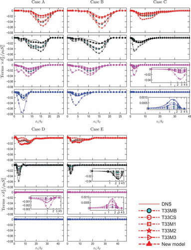
The models given by Eqs. (10c)–(10e) will henceforth be referred to as the T33M1, T33M2, and T33M3, respectively.

The predictions of the T33MB, T33CS, T33M1, T33M2, and T33M3 models are compared with DNS data in Figure 9. It can be seen from Figure 9 that the T33MB model overpredicts the magnitude of the negative contribution of for cases A and B when the flame is away from the wall. However, it performs satisfactorily away from the wall in cases C–E before flame quenching. However, the model T33MB underpredicts the magnitude of in the near-wall region once the flame quenching is initiated. It can be seen from Figure 9 that the T33M1 model satisfactorily predicts for cases A and B when the flame is away from the wall as well as at the quenching stage. The models T33M2 and T33M3 overpredict the magnitude of the negative value of when the flame is away from the wall (e.g., ), nonetheless, the T33M2 model underpredicts whereas the T33M3 model significantly overpredicts the magnitude of during the final stage of quenching.

Figure 9. Variation of with along with the predictions by the T33MB, T33CS, T33M1, T33M2, and T33M3 models and Eq. (10f) (new model) at t =

;

;

; and

for cases A–E. The x₁-axis is shown in log scale for the inset.

It is worth noting that the T33M1 model is consistent with the scaling arguments given by Eqs. (4a) and (4b). By contrast, the T33M2 model is consistent with the scaling given by Eq. (4b) (i.e., ), but the scaling arguments by Swaminathan and Bray (2005) indicate that . Moreover, the T33M3 model scales as and according to the scaling arguments by Swaminathan and Bray (2005) and Mantel and Borghi (1994), respectively, which are different from the scalings of given by Eqs. (4a) and (4b). The model expression T33M3 can be scaled as according to Swaminathan and Bray (2005) and thus the T33M3 model underpredicts the magnitude of away from the wall for the thin reaction zones regime flames (i.e., ) considered here.

It can be seen from Figure 9 that the performance of the T33CS model remains comparable to that of T33M1 for high turbulent Reynolds number cases (i.e., cases C–E) when the flame is away from the wall. However, the T33CS model offers a more accurate prediction than the T3M1 model for cases A and B before the flame interacts with the wall. However, the T33CS model underpredicts the magnitude of at the final stage of quenching. This inadequacy is addressed here by the following modification:

(10f)

where and are the model parameters. The parameter and the involvement of in increase the magnitude of the model prediction in the near-wall region where the magnitude of is underpredicted by the T33CS model. The model parameter asymptotically approaches unity and approaches away from the wall where . It can be seen from Figure 9 that the new model given by Eq. (10f) predicts the quantitative behavior of more satisfactorily than the other available models both away from and near to the wall.

Modeling of the combined reaction rate, dissipation, and diffusivity gradient terms

The transport equation of can be rearranged in the following manner (Chakraborty et al., 2008a; Gao et al., 2015c):

(11a)

where is the local flame displacement speed (Chakraborty et al., 2008a) and is the local flame normal vector. Consequently, the combined contribution of the terms , , , and can be written as (Chakraborty et al., 2008a, 2011; Chakraborty and Swaminathan, 2013):

(11b)

where is the resolved flame normal, and and are the reaction and normal diffusion components of the displacement speed, respectively (Echekki and Chen, 1999; Peters et al., 1998). It can be seen with Eq. (11b) that the net contribution of specifies the effect due to flame normal propagation and flame curvature. Followed by previous analyses (Chakraborty et al., 2008a, 2009; Chakraborty and Swaminathan, 2010, 2013; Mantel and Borghi, 1994), it might be more convenient to model the net contribution of rather than its individual components. Mantel and Borghi (1994) proposed the following model for :

(11c)

where and are the model parameters. Since, is a close term, it is more convenient to model only . Chakraborty et al. (2008a) proposed the following model for :

(11d)

where is a model parameter. It is worth noting that was ignored by Mantel and Borghi (1994) and Chakraborty et al. (2008a) and thus the models given by Eqs. (11c) and (11d) will not be discussed further in this article. Recently Gao et al. (2015c) extended the model given by Eq. (11d) in the following manner (i.e., T4D2CS model):

(11e)

where is a model parameter. The predictions of the T4D2CS model are compared with DNS data in Figure 10, which shows the variation of with normalized wall normal distance at different time instances. The net contribution of remains negative when the flame is away from the wall (i.e., ). However, a weakly positive contribution of is observed in the region given by . The magnitude of negative contribution of increases significantly in the region given by during flame quenching. This increase in the sink contribution of arises due to significant contribution in the near-wall region (see Figure 4). It can be seen from Figure 10 that the T4D2CS model is able to capture obtained from the DNS data satisfactorily when the flame is away from the wall (i.e., ). However, the T4D2CS model does not adequately capture the qualitative and quantitative behaviors of in the near-wall region. Here, the T4D2CS model has been modified in the following manner in order to improve the near-wall predictions:

(11f)

Figure 10. Variation of with along with the predictions by the T4D2CS model and Eq. (11f) (new model) at t =

;

;

; and

for cases A–E. The x₁-axis is shown in log scale for the inset.

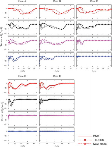
The corresponding model parameters are given as:

(11g)

(11h)

(11i)

The model parameter has been introduced in order to capture the augmentation of negative contribution of in the near-wall region, whereas is responsible for changing the sign of the model prediction and makes sure this change in sign becomes active at . However, vanishes away from the wall (i.e., ) and thus Eq. (11f) becomes identical to the T4D2CS model, i.e., Eq. (11e), which can be substantiated from Figure 10, where the predictions of Eq. (11f) are also shown. It can be seen from Figure 10 that the model given by Eq. (11f) adequately predicts the augmentation of the magnitude of negative contribution of in the near-wall region and also captures a slightly positive value of in the region given by . Thus, Eq. (11f) can be used for modeling both close to and away from the wall.

Conclusions

The SDR transport and its modeling in the context of RANS have been analyzed for head-on quenching of turbulent premixed flame by an inert isothermal wall based on 3D simple chemistry DNS data. It has been found that an increase in leads to an increase in the magnitudes of the unclosed terms of the SDR transport equation. For all cases the terms arising from density variation, scalar-turbulence interaction, reaction rate gradient, molecular diffusivity gradient, and molecular dissipation, i.e., , and , remain the leading order contributors to the SDR transport away from the wall, and the turbulent transport and molecular diffusion terms remain negligible in comparison to the aforementioned leading order terms. A rough equilibrium between ( and has been observed away from the wall before the quenching is initiated, but this equilibrium is not maintained at the vicinity of the wall during flame quenching. The performances of previously proposed models for , and have been assessed with respect to the corresponding quantities extracted from DNS data. It has been found that the aforementioned models do not adequately predict the near-wall behavior of the unclosed terms of the SDR transport equation. The models, which exhibit the most promising performance away from the wall, have been modified to account for the near-wall behavior in such a manner that they asymptotically approach the existing model expressions away from the wall. Although the functional form of the modeling parameters have been proposed so that they follow the asymptotic behavior in terms of , and , it is likely that they will need to be modified when datasets with a larger range of with detailed chemistry will be explored. It is worth noting that several previous DNS analyses on flame-wall interaction used a simple chemical mechanism (Alshaalan and Rutland, 1998, 2002; Bruneaux et al., 1996, 1997; Poinsot et al., 1993) and the same approach has been followed here. Moreover, all existing SDR transport closures have been proposed based on simple chemistry DNS data (Chakraborty et al., 2011; Chakraborty and Swaminathan, 2007a, 2007b, 2010, 2013; Kolla et al., 2009; Mura et al., 2008, 2009; Swaminathan and Bray, 2005). Since statistical behaviors of have been adequately captured by single-step chemistry [see Chakraborty and Klein (2008) and Chakraborty et al. (2008b, 2013) for scalar gradient statistics based on both simple and detailed chemistry DNS data], it can be expected that the findings will at least be qualitatively valid in the context of detailed chemistry and transport. However, a different wall boundary condition (e.g., adiabatic wall boundary condition) may lead to the modification of some of the wall corrections proposed here, but this analysis is beyond the scope of this article. Moreover, Lewis number may have some influence on the modeling of SDR transport but the qualitative nature of the present findings is unlikely to be modified (Chakraborty and Swaminathan, 2010). This necessitates comprehensive experimental and DNS-based validations at high values of for accurate estimation of the model parameters. Furthermore, the proposed models need to be implemented in actual RANS simulations to assess their predictive capabilities. Some of the aforementioned issues will form the foundation of future analyses.

Acknowledgment

The authors are grateful to N8/ARCHER for computational support.

Funding

The authors gratefully acknowledge the School of Mechanical and Systems Engineering of Newcastle University for the financial support.

Additional information

Funding

The authors gratefully acknowledge the School of Mechanical and Systems Engineering of Newcastle University for the financial support.

References

- Ahmed, I., and Swaminathan N. 2014. Simulation of turbulent explosion of hydrogen-air mixtures. J. Hydrogen Energy, 39(17), 9562–9572.
- Alshaalan, T.M., and Rutland, C.J. 1998. Turbulence, scalar transport, and reaction rates in flame-wall interaction. Proc. Combust. Inst., 27, 793.
- Alshaalan, T.M., and Rutland, C.J. 2002. Wall heat flux in turbulent premixed reacting flow. Combust. Sci. Technol., 174, 135.
- Batchelor, G.K., and Townsend, A.A. 1948. Decay of turbulence in final period. Proc. R. Soc. London, A194, 527.
- Borghi, R. 1990. Turbulent premixed combustion: Further discussion on the scales of fluctuations. Combust. Flame, 80, 304.
- Bray, K.N.C. 1980. Turbulent flows with premixed reactants. In P.A. Libby and F.A. Williams (Eds.), Turbulent Reacting Flows, Springer Verlag, Berlin, Heidelburg, New York, pp. 115–183.
- Bray, K.N.C., Libby, P.A., and Moss, J.B. 1985. Unified modelling approach for premixed turbulent combustion—Part I: General formulation. Combust. Flame, 61, 87.
- Bruneaux, G., Akselvoll, K., Poinsot, T., and Ferziger, J.H. 1996. Flame-wall interaction simulations in a turbulent channel flow. Combust. Flame, 107, 27.
- Bruneaux, G., Poinsot, T., and Ferziger, J.H. 1997. Premixed flame-wall interaction in a turbulent channel flow: Budget for the flame surface density evolution equation and modelling. J. Fluid. Mech., 349, 191.
- Butz, D., Gao, Y., Kempf, A.M., and Chakraborty, N. 2015. Large eddy simulations of a turbulent premixed swirl flame using an algebraic scalar dissipation rate closure. Combust. Flame, 162, 3180.
- Chakraborty, N., and Cant, R.S. 2009. Effects of Lewis number on scalar transport in turbulent premixed flames. Phys. Fluids, 21, 035110.
- Chakraborty, N., and Cant, R.S. 2011. Effects of Lewis number on flame surface density transport in turbulent premixed combustion. Combust. Flame, 158, 1768.
- Chakraborty, N., Champion, M., Mura, A., and Swaminathan, N. 2011. Scalar dissipation rate approach to reaction rate closure. In N. Swaminathan and K.N.C. Bray (Eds.), Turbulent Premixed Flame, 1st ed., Cambridge University Press, Cambridge, UK, pp. 76–102.
- Chakraborty, N., Hawkes, E.R., Chen, J.H., and Cant, R.S. 2008b. Effects of strain rate and curvature on surface density function transport in turbulent premixed CH4-air and H2-air flames: A comparative study. Combust. Flame, 154, 259.
- Chakraborty, N., and Klein, M. 2008. Influence of Lewis number on the surface density function transport in the thin reaction zones regime for turbulent premixed flames. Phys. Fluids, 20, 065102.
- Chakraborty, N., Klein, M., and Swaminathan, N. 2009. Effects of Lewis number on reactive scalar gradient alignment with local strain rate in turbulent premixed flames. Proc. Combust. Inst., 32, 1409.
- Chakraborty, N., Kolla, H., Sankaran, R., Hawkes, E.R., Chen, J.H., and Swaminathan, N. 2013. Determination of three-dimensional quantities related to scalar dissipation rate and its transport from two-dimensional measurements: Direct numerical simulation based validation. Proc. Combust. Inst., 34, 1151.
- Chakraborty, N., Rogerson, J.W., and Swaminathan, N. 2008a. A-priori assessment of closures for scalar dissipation rate transport in turbulent premixed flames using direct numerical simulation. Phys. Fluids, 20, 045106.
- Chakraborty, N., Rogerson, J., and Swaminathan, N. 2010. The scalar gradient alignment statistics of flame kernels and its modelling implications for turbulent premixed combustion. Flow Turbul. Combust., 85, 25.
- Chakraborty, N., and Swaminathan, N. 2007a. Influence of Damköhler number on turbulence–scalar interaction in premixed flames, Part I: Physical insight. Phys. Fluids, 19, 045103.
- Chakraborty, N., and Swaminathan, N. 2007b. Influence of Damköhler number on turbulence–scalar interaction in premixed flames, Part II: Model development. Phys. Fluids, 19, 045104.
- Chakraborty, N., and Swaminathan, N. 2010. Effects of Lewis number on scalar dissipation transport and its modelling implications for turbulent premixed combustion. Combust. Sci. Technol., 182, 1201.
- Chakraborty, N., and Swaminathan, N. 2011. Effects of Lewis number on scalar variance transport in premixed flames. Flow Turbul. Combust., 87, 261.
- Chakraborty, N., and Swaminathan, N. 2013. Effects of turbulent Reynolds number on the scalar dissipation rate transport in turbulent premixed flames in the context of Reynolds averaged Navier Stokes simulations. Combust. Sci. Technol., 185, 676.
- Chen, J.H., Choudhary, A., de Supinski, M., de Vries, B., Hawkes, E.R., Klasky, S., Liao, W.K., Ma, K.L., Mellor-Crummey, J., Podhorski, N., Sankaran, R., Shende, S., and Yoo, C.S. 2009. Terascale direct numerical simulations of turbulent combustion using S3D. Comput. Sci. Discovery, 2, 015001.
- Dabireau, F., Cuenot, B., Vermorel, O., and Poinsot, T. 2003. Interaction of flames of H2-O2 with inert walls. Combust. Flame, 135, 123.
- Dong, H.Q., Robin, V., Mura, A., and Champion, M. 2013. Analysis of algebraic closures of the mean scalar dissipation rate of the progress variable applied to stagnating turbulent flames. Flow Turbul. Combust., 90, 301.
- Dunstan, T., Minamoto, Y., Chakraborty, N., and Swaminathan, N. 2013. Scalar dissipation rate modelling for large eddy simulation of turbulent premixed flames. Proc. Combust. Inst., 34, 1193.
- Echekki, T., and Chen, J.H. 1999. Analysis of the contribution of curvature to premixed flame propagation. Combust. Flame, 118, 303.
- Gao, Y., Chakraborty, N., Dunstan, T.D., and Swaminathan, N. 2015c. Assessment of Reynolds averaged Navier Stokes modelling of scalar dissipation rate transport in turbulent oblique premixed flames. Combust. Sci. Technol., 187(10), 1584.
- Gao, Y., Chakraborty, N., and Swaminathan, N. 2014. Algebraic closure of scalar dissipation rate for large eddy simulations of turbulent premixed combustion. Combust. Sci. Technol., 186, 1309.
- Gao, Y., Chakraborty, N., and Swaminathan, N. 2015a. Dynamic closure of scalar dissipation rate for large eddy simulations of turbulent premixed combustion: A direct numerical simulations analysis. Flow Turbul. Combust, 95, 775.
- Gao, Y., Chakraborty, N., and Swaminathan, N. 2015b. Scalar dissipation rate transport and its modelling for large eddy simulations of turbulent premixed combustion. Combust. Sci. Technol., 187(3), 362.
- Gruber, A., Chen, J.H., Valiev, D., and Law, C.K. 2012. Direct numerical simulation of premixed flame boundary layer flashback in turbulent channel flow. J. Fluid Mech., 709, 516.
- Gruber, A., Sankaran, R., Hawkes, E.R., and Chen, J.H. 2010. Turbulent flame-wall interaction: A direct numerical simulation study. J. Fluid. Mech., 658, 5.
- Huang, W.M., Vosen, S.R., and Greif, R. 1986. Heat transfer during laminar flame quenching. Proc. Combust. Inst., 21, 1853.
- Jarosinsky, J. 1986. A survey of recent studies on flame extinction. Combust. Sci. Technol., 12, 81.
- Jenkins, K.W., and Cant, R.S. 1999. Direct numerical simulation of turbulent flame kernel. In Recent Advances in DNS and LES, D. Knight and L. Sakell (Eds.), Springer, pp. 191–202.
- Kolla, H., Rogerson, J.W., Chakraborty, N., and Swaminathan, N. 2009. Scalar dissipation rate modeling and its validation. Combust. Sci. Technol., 181, 518.
- Kolla, H., and Swaminathan, N. 2010. Strained flamelets for turbulent premixed flames, II: Laboratory flame results. Combust. Flame, 157, 1274.
- Lai, J., and Chakraborty, N. 2016. Effects of Lewis number on head on quenching of turbulent premixed flame: A direct numerical simulation analysis. Flow Turbul. Combust, 96, 279.
- Langella, I., Swaminathan, N., Gao, Y., and Chakraborty, N. 2015. Assessment of dynamic closure for premixed combustion large eddy simulation. Combust. Theor. Model, 19, 628.
- Ma, T., Gao, Y., Kempf, A.M., and Chakraborty, N. 2014. Validation and implementation of algebraic LES modelling of scalar dissipation rate for reaction rate closure in turbulent premixed combustion. Combust. Flame, 161, 3134.
- Mantel, T., and Borghi, R. 1994. A new model of premixed wrinkled flame propagation based on a scalar dissipation equation. Combust. Flame, 96, 443.
- Mura, A., and Borghi, R. 2003. Towards an extended scalar dissipation equation for turbulent premixed combustion. Combust. Flame, 133, 193.
- Mura, A., Robin, V., Champion, M., and Hasegawa, T. 2009. Small-scale feactures of velocity and scalar fields of turbulent premixed flames. Flow Turbul. Combust., 82, 339.
- Mura, A., Tsuboi, K., and Hasegawa, T. 2008. Modelling of the correlation between velocity and reactive scalar gradeints in turbulent premixed flames based on DNS data. Combust. Theor. Model., 12, 671.
- Peters, N. 2000. Turbulent Combustion, Cambridge University Press, Cambridge, UK.
- Peters, N., Terhoeven, P., Chen, J.H., and Echekki, T. 1998. Statistics of flame displacement speeds from computations of 2-D unsteady methane-air flames. Proc. Combust. Inst., 27, 833.
- Poinsot, T.J., Haworth, D.C., and Bruneaux, G. 1993. Direct simulation and modelling of flame-wall interaction for premixed turbulent combustion. Combust. Flame, 95, 118.
- Robin, V., Guilbert, N., Mura, A., and Champion, M. 2010. Turbulent combustion modeling of mixtures with inhomogeneous equivalence ratio. Application to a flame stabilized by the sudden expansion of a 2-D channel. C.R. Mec., 338, 40.
- Rogallo, R.S. 1981. Numerical experiments in homogeneous turbulence. NASA Technical Memorandum 81315. NASA Ames Research Center, Moffett Field, CA.
- Sadasivuni, S., Bulat, G., Senderson, V., and Swaminathan, N. 2012. Application of scalar dissipation rate model to Siemens DLE combustors. Paper No. GT2012-68483. Presented at the ASME Turbo Expo 2012, Copenhagen, Denmark, June 11–15.
- Swaminathan, N., and Bray, K.N.C. 2005. Effect of dilatation on scalar dissipation in turbulent premixed flames. Combust. Flame, 143, 549.
- Swaminathan, N., and Grout, R.G. 2006. Interaction of turbulence and scalar fields in premixed flames. Phys. Fluids, 18, 045102.
- Tennekes, H., and Lumley, J.L. 1972. A First Course in Turbulence, MIT Press, Cambridge, MA.
- Veynante, D., Trouvé, A., Bray, K.N.C., and Mantel, T. 1997. Gradient and countergradient turbulent scalar transport in turbulent premixed flames. J. Fluid Mech., 332, 263.
- Vosen, S.R., Greif, R., and Westbrook, C. 1984. Unsteady heat transfer in laminar flame quenching. Proc. Combust. Inst., 20, 76.
- Wray, A.A. 1990. Minimal storage time advancement schemes for spectral methods. NASA Ames Research Center, Moffett Field, CA.