Large-Eddy Simulation of Premixed Combustion in the Corrugated-Flamelet Regime

ABSTRACT

Large-eddy simulation (LES) is applied to a fuel-lean turbulent propane-air Bunsen flame in the corrugated-flamelet regime. The subgrid-scale (SGS) modeling includes a previously developed treatment of the total enthalpy along with three different SGS velocity, , models. In addressing the filtered reaction rate, a presumed probability density function (PDF) approach is employed for the reaction-progress variable, closed by a transport equation for its SGS variance. The statistics obtained using the three models are in good agreement with the measurements and do not differ significantly from each other for first-order moments suggesting that commonly used SGS modeling may be adequate to get the mean velocities and reaction progress variable. However, all three SGS velocity models fail to reflect a measured bimodality of the PDF of the radial component of the velocity in the central portion of the flame. This emphasizes a need for further development of models required at the reaction rate closure level for practical LES of combustion in the corrugated-flamelet regime.

KEYWORDS:

• Flamelets
• Large eddy simulation (LES)
• Premixed combustion
• Subgrid scale (SGS) velocity

Introduction

Lean premixed combustion is attractive for practical combustion devices because of its potential to deliver high efficiency and low emissions simultaneously. The sensitivity of lean premixed flames to fluctuations in fluid-dynamic and thermochemical conditions of the reactant mixture, however, causes numerical modeling of such combustion processes to be challenging. Many different modeling avenues have been developed; a summary of the approaches to large-eddy simulation (LES) of premixed combustion is given in Poinsot and Veynante (2005), Pitsch (2006), Gicquel et al., (2012), Swaminathan and Bray (2011), and Cant (2011). These approaches can be broadly categorized into flamelet and non-flamelet approaches, the former being selected here for the present investigation. Flamelet approach can be further subdivided into geometrical and statistical approaches, with the G-equation and flame-surface-density-based methods belonging to the geometrical category and presumed probability density function (PDF) methods to the statistical category. Flamelet models based on artificial thickening or filtering of laminar flame are also possible (Duwig, 2007; Nguyen et al., 2010; Wang et al., 2011). The present contribution falls within PDF methods, working with a presumed PDF for a reaction-progress variable.

Premixed combustion occurs in different regimes, depending on the competing effects of turbulence and finite-rate chemistry. The flame structures in different regimes differ significantly, ranging from wrinkled flamelets at low turbulence intensities to distributed reaction zones at high intensities (Peters, 2000). The corrugated-flamelet regime lies adjacent to the wrinkled-flamelet regime and is separated from regimes at higher turbulence intensities by the thin-reaction-zone regime. The latter is typical of piloted flames, having high Reynolds numbers and experiencing strong turbulence resulting predominantly from shear-production mechanisms, representative of most practical applications. For this reason, many LES studies aimed at predicting experimental observations have been focused on the thin-reaction-zones regime combustion (Colin et al., 2000; De and Acharya, 2009; Gubba et al., 2012; Langella et al., 2015; Wang et al., 2012) and a direct numerical simulation (DNS) with tabulated chemistry approach has been also been attempted for an experimental configuration (Moureau et al., 2011). There is also interest, however, in the corrugated-flamelet regime, in which, just as in the thin-reaction-zones regime, experimental Reynolds numbers are too large for DNS to be feasible, and for which the heat-release effects of the flames on the turbulence may be proportionally greater as a consequence of the lower incoming turbulence levels.

As a continuation of a series of experiments by Furukawa and co-workers (Furukawa et al., 2002; Furukawa and Williams, 2003; Furukawa et al., 2013a, 2013b), recently, Furukawa et al. (2016) reported measured statistics of gas velocities, with reaction-progress-variable fields deduced therefrom in a non-piloted lean propane-air premixed Bunsen flame in an open environment. This is one of four flames in the corrugated-flamelet regime that they investigated, and they suggested that it would be of interest to pursue numerical modeling of the experimental results. Because of the aforementioned importance of fuel-lean combustion, the present work was performed with the aim of shedding light on the structure of this flame. This provides a good opportunity to gather insight into the capabilities and limitations of statistical flamelet models for subgrid-scale (SGS) combustion in LES of this flame. Since the shear-produced turbulence does not affect this flame, as one shall see in the results section, the turbulence level experienced by the flame results mainly from flame-intermittency and thermal-expansion effects. These are SGS phenomena in a practical LES, and thus they would affect the SGS velocity that needs to be modeled. It may be debatable whether one needs to include dilatation effect in this velocity modeling or not as propositions have been made in the past to exclude this effect in general (Colin et al., 2000). Three SGS velocity models treating the thermal-expansion effects differently are considered to assess their influence on the premixed combustion from both physical and numerical viewpoints.

This article is organized as follows. The experimental flame is described next in the next section. Following that the numerical model including the SGS combustion and velocity closures with the numerical procedures and boundary conditions are discussed. Results are presented and discussed in section the next, and concluding remarks are made in the final section.

Experiment

Figure 1 shows a direct photograph and a schematic diagram of the flame considered here, a propane-air flame having an equivalence ratio of . Calculations with the PREMIX code (Kee et al., 1985) and complex chemical-kinetic schemes (Sung et al., 1998; UC San Diego, 2014) produce a laminar flame speed of and a laminar-flame thermal thickness of . The reactant mixture issues from a pipe of diameter and spreads into an open environment, as shown schematically in Figure 1b. The bulk mean velocity based on the mass flow rate at cold conditions is . The shear layer present at the interface between jet and surrounding air encloses the flame as sketched in the figure, and this flame configuration is quite different from piloted turbulent premixed flames, where the flame resides inside the shear layer between reactant and pilot streams. Since the flame is not in the shear layer for this configuration, the turbulence experienced by the flame comes from the inlet initially produced by the fully developed turbulent pipe flow but modified by thermal-expansion effects and flame-front intermittency. In addition, the turbulence produced by the shear through the Kelvin–Helmoltz instability is not expected to affect the flame, as will be seen later.

Figure 1. A direct photograph (a) and a schematic (b) of the lean propane-air flame of Furukawa et al. (2016).

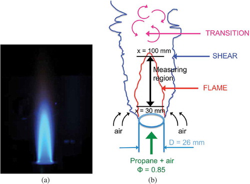
A 3D LDV (laser Doppler velocimetry) system having a spherical resolution volume of about 0.2 mm diameter was used to measure three components of velocity, from which various characteristics of the flame were deduced. Measurements along the centerline were taken from to 110 mm and along the radius for at given height, h, ranging from 30 mm to 90 mm. These measurement regions, indicated in Figure 1b, did not include the shear layer or region where the shear layer interacts with the core of the jet (marked as “Transition” in Figure 1b). In other words, the measurements were focused in regions where shear-generated turbulence effects are weak. This experiment offers a good challenge for combustion modeling because the turbulence induced by the flame intermittency and the turbulence-flame interaction is important in these flames, affecting the required physics of submodels.

Numerical model

Governing equations

The Favre-filtered conservation equations for mass, momentum, and total enthalpy are solved along with other equations required for premixed combustion. These additional equations include filtered progress variable and its SGS variance, to be discussed in the next subsection. The instantaneous progress variable, c, is defined as , where is the fuel mass fraction in the unburned mixture and c takes a value of 0 and 1 in the fresh and burned mixtures, respectively. The subgrid stresses are closed using a localized dynamic Smagorinsky model (Germano et al., 1991; Lilly, 1992) and the SGS scalar fluxes are computed using a gradient hypothesis with a dynamic Schmidt number approach (Lilly, 1992). The modeling constant in the localized dynamic Smagorinsky model used here decreases to zero in laminar regions making this model suitable also for low-turbulence regions investigated here. However, other choices like Vreman (Vreman, 2004) or static Sigma (Nicoud et al., 2011) models are possible and these models are expected to give improvements only close to walls or in transitional regions (Kemenov et al., 2012; Rieth et al., 2014; Vreman, 2004) (not relevant for this study). Furthermore, these models involve additional model constants (thus their tuning) and so they are not considered for this study. Also, the SGS scalar fluxes are treated using gradient transport hypothesis as in many earlier LES and the influence of counter-gradient transport for these fluxes, which may exist for most part of the filtered flame under the conditions investigated here, is of interest for a future study. However, adequacy of the gradient hypothesis can be investigated using the experimental comparisons shown in later sections of this article.

The transport equation for the filtered total enthalpy, , is:

1

where is the thermal diffusivity. The Favre-filtered temperature, , is computed as , where is the enthalpy of formation for the mixture and is the specific heat at constant pressure for the mixture, which depends on temperature as described by Ruan et al. (2014), where further details may be found. The mixture density is computed from the state equation, , where is the filtered pressure, is the Favre-filtered molecular weight of the mixture and is the universal gas constant.

In the code, in general, the values of , , and are computed on the basis of the formula:

2

where refers to any one of the three quantities above, is its value in air, and is its value in the reacting mixture. This mixing rule is used to include the dilution of burned mixture with the entrained air. A transport equation is used to compute the Favre-filtered passive marker, , and this equation is:

3

where is the diffusivity of . The values of are computed from laminar-flamelet values using an equation similar to Eq. (4) to be discussed later. The flamelet values are obtained by computing unstrained planar laminar flames using the PREMIX code (Kee et al., 1985) and complex chemical-kinetic schemes for propane-air combustion. Two mechanisms (Sung et al., 1998; UC San Diego, 2014) were considered but no substantial differences in the laminar-flame structures, speed, or thickness were observed.

Combustion closure

The filtered reaction rate and its related terms in the SGS variance equation are closed using an unstrained flamelet approach. The filtered reaction rate is modeled as:

4

where and is the density weighted subgrid PDF with as the sample space variable for . The flamelet reaction rate is , which is obtained from the freely propagating unstrained planar laminar flame for a given thermochemical

If this fiugure was previously printed in another publication please obtain permission to reprint from the original publisher and provide documentation.

condition. The subgrid PDF is modeled using the beta function, which is expressed as:

5

The parameters a and b are related to the filtered progress variable, , and SGS variance, , through:

6

The choice of a beta-PDF is not uncommon for LES of premixed combustion and has been employed with good results in many past studies, see, for example, Landenfeld et al. (2002), Domingo et al. (2005), Vreman et al. (2009), Lecocq et al. (2010, 2011), Moureau et al. (2011), Nambulli et al. (2014), and Langella and Swaminathan (2015). Fiorina et al. (2015) remarked that the beta-PDF is not relevant when the SGS flame wrinkling is completely resolved. When this wrinkling is fully resolved (which is a DNS) then the SGS PDF would be a delta function. One would need a very fine grid to resolve the SGS wrinkling, which is not the objective in this article, where the aim is to keep the LES practical. Moreover, the beta-PDF automatically captures the bimodal behavior due to flame intermittency when the SGS variance, which is high due to intermittency, is well predicted as one shall see next. However, other choices of PDF are possible.

The values of and are obtained by solving their transport equations. The progress variable equation is:

7

where is the molecular diffusivity of c. The transport equation for is written as:

8

where and are the SGS viscosity and Schmidt number. The third term of Eq. (8) related to chemical reaction is closed by using:

9

which is consistent with the closure in Eq. (4). The subgrid dissipation rate (SDR) is defined from the equation and is closed using an algebraic model (Dunstan et al., 2013):

10

This model for the SDR has been used in conjunction with an algebraic reaction-rate closure for LES of piloted turbulent Bunsen flames (Langella et al., 2015). A similar model with corrections for nonunity Lewis numbers has also been studied using DNS (Gao et al., 2014a, 2014b) and LES (Butz et al., 2015; Ma et al., 2014). The factor in Eq. (10), defined as , with and , ensures that when . The filter width, , is assumed to be following common practice, where is the volume of cell . The subgrid Damköhler number is , where is the chemical time scale and is the SGS flow time scale, and being the SGS kinetic energy and dissipation rate, respectively. These two SGS quantities are related to and the SGS velocity , which requires modeling. The heat-release parameter is , where is the adiabatic flame temperature and is the reactant temperature. The term describes the effects of flame-front curvature induced by turbulence, chemical reaction, and molecular dissipation. The scale-dependent parameter has previously been obtained dynamically (Gao et al., 2015; Langella and Swaminathan, 2015; Langella et al., 2015), but that approach cannot be used for the flame investigated here because of the low turbulence level. A dynamic procedure usually invokes scale-similarity assumption, which holds if the energy of a fluctuating reacting scalar decreases monotonically around the scale of interest, which is the flame scale. If the turbulence level is low then the energy at SGS level may be significantly larger than that at the smallest resolved scale. Then, the dynamic procedure becomes ill-posed as noted by Charlette et al. (2002) for a dynamic power-law formulation. This issue is different to dynamic formulation for SGS stresses, like the dynamic Smagorinsky model, where the turbulent kinetic energy cascade to the small scales implies that the energy level between two subsequent scales is always similar. The dynamic formulation for may lead to its singularity [the denominator of Eq. (4) in Langella et al. (2015) may approach zero], which is unphysical. This was verified through preliminary simulations and for these reasons a static value of is used, as detailed in the first subsection under “Results.”

The terms () and arise from fluctuating dilatation and strain rate resulting from competing effects of turbulence and heat release, respectively, and they are all influenced by SGS turbulence. The parameters describing the influences of thermochemical and turbulence processes and their interplay are , , and , where the SGS Karlovitz number is (Dunstan et al., 2013). The basis for these functional forms is discussed in detail elsewhere (Chakraborty and Swaminathan, 2007; Dunstan et al., 2013; Kolla et al., 2009).

The SGS velocity, , is modeled in three different ways:

1. A model based on SGS stress-related closure proposed by Lilly (1967), given by:

   11

   where is the turbulent viscosity modeled using a localized dynamic Smagorinsky model. The model constant is .

2. A second model based on scale-similarity for velocity is (Pope, 2000):

   12

   where is the velocity vector field obtained using a Gaussian test filter of width . Different estimates for have been given in the literature (Bardina et al., 1980; Colucci et al., 1998; Métais and Lesieur, 1992), and its dynamic evaluation is possible (Cook, 1997), but that requires an estimate for the integral length scale, which is not easy. Also, the turbulence level is low for the experimental flame. For this reason the value , which is comparable to the previous estimates, is used here.

3. Colin et al. (2000) derived another model by expanding Eq. (12) in a Taylor series up to second order and then applying the curl operator to exclude dilatation effects. The resulting expression is:

   13

   where is a typical value suggested by Colin et al. (2000).

One could also use a transport equation for SGS kinetic energy, , to compute both SGS stresses in the momentum equation and to evaluate the SGS velocity through . This transport equation involves pressure correlation terms, which are important for combustion in corrugated-flamelet regime. These terms need modeling and no satisfactory model for LES of premixed combustion is available in the literature. For these reasons, this transport equation is not employed for this study.

Numerical method and boundary conditions

The above conservation and modeled equations are solved with a finite-volume code, PRECISE-MB (Anand et al., 1999). The spatial derivatives are discretized by a second-order central-differencing scheme for all variables except the progress variable and its variance, which are discretized using a nonoscillatory bounded HLPA (hybrid linear/parabolic approximation) scheme (Zhu, 1991; Zhu and Rodi, 1991). The time advancement is performed using a second-order scheme with a constant time step so that the CFL number is smaller than 0.3 in the entire computational domain. The velocity-pressure coupling is achieved by using the SIMPLEC algorithm (Doormaal and Raithby, 1984).

The cylindrical computational domain with is discretized on a nonuniform grid having cells in the radial and axial directions, respectively, with 44 cells for the jet diameter, , and 80 cells in the azimuthal direction. This grid results in 5.4M cells in total for the chosen computational volume. The filter size, based on the numerical cell volume, has a minimum width of (0.52 mm) close to the jet exit. Another refined grid having about 23M cells, obtained by increasing the number of cells by about 60% in all three directions, is used to test grid dependency of the flame statistics.

The progress variable is assigned to be 0 and 1 for the reactant jet and entrainment inlet boundaries, respectively. A small velocity of 0.1 m/s and a temperature of 298 K are assigned for the entrained air at the respective inlet boundary. Slip-flow and zero-gradient conditions are assigned on the lateral boundaries for velocity and scalars, respectively. A zero-gradient condition is applied at the outlet for all variables but pressure, which is assigned to be atmospheric.

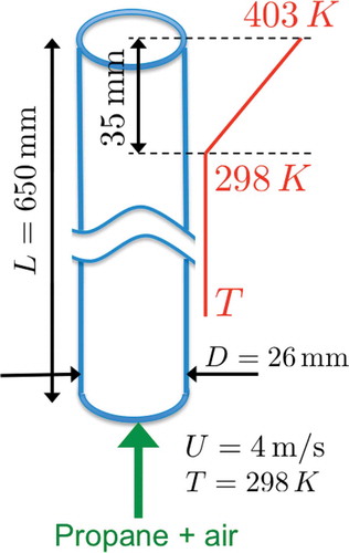
The cold-flow velocity measurements had provided an exit velocity profile with a maximum velocity on the centerline of (Furukawa et al., 2016). This value, however, is inconsistent with the measured and calculated centerline value of 5.5 m/s at about one exit-diameter distance from the jet exit, implying a strong acceleration over this distance if it were 4.5 m/s at the jet exit. This observation prompted further measurements of jet tube-wall temperature since wall heating of the reactant mixture inside the tube when the flame is present could cause the exit velocity to increase. To capture these influences correctly, a preliminary RANS simulation using Fluent code and model was performed for the computational domain and conditions illustrated in Figure 2. This cylindrical domain is discretized using cells in radial and axial directions, respectively. In terms of wall units, the first cell close to the wall at the pipe exit has , where is the radial coordinate, is the kinematic viscosity of the flow, and is the shear velocity, being the shear stress at the wall, and these quantities are evaluated a posteriori. Thus, the boundary layer is not resolved and the wall-enhancement treatment in Fluent has been used to account for the proper resolution of the flow near the wall. The measured mass flow rate of the propane-air mixture at 298 K is specified at the inlet with flat profiles. A linear temperature profile in the vertical direction along the wall, as shown in the figure, was specified near the exit, based on experimental wall-temperature estimates. This linear profile gives a temperature gradient of about 3 K/mm along the wall.

Figure 2. Numerical domain for the preliminary RANS.

The radial variations of axial velocity and temperature at the jet exit obtained from this RANS calculation are shown in Figures 3a and 3b, respectively. The temperature at the jet exit is nonuniform and accelerates the flow. The centerline value of axial velocity was calculated to be about 5.4 m/s, which is close to 5.5 m/s observed in the experiment at from the jet exit. The axial velocity variation in the cold condition shown in Figure 3a depicts the flow acceleration when the wall temperature varies axially. These computed profiles for nonisothermal flow were specified as boundary conditions for the LES.

Figure 3. Axial velocity (a), temperature (b), and axial velocity rms (c) profiles at the jet exit, computed using RANS. The dashed line is for isothermal case.

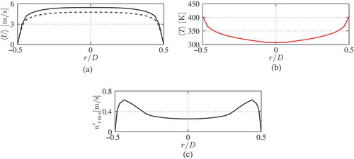
Although the rms value of 0.22 m/s, reported by Furukawa et al. (2016), is low at the jet exit, it is important to include this because the flame experiences only this turbulence and does not see the shear-generated turbulence as noted earlier. A synthetic turbulence having similar characteristics as in the experiment, therefore, was generated using the digital-filter technique (Klein et al., 2002) and was added to the velocity shown in Figure 3a for the jet exit. The variations of rms velocity in three directions are imposed using the turbulent kinetic energy obtained from the RANS computation. The value in the axial direction is taken to be twice that in the other two directions. This is acceptable because the centerline value in the axial direction, , is close to the measured value of 0.22 m/s. This gives , which is slightly smaller than the measured value of for the cold flow.

The radial variation of at the jet exit is shown in Figure 3c. The measured longitudinal integral length scale of and the transversal length scales of are used. The scales are taken to be uniform as required by the digital filter technique (Klein et al., 2002). The assigned turbulence may thus have some uncertainty and so a sensitivity analysis has been performed by varying the inlet rms values. An increase of of the rms produces an almost decrease in flame length, while a zero inlet rms results in a flame length almost longer than the measured value and also an increased flame ‘flapping’ leading to the PDFs to exhibit skewness when this artificial inlet condition is applied. This analysis enlightens a strong sensitivity of the flame to the inlet turbulence as anticipated. The uncertainty at the inlet will be removed to some extent in this study by carefully selecting the modeling parameter to yield the measured flame length (see the next section).

The grid size was also increased by a factor of 1.6 in all directions, resulting in 23M cells for the same computational volume as noted earlier to test grid sensitivity. The CFL number was kept below 0.3 everywhere in the domain by using constant time steps of and , respectively, for the 23M and 5.4M grids. The LES are run for of real time using 208 cores for 23M and 32 cores for 5.4M grids, of which the latter half is used for collecting statistics. These simulations took about 72 h on a wall clock using 2.60 GHz eight-core Sandy Bridge E5-2670 processors of the Darwin cluster at Cambridge University.

Results

Role of SGS velocity modeling

The SGS velocity will be influenced by dilatation resulting from combustion, whence values obtained from Eqs. (11) to (13) can differ, since these models presume the role of the dilatation differently. Any difference in gives a different according to Eq. (10), which influences . This can influence the filtered reaction rate [see Eqs. (4) to (6)], which, in turn, can affect the . Thus, the combustion model employed here has two-way coupling between the flame and the turbulence.

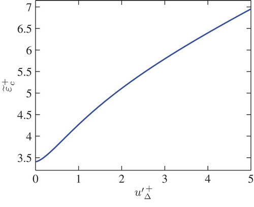
Figure 4 shows the sensitivity of the SDR (normalized by ) to (also normalized), while keeping other parameters in Eq. (10) to be constant, with , a representative value for the flame regions based on the grid used here. The quantity is taken to be unity for the purpose of this estimate. The variation is weakly nonlinear for the range shown, a 100% change in producing only about a 20% change in . This implies that the same variation could be obtained by changing by about 20%.

Figure 4. Variation of , with .

Since the incoming turbulence influences , any difference in its value obtained synthetically can also influence . The subgrid velocity can be written as with a constant and given by Eqs. (11) to (13) without their respective model constants. Because of the near linearity observed in Figure 4, Eq. (10) can be approximated as:

14

where and is to be found to minimize the error (for example, using gives a maximum error below 2% in the range ). This is not necessary because the objective here is to demonstrate that and models can be tuned simultaneously as discussed below, and Eq. (14) is not actually used for computation. From Eq. (14), the variation of dissipation rate can be expressed as . The variation of for is shown in Figure 4. From Eq. (14) one can define , which can be used instead of and because of the near linearity of with observed in Figure 4 over the range of expected for the confguration investigated in this study. The value of for the various models is chosen by matching the computed and measured flame lengths, estimated to be the location of the peak axial velocity from the jet exit along the centerline, to complete a comparative analysis. It is worth noting that such analysis would not be possible without considerable uncertainty for quantities with no experimental data. The above tuning was necessary to overcome the difficulty produced by the modeling constants of SGS velocity and SDR models, and to some extent that of the inlet turbulence, which affects directly the flame length as discussed in the last section. Alternatively, when dynamic modeling is not possible one might use values suggested by experiments or DNS data available in the literature [see Gao et al. (2014a) for analysis of using DNS data], which are, however, not universal. This was unnecessary in this study where experimental data is available, and some tuning is probably the best choice to minimize uncertainties for a meaningful comparative analysis.

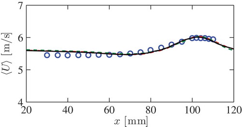
The values of obtained using the three models given in Eqs. (11) to (13), respectively, Lilly, Pope, and Colin et al. models, are shown in Table 1. The for Lilly model is larger than those for the other two models, suggesting that the SGS velocity estimated by it is also different as will be seen later. The computed axial velocity along the centerline is compared to the measured values in Figure 5 for the three models. Practically there is no difference among the computed values, which also agree well with measurements.

Table 1. Optimum values of found using the three SGS velocity models in Eqs. (11) to (13).

Model	Lilly (Eq. 11)	Pope (Eq. 12)	Colin et al. (Eq. 13)
	10.0	6.0	6.0

Figure 5. Comparison of measured (symbols) and computed axial velocity along the centerline; Lilly model, Eq. (11) (dashed line), Pope model, Eq. (12) (continuous line), and Colin et al. model, Eq. (13) (dash-dotted line).

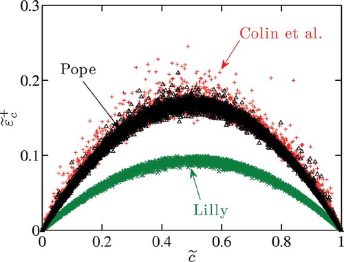
The variation of within the filtered flame is shown in Figure 6 for the three models. The values obtained from Pope, Eq. (12), and Lilly, Eq. (13), models for look similar, with the latter exhibiting more scatter. The greater scatter with larger values is due to the effects of intermittency of the interface between the reacted jet fluid and entrained air at locations closer to the jet exit. The SDR with Lilly model, Eq. (11), is smaller as a result of the higher value of . This can be also interpreted to mean that this model needs reduced dissipation to achieve the same flame length or that it overestimates when is used.

Figure 6. Scatter plot of normalized sub-grid SDR vs. progress variable, obtained using models Eq. (11) (Lilly), Eq. (12) (Pope), and Eq. (13) (Colin et al.) for .

Further insights can be obtained by studying the spatial variation of , which is the time-averaged ; typical variations are shown in Figures 7a and 7b for the mid-plane. Formally, this quantity is [see Eq. (14)], and the plots are normalized by the respective maximum values to force the variation from 0 to 1, facilitating comparisons, needed because of the differences in . A significantly larger value and wider region is seen for the shear layer in the model of Colin et al., compared with that of Pope, even in nonreacting regions. Although the model of Colin et al. in Eq. (13) is derived from that of Pope in Eq. (12) there is no guarantee that the SGS velocities predicted with these two models will be the same for nonreacting regions. The maximum values of given in the figure occur near the jet exit, and their values inside the shear layer at are 0.15 m/s, 0.3 m/s, and 1.19 m/s for Eqs. (11), (12), and (13), respectively. The peak value from Colin et al. model, Eq. (13), is nearly three times larger than that from the Pope model, Eq. (12) for nonreacting regions where similar values are expected.

Figure 7. Contours of in the mid-plane. The values of are 0.15 m/s, 0.80 m/s and 2.03 m/s, respectively, for Lilly, Pope, and Colin et al. models. Mid-plane contours of , where is the resolved turbulent kinetic energy, are shown in (c) in m/s.

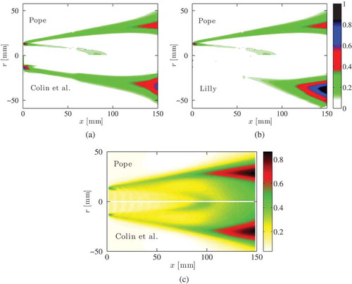
A second region having nonzero is seen in Figures 7a and 7b for Popes’ model, Eq. (12), resulting from flame-induced effects. This flame induced inside the flame brush is of a similar magnitude as that in the shear-layer region. The flame-induced SGS velocity is not visible for the model of Colin et al. because it is designed to exclude the dilatation effect. Nevertheless, the dimensional inside the flame brush obtained using Pope, Eq. (12), and Colin et al., (13) are both found to be about 0.2 m/s, masked for Eq. (13) by the very large value in the nonreacting region.

For Lilly model in Eq. (11), the value of in the region of the flame brush is about 0.02 m/s, an order of magnitude smaller than those of the other two models. Since the viscosity is computed dynamically, the dilatational part in Lilly model coming from the strain rate is masked by the fact that the Smagorinsky constant goes to zero in quasi-laminar regions. For the same reason approaches zero even in the shear region close to the jet exit, as seen in Figure 4b. It is worth noting that Lilly model was originally derived from the stresses without involving any dynamic constant. One can think of using this model with a sensible value for Smagorinsky constant (), which is known to work well when the turbulence level is sufficiently large. However, this approach is not followed here because it is less suited for quasi-laminar and inhomogeneous flows, and also would introduce additional uncertainty through the value for . The present study is only concerned to show that Lilly model is unsuitable for predicting effects of dilatation on the SGS velocity when dynamic Smagorinsky model is used for the SGS stresses. However, it would be of interest to investigate the influence of SGS stresses models on the SGS velocity, which is a case for a future study.

One can also compare the values with a turbulent velocity scale, , where is the resolved turbulent kinetic energy to assess the relative magnitude between SGS and resolved energy. This is shown in Figure 4c for Pope and Colin et al. models, which gives very similar predictions of . Lilly model also gives very similar predictions and thus is not shown. Using the data in Figure 4 it is easy to verify that a significant part of energy is at SGS scales (use Pope model). An estimation of the Pope’s criterion for turbulent kinetic energy, for regions of turbulence without combustion, is also possible and one can easily verify that this criterion is satisfied in the shear region for Lilly and Pope models but not Colin et al. model. However, this is irrelevant for the study here as the SGS velocity constants are scaled through the tuning of parameter as discussed at the beginning of this section. It is also worth noting that by definition is a residual kinetic energy and not residual turbulent kinetic energy.

The above analysis shows the potential of the various SGS velocity models considered here. The flame length in this analysis is tuned by selecting an appropriate value for , and the value of this parameter alters the amount of subgrid SDR in Eq. (14), which in turn alters the value of and thus . Since , the role of can be interpreted as that of controlling the magnitude of to maintain the correct value of . These comparisons of the models suggest that either the dilatation effect should be included in Eq. (13), or a different value for is required in that equation. Lilly model in Eq. (11) is not suitable for the present flame conditions because the dynamic viscosity used in that model approaches zero, causing the magnitude of to approach zero, becoming less than the fresh-mixture rms velocity fluctuation irrespective of flame-induced effects. It will be seen later, however, that none of these models address properly a dilatation-related subgrid velocity-fluctuation effect that is dominant in the center of the flame zone in the corrugated-flamelet regime.

Comparison of statistics

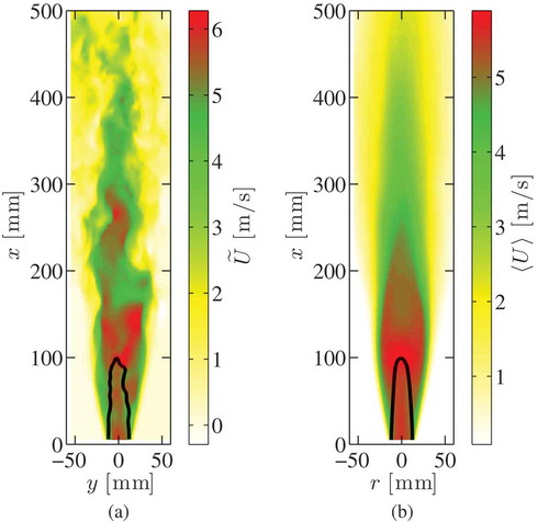
Figure 8 shows axial velocity contours, both instantaneous and time averaged, along with a contour of mean progress variable of . These contours indicate the positions of the shear layer and the flame, showing clearly that these two regions do not overlap. The jet becomes highly turbulent at , but the flame height is only about 100 mm. The acceleration through the flame tip is visible at , which is consistent with the experimental data, as seen in Figure 5.

Figure 8. Axial velocity instantaneous (a) and mean (b) contours, obtained using Eq. (12) for SGS velocity. Colors represent velocity in m/s. The Favre-filtered and mean progress variable isolines, and , are also shown (black line).

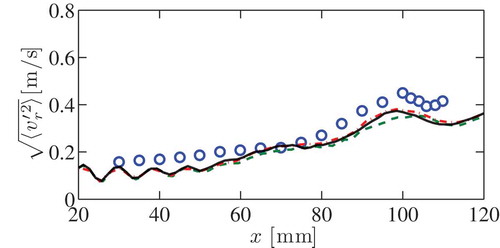
The computed rms of radial velocity fluctuation along the centerline is compared with the experimental data in Figure 9 for the three SGS velocity models. The values shown here are only the resolved parts, found to be insensitive to the model selected. The computed values are seen to agree reasonably with the experimental data. Some underestimate close to the jet exit arise from the uncertainties in the inlet turbulence. There is also some underestimate in the flame region and the reason for which will become clear in the next section.

Figure 9. Comparison of measured and computed centerline variation of radial rms velocity. Lilly model, Eq. (11) (dashed line), Pope model, Eq. (12) (continuous line), and Colin et al. model, Eq. (13) (dash-dotted line).

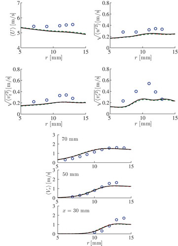
The radial variations of computed mean and rms velocities are compared with the experimental results in Figure 10. These statistics also are insensitive to the model, and , , and agree reasonably well with the experimental data. Some underprediction is seen in the mean (the maximum error being less than for axial velocity) and especially in the rms radial velocities close to the jet exit and for , i.e., in the flame region. This underprediction is related to the dilatation effects and a bimodal radial velocity PDF, which is discussed in detail in the next section. The mean velocities are predicted reasonably well also in nonreacting regions surrounding the flame, however, the rms values are underpredicted. The reasons for this might be related to the influences of dilatation effects.

Figure 10. Radial variations of mean and rms velocities. The axial mean and all three rms components are shown at an axial position 50 mm above the burner exit. Lilly model, Eq. (11) (dashed line), Pope model, Eq. (12) (continuous line), and Colin et al. model, Eq. (13) (dash-dotted line).

Reynolds- and Favre-averaged progress-variable statistics were also extracted from the experiments by deducing the progress variable from bimodal velocity data (Furukawa et al., 2016). This approach could not be tested by the LES because that broadens the flame at least to a size of . The transported propane-based progress variable is used here. The calculated radial variations of the Favre-averaged progress variable are compared with those from the experiment in Figure 11, where the solid curve corresponds to Pope model, Eq. (12), and the dashed curves, close to them, to Lilly and Colin et al. models, Eqs. (11) and (13). Error bars are shown for the experimental data at , and similar errors are expected for other heights. All SGS velocity models predict similar variations here, although there are small differences in the flame region , lying within the error limits. The Reynolds averaged values are also shown for , computed using (Kolla and Swaminathan, 2010):

Figure 11. Comparison of measured and computed Reynolds- and Favre-averaged progress variable variation. Lilly model, Eq. (11) (dashed line), Pope model, Eq. (12) (continuous line), and Colin et al. model, Eq. (13) (dash-dotted line). Error bars are also shown.

15

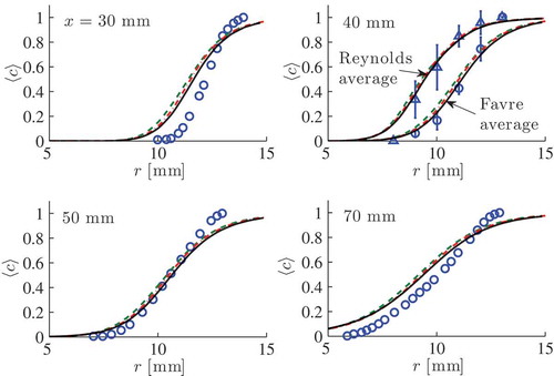
where is the Favre variance of , the resolved variance being obtained as . Furukawa et al. (2016) were also able to extract the Reynolds average from their experimental data, although it exhibited error bars larger than those for the Favre average. The experimental data for Reynolds averages were reported only for . The difference between the computed Reynolds and Favre averages for other locations are similar to that shown for and one can estimate this Reynolds average using the Favre average and its variance (to be discussed next) through Eq. (15). The significant difference between Favre- and Reynolds-averaged values observed in the figure implies that the variance of the progress variable in both the experiment and the LES is large. Since the flamelets are quasi-laminar, this variance is predominantly produced by combustion, which operates at the SGS level for the LES. All of the agreements between LES predictions and the experiment seen in Figure 11 are good in that the differences are less than the experimental uncertainties, which are similar to those shown for (Furukawa et al., 2016).

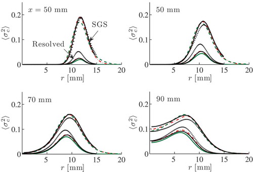
The radial variations of resolved and SGS variances are shown in Figure 12. The results appearing here from the 23M grid will be discussed in a later section. The SGS variance is nearly four to five times the resolved part for the location in the flame closest to the jet exit, and the resolved part is smaller than SGS part for all locations shown here. The relative contribution of the resolved part increases with increasing height because of the associated relative increase in the turbulence level and flame thickness. These observations suggest that models for deduced from a passive-scalar scenario would be inappropriate. This is expected in low turbulence as such models, typically written as (Pierce and Moin, 1998), require the most of the energy to be at super-grid scale. However, this model is shown to be inappropriate even for flames with high turbulence levels (Langella and Swaminathan, 2015) as it does not consider the effect of the flame, which is typically at subgrid level in LES. Hence, its use for LES of premixed combustion should be discouraged.

Figure 12. Resolved and SGS variance of the progress variable. Lilly model, Eq. (11) (dashed line), Pope model, Eq. (12) (continuous line), and Colin et al. model, Eq. (13) (dash-dotted line). The dotted line is for 23M grid with Pope model.

Furukawa et al. (2016) also extracted from their data an average turbulent-flame central contour based on a Favre-averaged progress variable of 0.5 and an average turbulent-flame thickness based on the radial extent of radial-velocity bimodality. Figure 13 compares those results with LES predictions, using and in the computations. Again, the dashed curves marked as 23M will be discussed in a later section. The agreements are seen to be good in that none of the differences between experimental and LES results exceed experimental uncertainties. Furukawa et al. (2016) refer to the bulge seen in the range of the experimental results at the top of Figure 13 as a “bubble,” indicating that there is some experimental evidence for the associated double inflection point in the contour. They indicate, however, that the experimental uncertainties are large enough that one cannot be sure that this “bubble” exists. The LES does not exhibit this “bubble.” The flame-brush thickness predicted by the LES is slightly thinner with the Lilly and Colin models, consistent with the results in Figure 11, but the differences are small, and predictions are in agreement with the experiment, within experimental error.

In summary, the results suggest that the flame statistics are not influenced by the choice of modeling if the parameter is chosen carefully to match the measured flame length and the SGS variance of is obtained using its transport equation. Thus, the unstrained flamelet model can be used with careful selection of SGS modeling to capture these physical aspects.

Bimodality of radial velocity PDFs

Figure 14 shows PDFs of velocities at five radial positions that span the turbulent flame brush, at a representative mid-flame height of 50 mm. The LES results shown are those for the resolved part only. A good agreement is seen between the LES results and measurements for the tangential velocity PDF. The computed axial velocity PDF also compares well the measurement except for the small shift in the location of the peak. This shift is consistent with the results in Figure 10. For the radial component, however, the experiment exhibits a strong bimodality in the center of the turbulent flame that is not reflected in the simulation results. The LES does show skewness of the radial-velocity PDFs in the flame region, with a high-velocity tail near the fresh mixture and probably a low-velocity tail near of burned gas sides of the flame brush. Since the mean dilatation produces higher radial velocities in the burned gas, the skewness may arise from the occasional penetration of reacted mixture into the position at low average completion of combustion, as is seen in the computed time-dependent behavior. The bimodality at the measurement positions where it is seen, however, cannot come from these resolved-scale components with the practical grids used here. It is a subgrid phenomenon on these grids (indeed small-scale phenomenon for ultra fine grids or DNS) for the corrugated-flamelet regime, that is not present in any of the three subgrid velocity models tested here.

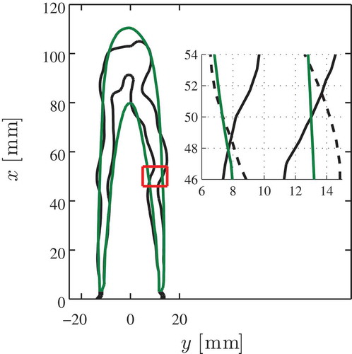
This radial-component bimodality, coming from flame intermittency, that is, back and forth flamelet movement in the radial direction, as suggested by Furukawa and Williams (2003), is strong at mm in the experiment. The computational results do not give this PDF because the filtered flame width is similar to the flame-brush width, as shown in Figure 15, and the flame-brush width is about 6 mm as shown in Figure 13b. This implies that the radial movement of the flame is significantly smaller than the filtered flame thickness and thus the probability of finding cells with intermediate values of is high. The bimodality can be seen only if sufficiently low and high values of are observed at a given point. Because of these reasons, it is not possible for the LES to capture the velocity fluctuations resulting from the flame intermittency.

Figure 13. The computed isolines of are compared to the experimental result in (a) along with the uncertainty for the measurements. A comparison of flame brush thickness is shown in (b). Lilly model, Eq. (11) (dashed line), Pope model, Eq. (12) (continuous line), and Colin et al. model, Eq. (13) (dash-dotted line). The dotted line is for 23M grid with Pope model.

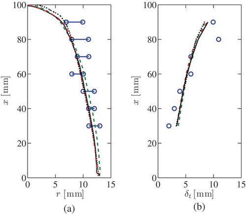
Figure 14. PDF of three velocity components at for various radial locations. Lilly model, Eq. (11) (dashed line), Pope model, Eq. (12) (continuous line), and Colin et al. model, Eq. (13) (dash-dotted line). The dotted line is for 23M grid with Pope model. Experimental data of Furukawa et al. (2016) are also shown for comparison.

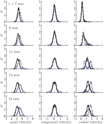
Figure 15. Isocontours of Favre-filtered (black lines) and Favre-averaged (green lines) progress variable at values 0.1 and 0.9 for the 5.3M grid. An enlarged view is shown for radial positions marked in Figure 14 in the inset. The Favre-filtered isoline is shown for two different times.

Further insight can be gleaned by considering the measured bimodal PDF as two Gaussians. The experimental data suggests that the means are and , and the variances are and , respectively, for the unburned and burned mixtures. The subscripts and denote the left (unburned mixture) and right (burned) parts of the PDF. The width of these two Gaussians, represented by the respective variances, are influenced by turbulence, and the separation of the two peaks are controlled by flame intermittency. The turbulence contribution is captured quite well in the simulations and this can be seen by writing the joint PDF of and as , where is the sample space variable for . If one presumes the marginal PDF to be BML as has been done by Libby and Bray (1980) and Bray et al. (1985) then:

16

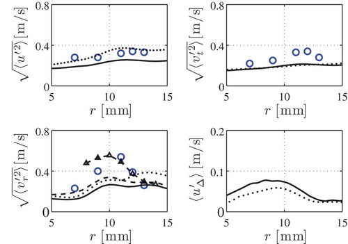
where is the burning mode part of the marginal PDF, , which can be evaluated by integrating the beta PDF used for reaction-rate closure between the limits of and 0.95, but it is not easy to get as it is related to the effects of combustion on SGS velocity fluctuation. The sum compares well with the computed rms value of 0.26 at shown in Figure 16 (solid line). Nearly 78% of the total variance, , at this radial location comes from the flame intermittency (evaluated using the distance between the peak locations in the experimental PDF), which suggests that the subgrid part must be . Even with the gross assumption that the total contributes to , the computed variance is increased by only a small amount of , which is negligible compared to . One can artificially include the intermittency effect by increasing the size of data sampling region to 6 mm as shown in Figure 16 (symboled line). Since this is artificial the corresponding PDF is not shown in Figure 14.

Figure 16. RMS and SGS velocity profiles for 5.4M (continuous line) and 23M (dotted line) grids are compared to the experimental data (symbols) for x = 50 mm. The dashed line for rms of radial velocity includes . The role of flame intermittency is shown by the symboled line by increasing the sampling region intentionally.

The maximum error for is found to be less than 2% although the difference between measured and computed values in Figure 16 for the axial velocity rms seems high. There is some difference for the tangential component, which results from the flame intermittency. This contribution will be highly anisotropic in the corrugated-flamelet regime and thus including fully for the radial component is not justifiable. Similarly, other corrections such as Deardorff correction (Deardorff, 1971; Ribault et al., 1999) for the rms values cannot be used because they generally require isotropy, which is not met in flames. Therefore, improved SGS velocity modeling strategies are required to capture the strong anisotropic effects of flame intermittency in practical LES.

Influence of numerical grid

Strictly, one should include the contribution of SGS fluctuations when constructing the velocity PDF, and these fluctuations are unavailable in LES framework unless the grid is refined to a level so that they becomes negligible. Indeed, one can refine the grid to have , so the filtered flame width becomes comparable to the flamelet thickness to capture the bimodal behavior. The minimum filter width based on the numerical cell volume is about for the 5.2M grid and to have a filter width of , which is comparable to the experimental resolution length, one needs a grid with about 120M cells, which would be a very expensive calculation and thus it is not attempted here. However, another grid with about 23M cells is used to test the sensitivity of the statistics discussed above.

The first-order statistics obtained using the 23M grid are very similar to those obtained from the 5.4M grid (for example, see contour shown in Figure 13), and thus they are not shown here. The second-order statistics show some sensitivity to grid resolution as seen in Figure 16. Since the filter size decreases with an increase in grid resolution, the SGS velocity fluctuations are expected to decrease, which is seen in this figure. However, values are still high compared to the resolved rms values for the three velocity components, and this is because the flame effects are responsible for the predominant part of the SGS kinetic energy in these regions. The resolved rms of axial velocity fluctuation for the 23M grid compares reasonably well with the experimental data, the tangential component does not show any sensitivity, and there is some improvement for the radial component. There is, however, a substantial difference between the computed and measured because of the missing subgrid part, which is related to the flame intermittency effects, as noted above. The improvements in the rms value for the radial component is reflected in the PDFs shown in Figure 14 for locations inside the flame brush.

The SGS variance, , does not seem to be sensitive to the grid resolution and the resolved part increases with grid resolution as one would expect. The difference in the resolved part also becomes less sensitive to the grid further downstream. All of these points can be observed in results for the 23M grid shown in Figure 12. This suggests that the SGS combustion process is captured well by the reaction-rate closure used for this study. However, the influence of the flame intermittency and resulting acceleration effects on the SGS velocity fluctuation is not represented directly by the commonly used SGS velocity models. Thus, the experimentally observed bimodality of the radial velocity is not captured fully.

Summary and conclusions

A non-piloted Bunsen flame of a propane-air mixture with an equivalence ratio of 0.85 and low turbulence level, lying in the corrugated-flamelet regime, has been simulated using an unstrained-flamelet model for the filtered reaction rate. The turbulence-chemistry interaction is driven by flame-induced effects, which is different from the shear-produced turbulence effects in standard piloted jet flames. Thus, the modeling of SGS velocity is expected to play a role, and three different models treating the dilation effects differently are considered. The SGS variance of a reaction-progress variable required for the presumed PDF is obtained by using its transport equation. The dissipation rate required for this equation is closed by applying an algebraic model developed by Dunstan et al. (2013). The grid sensitivity of the statistics is also assessed using 5.4M and 23M grids.

The computed statistics compare reasonably well with the experimental results, and the grid sensitivity of the statistics is found to be negligible. This suggests that the unstrained flamelet closure is robust and adequate for practical LES of premixed combustion. There is an underprediction of the variance of the radial component of velocity in the central part of the flame, where the respective PDF was observed to be bimodal in experiments. Detailed analyses of LES and experimental PDFs suggest that the turbulence effects are captured quite well in the LES, whereas the effects of flamelet intermittency is not. These strong and anisotropic effects in the corrugated-flamelet regime of combustion are not represented by the commonly used SGS velocity models, and improved models are required.

Acknowledgments

The authors express their gratitude to EPSRC, Siemens, and Rolls-Royce for their support.

Funding

This work is funded by grant EP/I027556/1 from EPSRC. The contribution of the third author followed from support by the US AFOSR through grant FA9550-12-1-0138.

Additional information

Funding

This work is funded by grant EP/I027556/1 from EPSRC. The contribution of the third author followed from support by the US AFOSR through grant FA9550-12-1-0138.

References

- Anand, M., Zhu, J., Connor, C., and Razdan, M. 1999. Combustor flow analysis using an advanced finite-volume design system. In International Gas Turbine and Aeroengine Congress and Exhibition, ASME, Indianapolis, IN, Vol. 99-GT, p. 273.
- Bardina, J., Ferziger, J.H., and Reynolds, W.C. 1980. Improved subgrid scale models for large-eddy simulation. Am. Inst. Aeronaut. Astronaut., 80, 1357.
- Bray, K.N.C., Libby, P.A., and Moss, J.B. 1985. Unified modeling approach for premixed turbulent combustion—Part I: General formulation. Combust. Flame, 61, 87–102.
- Butz, D., Gao, Y., Kempf, A.M., and Chakraborty, N. 2015. Large eddy simulations of a turbulent premixed swirl flame using an algebraic scalar dissipation rate closure. Combust. Flame, 162, 3180–3196.
- Cant, R.S. 2011. RANS and LES modelling of turbulent combustion. In T. Echekki and E. Mastorakos (Eds.), Turbulent Combustion Modelling: Advances, New Trends and Perspectives, Springer, Heidelberg, pp. 63–87.
- Chakraborty, N., and Swaminathan, N. 2007. Influence of the Damköhler number on turbulence-scalar interaction in premixed flames. II. Model development. Phys. Fluids, 19, 045104-1-11.
- Charlette, F., Meneveau, C., and Veynante, D. 2002. A power-law flame wrinkling model for LES of premixed turbulent combustion, Part ii: Dynamic formulation. Combust. Flame, 131, 181–197.
- Colin, O., Ducros, F., Veynante, D., and Poinsot, T.J. 2000. A thickened flame model for large eddy simulations of turbulent premixed combustion. Phys. Fluids, 12, 1843.
- Colucci, P.J., Jaberi, F.A., Givi, P., and Pope, S.B. 1998. Filtered density function for large eddy simulation of turbulent reacting flows. Phys. Fluids, 10, 499.
- Cook, A.W. 1997. Determination of the constant coefficient in scale similarity models of turbulence. Phys. Fluids, 9, 1485.
- De, A., and Acharya, S. 2009. Large eddy simulation of a premixed Bunsen flame using a modified thickened-flame model at two Reynolds number. Combust. Sci. Technol., 181(10), 1231–1272.
- Deardorff, J.W. 1971. On the magnitude of the subgrid scale eddy-viscosity coefficient. J. Comput. Phys., 7, 120–133.
- Domingo, P., Vervisch, L., Payet, S., and Hauguel, R. 2005. DNS of a premixed turbulent V flame and LES of a ducted flame using FSD-PDF subgrid scale closure with FPI-tabulated chemistry. Combust. Flame, 143, 566–586.
- Doormaal, J.P. van and Raithby, G.D. 1984. Enhancements of the simple method for predicting incompressible fluid flows. Numer. Heat Transfer, 7(2), 147–163.
- Dunstan, T.D., Minamoto, Y., Chakraborty, N., and Swaminathan, N. 2013. Scalar dissipation rate modelling for large eddy simulation of turbulent premixed flames. Proc. Combust. Inst., 34, 1193–1201.
- Duwig, C. 2007. Study of a filtered flamelet formulation for large eddy simulation of premixed turbulent flames. Flow Turbul. Combust., 79(4), 433–454.
- Fiorina, B., Veynante, D., and Candel, S. 2015. Modeling combustion chemistry in large eddy simulation of turbulent flames. Flow Turbul. Combust., 94, 3–42.
- Furukawa, J., Noguchi, Y., Hirano, T., and Williams, F.A. 2002. Anisotropic enhancement of turbulence in large-scale, low-intensity turbulent premixed flames. J. Fluid Mech., 462, 209–243.
- Furukawa, J., and Williams, F.A. 2003. Flamelet effects on local flow in turbulent premixed Bunsen flames. Combust. Sci. Techol., 175, 1835–1858.
- Furukawa, J., Yoshida, Y., Amin, V., and Williams, F.A. 2013a. Changes of gas velocities in passing through flamelets in a premixed turbulent Bunsen flame. Combust. Sci. Technol., 185, 200–211.
- Furukawa, J., Yoshida, Y., and Williams, F.A. 2013b. Evolution of gas velocities behind flamelets in a premixed turbulent Bunsen flame. Combust. Sci. Technol., 185, 661–671.
- Furukawa, J., Yoshida, Y., and Williams, F.A. 2016. Structures of methane-air and propane-air turbulent premixed Bunsen flames. Combust. Sci. Technol., 188(9), 1538–1564.
- Gao, Y., Chakraborty, N., and Swaminathan, N. 2014a. Algebraic closure of scalar dissipation rate for large eddy simulations of turbulent premixed combustion. Combust. Sci. Technol. 5 186(10), 1309–1337.
- Gao, Y., Chakraborty, N., and Swaminathan, N. 2014b. Scalar dissipation rate transport in the context of LES for turbulent premixed flames with non-unity Lewis number. Flow Turbul. Combust., 93, 461–486.
- Gao, Y., Chakraborty, N., and Swaminathan, N. 2015. Dynamic closure of scalar dissipation rate for large eddy simulations of turbulent premixed combustion: A direct numerical simulations analysis. Flow Turbul. Combust., 95, 775–802.
- Germano, M., Piomelli, U., Moin, P., and Cabot, W.H. 1991. A dynamic subgrid-scale eddy viscosity model. Phys. Fluids A, 3, 1760.
- Gicquel, L.Y.M., Staffelbach, G., and Poinsot, T. 2012. Large eddy simulations of gaseous flames in gas turbine combustion chambers. Prog. Energy Combust. Sci., 38, 782–817.
- Gubba, S.R., Ibrahim, S.S., and Malalasekera, W. 2012. Dynamic flame surface density modelling of flame deflagration in vented explosion. Combust. Explos. Shock Waves, 48, 393–405.
- Kee, R.J., Grcar, J.F., Smooke, M.D., and Miller, J.A. 1985. A fortran program for modeling steady laminar one-dimensional premixed flames. Technical Report. SAND85-8240. Sandia National Labortories.
- Kemenov, K.A., Wang, H., and Pope, S.B. 2012. Turbulence resolution scale dependence in large-eddy simulations of a jet flame. Flow Turbul. Combust., 88, 529–561.
- Klein, M., Sadiki, M., and Janicka, J. 2002. A digital filter based generation of inflow data for spatially developing direct numerical or large eddy simulations. J. Comput. Phys., 186, 652–665.
- Kolla, H., Rogerson, J.W., Chakraborty, N., and Swaminathan, N. 2009. Scalar dissipation rate modeling and its validation. Combust. Sci. Technol., 181, 518–535.
- Kolla, H., and Swaminathan, N. 2010. Strained flamelets for turbulent premixed flames, II: Laboratory flame results. Combust. Flame, 157, 1274–1289.
- Landenfeld, T., Sadiki, A., and Janicka, J. 2002. A turbulence-chemistry interaction model based on a multivariate presumed beta-PDF method for turbulent flames. Flow Turbul. Combust., 68, 111–135.
- Langella, I., and Swaminathan, N. 2015. Unstrained and strained flamelets for LES of premixed combustion. Combust. Theor. Model., 20(3), 410–440.
- Langella, I., Swaminathan, N., Gao, Y., and Chakraborty, N. 2015. Assessment of dynamic closure for premixed combustion LES. Combust. Theor. Model., 19(5), 628–656.
- Lecocq, G., Richard, S., Colin, O., and Vervisch, L. 2010. Gradient and counter-gradient modeling in premixed flames: Theoretical study and application to the LES of a lean premixed turbulent swirl-burner. Combust. Sci. Technol., 182, 465–479.
- Lecocq, G., Richard, S., Colin, O., and Vervisch, L. 2011. Hybrid presumed pdf and flame surface density approaches for large-eddy simulation of premixed turbulent combustion: Part 1: Formalism and simulation of a quasi-steady burner. Combust. Flame, 158, 1201–1214.
- Libby, P.A., and Bray, K.N.C. 1980. Implications of the laminar flamelet model in premixed turbulent combustion. Combust. Flame, 39, 33–41.
- Lilly, D.K. 1967. The representation of small-scale turbulence in numerical simulation experiments. In H. H. Goldstine (Ed.), Proceedings of the IBM Scientific Computing Symposium on Environmental Sciences, IBM, Yorktown Heights, NY, pp. 195–210.
- Lilly, D.K. 1992. A proposed modification of the Germano subgrid scale closure method. Phys. Fluids A, 4, 633–635.
- Ma, T., Gao, Y., Kempf, A.M., and Chakraborty, N. 2014. Validation and implementation of algebraic LES modelling of scalar dissipation rate for reaction rate closure in turbulent premixed combustion. Combust. Flame, 161, 3134–3153.
- Métais, O., and Lesieur, M. 1992. Spectral large-eddy simulation of isotropic and stably stratified turbulence. J. Fluid Mech., 239, 157–194.
- Moureau, V., Domingo, P., and Vervisch, L. 2011. From large-eddy simulation to direct numerical simulation of a lean premixed swirl flame: Filtered laminar flame-PDF. Combust. Flame, 158, 1340–1357.
- Nambulli, S., Domingo, P., Moureau, V., and Vervisch, L. 2014. A filtered-laminar-flame PDF sub-grid-scale closure for LES of premixed turbulent flames: II. Application to a stratified bluff-body burner. Combust. Flame, 161, 1775–1791.
- Nguyen, P., Vervisch, L., Subramanian, V., and Domingo, P. 2010. Multidimensional flamelet-generated manifolds for partially premixed combustion. Combust. Flame, 157, 43–61.
- Nicoud, F., Toda, H.B., Cabrit, O., Bose, S., and Lee, J. 2011. Using singular values to build a subgrid-scale model for large eddy simulation. Phys. Fluids, 23, 085106.
- Peters, N. 2000. Turbulent Combustion, Cambridge University Press, Cambridge, UK.
- Pierce, C.D., and Moin, P. 1998. A dynamic model for subgrid-scale variance and dissipation rate of a conserved scalar. Phys. Fluids, 10(12), 3041–3044.
- Pitsch, H. 2006. Large-eddy simulation of turbulent combustion. Annu. Rev. Fluid Mech., 38, 453–482.
- Poinsot, T.J., and Veynante, D. 2005. Theoretical and Numerical Combustion, Edwards.
- Pope, S.B. 2000. Turbulent Flows, Cambridge University Press, Cambridge, UK.
- Ribault, C.L., Sarkar, S., and Stanley, S. 1999. Large eddy simulation of a plane jet. Phys. Fluids, 11, 3069.
- Rieth, M., Proch, F., Stein, O.T., Pettit, M.W.A., and Kempf, A.M. 2014. Comparison of the Sigma and Smagorinsky LES models for grid generated turbulence and a channel flow. Compute. Fluids, 99, 172–181.
- Ruan, S., Swaminathan, N., and Darbyshire, O. 2014. Modelling of turbulent lifted jet flames using flamelets: A priori assessment and a posteriori validation. Combust. Theor. Model. 18(2), 295–329.
- Sung, C.J., Li, B., Wang, H., and Law, C.K., 1998. Structure of sooting limits in counterflow methane/air and propane/air diffusion flames from 1 to 5 atmospheres. Proc. Combust. Inst., 27(1), 1523–1529.
- Swaminathan, N., and Bray, K.N.C. 2011. Fundamentals and challenges. In N. Swaminathan and K. N. C Bray (Eds.), Turbulent Premixed Flames, Cambridge University Press, Cambridge, UK, pp. 1–40.
- UC San Diego. 2014. Chemical-kinetic mechanisms for combustion applications, mechanical and aerospace engineering (combustion research). Available at: http://combustion.ucsd.edu.
- Vreman, A.W. 2004. An eddy-viscosity subgrid-scale model for turbulent shear flow: Algebraic theory and applications. Phys. Fluids, 16, 3670.
- Vreman, A.W., Van Oijen, J.A., De Goey, L.P.H. and Bastiaans, R.J.M. 2009. Subgrid scale modelling in large-eddy simulation of turbulent combustion using premixed flamelet chemistry. Flow Turbul. Combust., 82, 511–535.
- Wang, G., Boileau, M., and Veynante, D. 2011. Implementation of a dynamic thickened flame model for large eddy simulations of turbulent premixed combustion. Combust. Flame, 158, 2199–2213.
- Wang, G., Boileau, M., Veynante, D., and Truffin, K. 2012. Large eddy simulation of a growing turbulent premixed flame kernel using a dynamic flame surface density model. Combust. Flame, 159(8), 2742–2754.
- Zhu, J. 1991. Low diffusive and oscillation-free convection scheme. Commun. Appl. Numer. Methods, 7, 225–232.
- Zhu, J., and Rodi, W. 1991. A low dispersion and bounded discretization scheme for finite volume computations of incompressible flows. Comput. Methods. Appl. Mech. Eng., 92, 87–96.