Structures of Methane-Air and Propane-Air Turbulent Premixed Bunsen Flames

ABSTRACT

Structures of turbulent Bunsen flames in the corrugated-flamelet regime were investigated by use of a three-color six-beam laser-Doppler velocimetry system. Four different mixtures with identical laminar burning velocities (0.34 m/s) were selected to facilitate comparisons—lean and rich methane, and lean and rich propane. A bimodal distribution, not previously reported in the literature on turbulent Bunsen flames, was observed in the radial component of gas velocity off-axis in the turbulent flame brush. Our previous measurements enabled the low-velocity mode to be identified as velocity fluctuations of the unburned mixture and the high-velocity mode as fluctuations of the burned-gas radial velocity. Favre-averaged and Reynolds-averaged reaction-progress variables were then calculated from these bimodal distributions, identifying an initially unexpected region near the flame tips where, at a fixed radius, the average progress variable decreased (rather than increasing) with increasing height over a short distance, likely through enhanced flamelet flapping, which has not been predicted by modeling but which appears to occur quite generally for sufficiently tall turbulent Bunsen flames in quiescent ambient environments, for the corrugated-flamelet regime. Conditioned and unconditioned Favre-average velocity components and intensities also were calculated from the data for future tests of modeling. The distributions of the progress variables also clearly showed that the turbulent burning velocity of the rich propane flame was appreciably larger than that of any of the other three, as was its radial flame-brush thickness at any given height, and its high-radial-velocity mode had a higher average velocity magnitude than the others. Similarly, the turbulent burning velocity and flame-brush thickness appear to be smaller for the lean propane flame. These differences can be attributed to influences of preferential oxygen diffusion to turbulence-induced flamelet bulges, not included in existing modeling approaches, for the rich propane flames, and to a corresponding inhibition of fuel diffusion to the bulges in the lean flames. The former phenomenon is related to but different from the well-known cellular-flamelet instability, these effects occurring for flames that are stable to diffusive-thermal disturbances. It was concluded that a greater fraction of the total amount of heat release occurs in the upstream half of the turbulent flame brush in the rich propane flame, producing enhanced flow divergence in the upstream region, while the reduced ability of the slowly diffusing fuel to reach bulges in the lean flame generates the opposite effect. The results point to directions in which turbulent-combustion modeling needs to be improved, and an approach to modeling this type of preferential-diffusion effect is suggested.

KEYWORDS:

• Flame structure
• Laser-Doppler velocimetry
• Preferential diffusion
• Turbulent premixed flame

Introduction

Structures of turbulent flames differ considerably in different regimes of turbulent combustion (Peters, 2000). Ordinary premixed turbulent Bunsen flames of gaseous hydrocarbon fuels in the laboratory often are in the corrugated-flamelet regime (Peters, 2000), as was the case in our earlier work (Furukawa et al., 2002). Although such flames have been investigated experimentally by Schlieren, shadowgraph, and visible-emission techniques for more than 60 years (Bollinger and Williams, 1949; Hottel et al., 1953; Karlovitz et al., 1953), unexpected aspects of their structures continue to be discovered by experimental methods ranging from the use of electrostatic probes (Furukawa et al., 2002, 2010, 2013a, 2013b) to laser-sheet Mie-scattering tomography (Kobayashi et al., 1996, 1997, 1998), to combined Rayleigh scattering and planar OH laser-induced fluorescence (LIF; Chen and Bilger, 2001, 2002; Frank et al., 1999), to laser-Doppler velocimetry (LDV; Furukawa et al., 2002, 2013a, 2013b) and particle-image velocimetry (PIV; Frank et al., 1999; Pfadler et al., 2009; Steinberg et al., 2009). Many of these techniques have been applied to turbulent flames in the thin-reaction-zone regime or in the broken-flamelet regime, but flamelet structures in those regimes depart substantially from the structures of planar-laminar flamelets, and their stabilization as Bunsen flames generally requires the use of pilot burners (e.g., Frank et al., 1999). The present study is restricted to the corrugated-flamelet regime, with the objective of identifying new aspects of turbulent Bunsen-flame structures in that regime, as well as providing additional information to test existing concepts. More precisely, conditions are near the borderline of the wrinkled-flamelet (also called weak-turbulence) regime, far from the thin-reaction-zone regime, so that Markstein numbers should be appropriate for describing effects of the turbulence on the flamelets.

Based on this viewpoint, we extend our earlier work, in which we have made measurement of flow fields (Furukawa et al., 2002), flamelet motion (Furukawa et al., 2010), and flame-flow interactions (Furukawa et al., 2013a, 2013b). Scatter plots for flamelet velocity vectors were obtained for flamelets passing an electrostatic probe in the direction of fresh-to-burned and, separately, burned-to-fresh directions, correlations between magnitudes and directions of flamelet velocities were measured, and probability distributions were generated for magnitudes and directions of flamelet velocity vectors, as well as identifying flamelet influences on Kolmogorov spectra (Furukawa et al., 2002). Our previous study of flamelet motions (Furukawa et al., 2010) revealed significant differences between rich propane Bunsen flames and the corresponding lean propane flames (or lean or rich methane flames), all with nearly the same laminar burning velocities. It was hypothesized in that work that the differences arise from turbulence-produced flamelet wrinkling, followed by preferential oxygen diffusion to protruding wrinkles, thereby enhancing the average flamelet propagation velocity. Since gas velocities were not measured in that work, corroborating gas-velocity evidence was not available. In the present study LDV data are acquired to further test the hypothesis.

The objective of the present study is to provide velocity-field information that can be of help in future modeling efforts in flamelet regimes. Over the years there has been extensive modeling work devoted to these regimes, beginning with studies of Spalding, and later Bray and co-workers. This material has been reviewed, for example, in books edited by Libby and Williams (1980, 1994) and written by Peters (2000). Many different modeling approaches have been explored, starting with RANS, now including flamelets, and more recently emphasizing LES. In view of experimental challenges, DNS methods have increasingly been used for such investigation (Chakraborty et al., 2011a, 2011b; Haworth and Poinsot, 1992; Kolla et al., 2009, 2010; Nikolaou et al., 2014; Poinsot and Veynante, 2001; Zhang and Rutland, 1995). Because thin flamelets stress full DNS capabilities, such studies currently more often address the thin-reaction-zone regime (Chakraborty et al., 2011b). There is extensive modeling of that regime in the recent literature, with less attention being given nowadays to flamelet regimes. Outstanding questions nevertheless remain for all regimes, and comparisons of predictions with experiment, as well as with DNS results, can be helpful in testing modeling assumptions.

Beyond weak-turbulence or wrinkled-flamelet regimes, flamelet structures are modified least by turbulence in the corrugated-flamelet regime, so that classical concepts for modeling turbulent combustion can be tested most thoroughly in that regime. A number of the modeling approaches rely on the introduction of a reaction-progress variable C, related to the fraction of time that the burned gas is present at any given position in the flow. In the extreme limit of flamelets of zero thickness, either the fresh mixture or burned products are present at every point. Associated modeling is based on the assumption that flamelets are present at any point only for a small fraction of the time as, for example, in the pioneering Bray–Moss–Libby model, which uncovered the existence of counter-gradient diffusion and is of continuing significance today (Peters, 2000; Libby and Williams, 1994). There are a number of potentially important research directions that, for instance, can apply to this regime (Bilger, 2000), and data on C can test predictions derived from these different directions of research. Our LDV measurements revealed unexpectedly that our data can provide local average values of C, under the assumption that the measurements are essentially only in fresh or burned gas. Individual LDV data (Furukawa et al., 2002, 2013a, 2013b) verify that, in fact, more than 85% of the data points reside in either fresh or burned gas, so that the error in this assumption is not large. Therefore, results for averages of C are extracted from the measurements to aid in future tests of predictions. In addition, directions for improvements in modeling are suggested on the basis of these results.

Experimental apparatus, instrumentation, and procedures

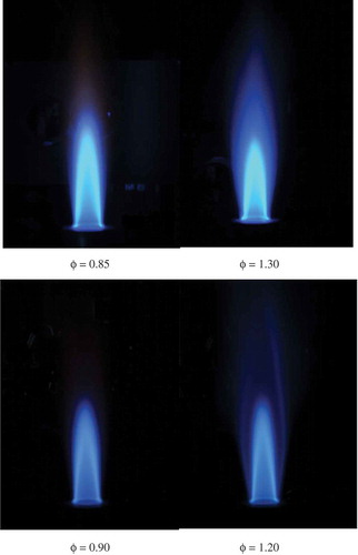
The burner used in the present study is the same cylindrical burner (26 mm in diameter) that was employed in our previous investigations (Furukawa et al., 1994, 1998, 2002, 2010, 2013a, 2013b). Propane and methane are selected as the fuel used in the present study. The fuel, oxygen, and inert all have approximately the same diffusivity, except for propane, whose diffusivity is smaller than that of oxygen enabling preferential diffusion to occur in the propane flames. Values of the equivalence ratio ϕ employed for propane-air flames were 0.85 and 1.30 and for the methane-air flames values of ϕ were 0.90 and 1.20. These values correspond to identical laminar burning velocities S_L of about 0.34 m/s, according to results of Vagelopoulos and Egolfopoulos (1998). Although different methods produce somewhat different burning velocities, those differences are likely to be small enough to be negligible for the purposes of the present studies. A uniform propane-air or methane-air mixture was supplied to the burner at an average cold-flow exit velocity of 4.0 m/s, corresponding to fully developed turbulent pipe flow at a Reynolds number of about 7000. The characteristics of the turbulence were examined by a hot-wire anemometer in cold flow at the centerline position. In the hot-flow experiments, sufficient time for establishing steady, statistically stationary conditions was allotted prior to beginning measurement. The average cold-flow velocity U on the centerline was 4.5 m/s, the turbulence intensity (root-mean-square velocity fluctuations) u’ was 0.22 m/s, the integral scale L_x was 10.9 mm, the Taylor scale λ_x was 3.5 mm, the Kolmogorov scale η was 260 μm, and the Reynolds number R_L based on the integral scale was 154 (Furukawa et al., 2002). With the flame present, reactant heating by heat transfer from the tube wall increases U (N. Swaminathan, private communication, 2014); infrared measurements indicated that the maximum wall temperature would be as much as 100 K above ambient, with a vertical gradient on the order of 1 K/mm to 2 K/mm. The laminar-flame thickness and Karlovitz number, as defined by Peters (2000, p. 78) are 53 μm and 0.04, placing the system well into the flamelet regime.

Figure 1 shows visible-image photographs of the four flames investigated. All four are blue, without yellow, while the propane flame is, of course, a bit brighter, as well as greener in the rich case, as expected. Except for the rich propane flame, which is seen to be shorter, all appear to have approximately the same height, although the lean propane flame may be a little taller. The weak diffusion flames surrounding the two rich flames can be seen in the photographs and appear to be far enough away from the premixed flames that their influences on the interior premixed-flame structures should be negligible.

Figure 1. Direct photographs of propane-air (upper) and methane-air (lower) flames.

An LDV system (Artium LDV-300SC), composed of three semiconductor lasers operating at wavelengths 491 nm (100 mW), 532 nm (150 mW), and 561 nm (100 mW), along with a three-color, six-beam, forward-scattering optical system, and three Doppler signal analyzers provided the 3D measurement of the local gas velocity. The measuring volume of this 3D LDV system is a sphere of approximately 0.2 mm in diameter, determined by the intersection of two football-like measuring volumes of the 2D and 1D transmitters, whose length and diameter are 2.2 mm and 0.2 mm, respectively, which is smaller than typical LES grid sizes. The micron-size scattering particles, seeded in the unburned mixture stream, were obtained from SiO₂ powder. Radial-traverse measurements were conducted at different fixed heights, from h = 30 mm to as much as 90 mm above the burner exit, at every 1 mm in the radial direction. Vertical-traverse measurements along the centerline also were obtained.

Probability distributions of velocity components

Representative probability distributions of the axial, tangential, and radial components of the gas velocity obtained in the present study are shown in Figure 2. The results of this radial traverse, at 50 mm above the burner exit of the lean propane-air flame, are qualitatively similar to the results of the traverses at the mid-turbulent-flame heights for all four flames. In the figures, N and N_s represent the number of samples in a bin of interval 0.04 m/s and the total number of samples, respectively. Mono-modal distributions are observed in the axial and tangential components of the gas velocity. The axial component is distributed approximately symmetrically between 4.0 m/s and 6.5 m/s, with its peaks at 5.5 m/s in this case; such nearly symmetrical distributions of the axial component are characteristic of the results obtained at all heights in all of the flames. The tangential component is distributed symmetrically about 0 m/s, as it should be, according to the symmetry of the experiment; the slight departures from exact symmetry that are detectable here are typical of all of the data and reflect inaccuracies in alignment and insufficiencies in data rates, seen here to be very small. The range of fluctuations of the axial and tangential components increase with increasing radius at these mid-turbulent flame brush locations in all of the flames, until the radial position begins to emerge from the flame brush, at which point the range begins to decrease as is reflected especially in root-mean-square plots of velocity fluctuations for the tangential components of other data (not shown).

Figure 2. Change in the probability distributions of the axial (left), tangential (center), and radial (right) components of the gas velocity at 50 mm height in propane-air flames with ϕ = 0.85.

Contrary to the axial and tangential components, the radial component of the gas velocity is characterized by a bi-modal distribution in the interior of the flame brush. In this example, when the radial position r is less than 7 mm, a mono-modal distribution, which is composed almost completely of the velocity fluctuations of the unburned mixture, is observed in the radial component. When the radial position r is between 7 mm and 12 mm, a bimodal distribution, composed of a low-velocity mode and a high-velocity mode, is observed in the radial component. As the radial position r increases, the number of samples in the low-velocity mode decreases, and the number of samples in the high velocity mode increases. The zone in which the bimodal distribution is observed can be interpreted as the turbulent flame brush, with the low-velocity data coming primarily from measurements made when the fresh mixture is present and the high-velocity data corresponding mainly to the presence of the burned gas. When the radial position r is larger than 12 mm in this case, a mono-modal distribution again develops in this radial component, which now is dominated by the velocity fluctuations of the burned gas. This type of development of bi-modality in LDV data does not appear to have been observed previously.

Figure 3 illustrates this effect by showing a flamelet of roughly sinusoidal shape traveling vertically upward rapidly while moving horizontally back and forth more slowly, as reasoned in an earlier work (Furukawa and Williams, 2003). Flamelets of this kind pass the stationary measuring volume of the LDV alternately in the burned-to-unburned then unburned-to-burned directions (Furukawa et al., 2013a). When the radial position r is less than 7 mm, the measuring volume of the LDV is always in the fresh mixture, so that only unburned gas velocities are detected. When the radial position r is between 7 mm and 12 mm, the measuring volume of the LDV resides within the turbulent flame brush. When the measuring volume is near the inner side (unburned-mixture side) of the turbulent flame brush, as shown in Figure 3a, it remains longer in the fresh mixture, so that a larger number of samples of the unburned mixture velocity is recorded. On the other hand, when the measuring volume is near the outer side (burned-gas side) of the turbulent flame brush, as shown in Figure 3b, it stays longer in the burned-gas stream, so that consequently a larger number of samples of the burned-gas velocity is recorded. Therefore, as the radial position r increases, the number of samples of the unburned-mixture velocity decreases, while the number of samples of the burned-gas velocity increases. When the radial position r is larger than 12 mm, the measuring volume of the LDV is always in the burned gas, and only the burned-gas velocity is detected.

Figure 3. Illustration of a flamelet passing the measuring position.

It may be difficult to understand why a bi-modal distribution appears only of the radial velocity component. Since the tangential component of velocity is distributed symmetrically about 0 m/s, the bi-modal distribution, composed of the low-velocity mode of the fresh mixture and the high-velocity mode of the burned gas, can appear only in the vertical or radial velocity-component distributions. Figure 4 is a diagram of the gas-velocity change across flamelets for those two components. The gas velocity increases in a direction perpendicular to the flamelet because of thermal expansion, as we have previously explained (Furukawa and Williams, 2003), leading to anisotropic enhancement of gas flow across the flamelet (Furukawa et al., 2002). The direction in which the gas velocity increases most depends on the flamelet orientation. When the polar angle θ of the flamelet velocity vector in the spherical coordinate system is less than 45°, the gas velocity increases more in the vertical direction, as shown in Figure 4a. On the other hand, when the polar angle θ of the flamelet velocity vector is larger than 45°, the gas velocity increases more in the horizontal direction, as shown in Figure 4b. We found in a previous study (Furukawa et al., 2010) that, under conditions typical of our experiment, the polar angle θ of the flamelet velocity vector exceeds 45°, indicating that the gas velocity increases more in the horizontal direction and less in the vertical direction. The bimodality in the radial component (rather than the vertical component) thus arises from the fact that the gas flow is bent outward more than upward across the flamelet; that is, the surfaces of the flamelets are more nearly vertical sheets than horizontal sheets, as may also be inferred from the Schlieren images of Kobayashi et al. (1997) for similar conditions. This is also the source of the overall flow divergence in the turbulent flame brush.

Figure 4. Illustration of gas-velocity change across the flamelets. V_gu and V_gb denote the velocity vectors in the fresh and burned mixtures, respectively, and θ is the polar angle of the velocity vector of the flamelet, less than 45° on the left and greater than 45° on the right.

It is interesting to compare the shapes of the distributions of the radial velocity components for the flames of the four different mixtures in the center of the flame brush where the bimodal peaks are of approximately equal areas. This position occurs where the root-mean-square tangential velocity component is at maximum and is found at slightly different locations in each flame. Figure 5 shows such a comparison. It can be seen from this figure that the distributions are quite similar for both the lean and rich methane flames but differ appreciably for the lean and rich propane flames. The distributions for the lean propane flame, in fact, resemble those of the methane flames more than they resemble that of the rich propane flame. The low-velocity mode for the rich propane flame is similar to the other peaks, but its high-velocity mode is much broader and extends to higher velocities. This is consistent with the turbulence preferentially enhancing individual flamelet propagation in rich propane flames, as mentioned in the introduction and suggested earlier (Furukawa et al., 2010). This effect enhances the upstream flow divergence in that flame and will be discussed much more thoroughly in the following sections.

Figure 5. Probability distributions of the radial component of gas velocity at the radial position where the root mean square tangential component of velocity is maximum for methane flames of ϕ = 0.9 and 1.20 and propane flames of ϕ = 0.85 and 1.3 from top to bottom at 50 mm above the burner exist.

The progress variable

As indicated at the end of the introduction, the bi-modal LDV data for the radial component of velocity can be employed to obtain estimates of local average values of the progress variable C. A number of assumptions are required in making such estimates. First and foremost is the assumption that the seed particles follow the gas motion with negligible slip velocities. This has been shown to be an accurate assumption, even as the seed particles pass through flamelets (Furukawa et al., 2002, 2013a). Given this behavior, the seed-particle number density remains proportional to the gas density (Furukawa et al., 2002), so that the data rates in the fresh and burned mixtures are proportional to their respective gas densities. This means that, if averages are calculated directly from distributions such as those in Figures 2 and 5, then they are Favre averages. As the radial position r of the measuring volume of the LDV increases, the number of samples of the velocity fluctuations recorded in the unburned mixture decreases, while the number of samples of velocity fluctuation recorded in the burned gas increases, and the resulting Favre-averaged progress variable is then simply /(+). The reaction progress variable based on Reynolds averaging (Jones, 1994) can then be calculated from these values by:

(1)

where and denote the density of unburned mixture and burned gas, respectively.

To extract the numbers and from the bimodal distributions, it is necessary to determine whether each data point corresponds to fresh or burned mixtures. Because about 10% of the points lie within flamelets, it is evident in advance that 10% of the points should be discarded. Since, however, there is no way to determine which points they may be, all points are included in the data analysis, but an inherent error of 10% is then assigned to all results, in recognition of this shortcoming. When the bi-modality is pronounced, as in the distribution for r = 11 mm in Figure 2, it is fairly evident which points are likely to be in the fresh mixture or in the burned gas, but that becomes less clear, for example, especially at r = 7 mm and at r = 13 mm in Figure 2, when the bimodality is slight or begins to disappear. When there is a minimum in the distribution between the two peaks, it is convenient to attribute the points to the left of the minimum to fresh mixtures and those to the right to burned gas, as a first approximation. In the absence of a clear minimum, judgments become more subjective. To estimate errors, symmetric approximations to the distributions about each peak were identified, employing Gaussian-like profiles, and revised calculations were made under the assumption that all points within the symmetric distribution belonged to that peak. In that way, two values different from the initial estimate were obtained. The maximum error in the initial estimate was then taken to be the larger of the two differences between the symmetric calculations and the initial estimate. The maximum total error was then estimated as the square root of the sum of the squares of this peak-identification error and the flamelet-interior error. In most cases, the peak-identification error was the larger of the two. Considerations of other possible procedures produced similar or wider error bounds, failing to reduce the uncertainties.

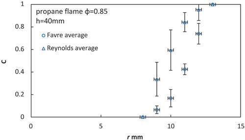
Figure 6 shows representative radial profiles of the Favre-averaged progress variable and the Reynolds-averaged progress variable . Both horizontal and vertical error bars are shown, the former identifying positioning errors related mainly to the size of the measurement volume and the latter reflecting the errors in estimating the progress variable as discussed above. The error bars in both directions represent estimated maximum errors. While the C = 0 and C = 1 positions are, of course, the same for both averages, the Reynolds average increases more steeply because of the absence of the density weighting. In addition, because of the weighting, the uncertainty in the Reynolds average increases with respect to the uncertainty in the Favre average as the value of the Favre average decreases. The 40-mm height was selected for this figure instead of the 50-mm height of Figure 2 because of the slight burned-gas flamelet contribution seen in the upper right-hand plot of Figure 2, which implies that C is not exactly zero there; the corresponding plot at 40 mm exhibits no burned-gas contribution.

Figure 6. Favre, , and Reynolds, , average progress variable at 40 mm height for the propane flame of ϕ = 0.85; the error bars here represent maximum possible errors and expected errors are about half of what is shown.

The error bounds in Figure 6 are typical of the bounds for all of the data. With that in mind, errors are not indicated for other cases. Figure 7 shows the best-guess radial profiles of Favre-averaged progress variables at different heights for all four flames. The curves for the three heights shown in the upper plot apply to both the lean and the rich methane flames, the differences between those two flames being much less than the experimental uncertainty. Concerning the propane flames in the lower graphs, only two heights are shown for the rich flame because that flame was too short to obtain data at the highest elevation; the average progress variable at any given radius for the rich propane flame is appreciably greater than that for the lean flame at the same height. Reynolds averages can be calculated from these Favre averages according to = /(1 + r (1 – )], where r = /.

Figure 7. Approximate radial distributions of Favre average progress variable.

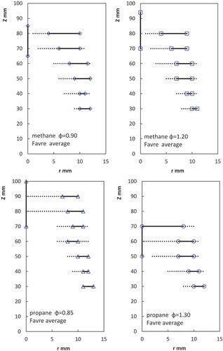
From results like those in Figure 6, contour plots of curves of constant values of average progress variables can be constructed in the radius-height (r-z) plane. Figure 8 shows such plots for all four flames for a Favre-averaged progress variable of 0.5. Such curves have the same general shape for other values of the Favre-averaged progress variable, as well, although the radius increases with increasing . Corresponding contours for constant values of the Reynolds-averaged progress variable have similar shapes. In this figure, solid horizontal lines with symbols at their ends bound the range of the data as previously described. The lengths of these solid lines generally increase with height because the clarity with which the bi-modality can be identified decreases as the flame-brush tip is approached, associated with an increasing range of radius over which two weak peaks may exist. The bounds, notably for the lean propane flame in the lower left-hand plot, strongly suggest that the contour achieves a minimum radius, in that case at a height of 60 mm. Above that there appears to be a kind of fresh-mixture average “bubble,” which closes rapidly at the top of the flame just below 100 mm in that case. Attempts to identify this from the photographs in Figure 1 were not successful. Although there is some uncertainty about this, it is of interest to call this possibility to the reader’s attention as discussed later.

Figure 8. Distribution map of possible zone of the progress variable based on Favre averaging and the zone in which the bi-modal distribution is observed of the methane flames (upper) and propane flames (lower), and the symbols bound the maximum possible range of the contour, the probable range being about half the range shown.

Since the bi-modality of the radial velocity distribution does not occur on the centerline, it is difficult to extend these contour plots to r = 0. Accurate centerline locations of the contours, therefore, are not available. The = 0.5 profiles on the centerline must lie somewhere within the turbulent flame brush there, and bounds of the brush can be identified with inflection points of centerline profiles of root-mean-square fluctuations of transverse velocities. These fluctuations abruptly begin to increase at a height where flamelets are first encountered, and they abruptly begin to decrease above a height at which flamelets are no longer present, as may be seen in the profiles shown in Figure 9. These two inflection-point heights are marked by symbols on the centerline in Figure 8. The lower of these two values is well below the position where = 0.5, but the upper value may lie very near = 0.5. These upper values support a very rapid closing of the “bubble.”

Figure 9. Axial distributions of the root mean square transverse component of velocity on the centerline.

The horizontal dotted lines in Figure 8 show the full range of radius over which bi-modal radial velocity distributions occur. This range affords one possible definition of the thickness of the turbulent flame brush. Approximate values of the resulting flame-brush thicknesses are plotted in Figure 10, where it is seen that they are indistinguishable within experimental error for the two methane flames, perhaps a little smaller at the lower heights for the lean propane flame, but clearly significantly larger for the rich propane flame. The outer radius of the bimodal region does not vary much with height, but the inner radius decreases rapidly with height, causing the turbulent-flame thickness to increase with height, nearly until the flame tip is reached. The more rapid increase for the rich propane flame is a further indication of the previously mentioned preferential-diffusion effect for this flame. While these results have been extracted from Favre-averaged data, essentially the same results (not shown) have also been obtained from Reynolds-averaged data. It must be realized that these thicknesses pertain to thicknesses measured in the radial direction, which except at the lowest heights are larger than thicknesses measured normal to the average flame brush. The latter also increases with height but is more difficult to extract as accurately from the present data. Smaller integral length scales near exit-tube edges would be consistent with smaller flame-brush thicknesses there.

Figure 10. Thickness of turbulent flame brush obtained from the progress variable of the methane (upper) and propane (lower) flames.

Conditioned and unconditioned average velocities and intensities

Modeling studies of turbulent combustion in the corrugated-flamelet regime often address velocity-component averages separately conditioned on the fresh mixture and the burned gas. For purposes of comparison, it therefore can be helpful to have experimental data on such conditioned averages. Such data can be generated for the radial component of velocity from the results given above. While it is clear that such conditioned averages cannot be obtained from the present measurements for the axial or tangential component of gas velocities, results for the radial component can afford useful tests. Corresponding conditioned means and conditioned intensities were therefore extracted from the radial component of the LDV data.

As previously discussed, overlap of the fresh-mixture and burned-gas distributions and contributions from data points within flamelets introduce uncertainties into the calculated results. One aspect of the data that has negligible uncertainty is the value of the velocity at each of the two peaks of the bi-modal distribution, which is likely to be an excellent measure of the true mode of the respective conditioned distribution, since the overlaps and flamelet-interior contributions are not likely to have strong influences on these modes. If the fresh-mixture or burned-gas distribution is symmetric, then the corresponding peak coincides with the conditioned average. If, however, one of the distributions is symmetric, then the other may not be. It is therefore desirable to attempt to estimate the maximum possible effect of a departure from symmetry on the value of the conditioned mean.

Although there is no foolproof way to estimate effects of departures from symmetry, an indication of the magnitude of such an effect can be obtained from the conditioned means calculated on the assumption that the minimum point in the distribution between the two peaks divides the fresh mixture on the left from the burned gas on the right. For most of the data points, this assumption results in decidedly non-symmetrical distributions. When such conditioned averages were computed, however, they always were found to be very close to the velocities at the two peaks of the distribution. Therefore, possible asymmetries in the distributions seem likely to have little influence on the conditioned means. In this respect, the uncertainties in values of the conditioned means appear to be considerably less than those in values of the average progress variable.

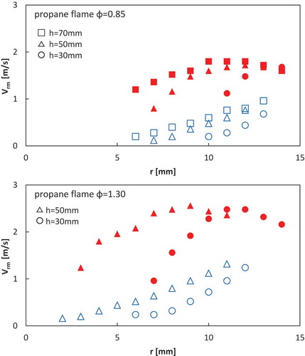
Figure 11 shows radial profiles of the most probable radial component of velocity in the fresh mixture and in the burned gas at three different heights in the lean methane flames. Within experimental error, the corresponding results for the rich methane flame are identical. Moreover, it is seen that the velocities for the burned gas are much larger than those for the unburned gas and that both increase with increasing radius and height. The upper and lower graphs in Figure 12 show these same results for the lean and rich propane flames, respectively. Comparison of Figures 11 and 12 demonstrate that the results are appreciably different for the rich and lean propane flames in that the conditioned radial velocities at any given height in the lean propane flame are noticeably lower than those at the same height in the methane flames, while the profiles at a given height in the rich propane flame are appreciably higher than those in the methane flames. Thus, there are differences in the propane flames that are not present in the methane flames.

Figure 11. Comparison of radial distribution of conditioned most probable radial component of velocity for the methane flame of ϕ = 0.9 at 30-mm, 50-mm, and 70-mm heights; open symbols are fresh mixture, solid symbols are burned gas.

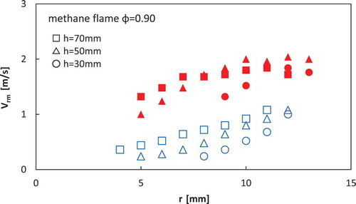
Figure 12. Comparison of radial distribution of conditioned most probable radial component of velocity for the propane flames of ϕ = 0.85 (upper) and 1.30 (lower) at 30-mm, 50-mm, and 70-mm heights; open symbols are fresh mixture, solid symbols are burned gas.

Favre-averaged radial components of velocity are readily computed from these conditional averages. Their variations with radius and height are similar to those of the conditioned quantities, as may be seen in Figure 13 for the methane flames and in the upper and lower graphs of Figure 14 for the lean and rich propane flames, respectively. The general increase with radius, seen here for the average radial component of velocity, is not found for the average axial component of velocity (not shown), which remains fairly independent of the radius. It does, however, increase with increasing height, up to the tip of the turbulent flame brush, as can be seen in the centerline averages shown in Figure 15 for all four flames. The curve for the rich methane flame is similar to that of the corresponding lean flame, although its velocity levels appear to be slightly lower at the lower heights and higher at the higher heights, perhaps suggesting influences of the outer diffusion flame in the former case in need of further study. The rich propane flame is seen here to be much shorter than the lean propane flame as indicated previously.

Figure 13. Radial distribution of Favre averaged radial component of velocity for the methane flame of ϕ = 0.9 at 30-mm, 50-mm, and 70-mm heights.

Figure 14. Radial distribution of Favre averaged radial component of velocity for the propane flames of ϕ = 0.85 (upper) and 1.30 (lower) at 30-mm, 50-mm, and 70-mm heights.

Figure 15. Axial distribution of Favre averaged axial component of velocity on the centerline for the four flames.

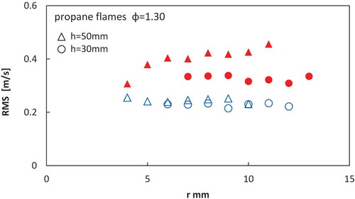
Conditioned root-mean-square fluctuations of radial components of velocity can be computed in the same manner as the conditional averages. Radial profiles of these conditional intensities at three different heights are shown in Figure 16 for the lean methane flame, which agree with those for the rich methane flame within experimental error. Although these plots may appear to suggest a decrease in the fluctuation intensity of the fresh mixture with increasing radius, that is an artifact of the procedure employed in calculating the conditioned averages; as the radius increases, an increasing fraction of the data points are in the burned gas, causing the minimum point of the distribution to move into the region of the distribution of the fresh mixture, thereby excluding fresh-mixture points that, if included, would produce higher intensities. The fresh-mixture values therefore are independent of the radius within the accuracy of the computations, but the burned-gas intensities do increase detectibly with radius within the accuracy. In addition, there is no apparent variation of the fresh-mixture values with height, while the burned-gas values clearly increase with height. The overall Favre-averaged intensity will increase with radius and height, somewhat like the intensity conditioned on the burned gas. While the conditioned intensity distributions are essentially the same for the two methane flames, they are appreciably different for the two propane flames, with the rich propane flame exhibiting significantly higher intensities, as can be seen by comparing Figures 17 and 18.

Figure 16. Comparison of radial distribution of conditioned root-mean-square fluctuations of radial components of velocity for the methane flame of ϕ = 0.9 at 30-mm, 50-mm, and 70-mm heights; open symbols are fresh mixture, solid symbols are burned gas.

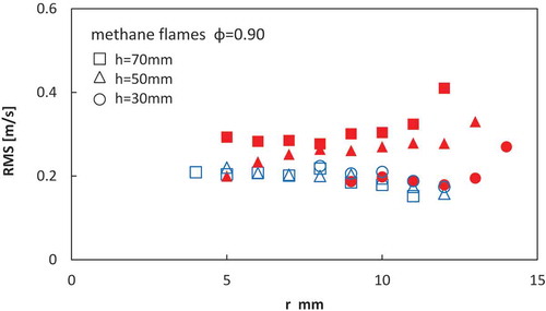
Figure 17. Comparison of radial distributions of conditioned root-mean-square fluctuations of radial components of velocity for the propane flame of ϕ = 0.85 at 30-mm, 50-mm, and 70-mm heights; open symbols are fresh mixture, solid symbols are burned gas.

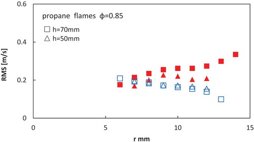
Figure 18. Comparison of radial distributions of conditioned root-mean-square fluctuations of radial components of velocity for the methane flame of ϕ = 1.30 at 30-mm, 50-mm, and 70-mm heights; open symbols are fresh mixture, solid symbols are burned gas.

Turbulent burning velocities

Although there are a variety of different definitions of turbulent burning velocities, it is of interest to investigate values of this quantity that may be obtained from the present results. Statistically homogeneous conditions in directions transverse to the direction of propagation of turbulent flames are difficult to establish experimentally, and the Bunsen flame is not an exception. Average orientations of flamelets with respect to the mean flow direction, for example, will be different in the lower part of the flame brush than in the upper part, and corresponding differences may be expected in local turbulent burning velocities. There is no evident direct way to extract local turbulent burning velocities from the present results. Overall averages may, however, be estimated as described below.

Kobayashi et al. (1996, 1998) applied the flame-angle method to superimposed Schlieren photographs of turbulent premixed flames to measure the turbulent burning velocities for Bunsen flames. Their experimental observations suggest that the results for the flame-angle turbulent burning velocity may apply over much of the central portion of the turbulent flame. The resulting burning velocities may, however, be different from values of burning velocities calculated from measured iso-contours of progress variables by a flame-area method, contours for which information was not available in their experiments. Since that information is available in Figure 8, for example, it may be of interest to calculate flame-brush average turbulent burning velocities from the mean-progress-variable results shown in that figure.

When burning velocities are calculated by the flame-area method from mean progress-variable iso-contours, the results depend on the value selected for the mean. A small mean value would apply to the leading edge of the turbulent flame, while a mean value near unity would apply to the trailing edge. The former turbulent burning velocity would be larger, while the latter would be smaller in this configuration. It was suggested (Kobayashi et al., 1996) that the flame-angle measurements were likely to correspond most nearly to a Reynolds-averaged progress variable of = 0.5, and based on earlier measurements (Smallwood et al., 1995), the turbulent-flame area at this value was estimated to be 1.2 to 1.5 times that at = 0.05, this latter value having been suggested (Smallwood et al., 1995) to be a reasonable representation of the leading edge of the turbulent flame. Recent modeling efforts (Kolla et al., 2009, 2010; Kolla and Swaminathan, 2011) have focused on the motion of this leading edge, which therefore would be a desirable value to select.

With the present data, however, the values of the burning velocities at small values of the average progress variable would be very uncertain because of the large uncertainty in the associated area, especially in the important near-centerline region. Because variations of turbulent-flame areas with may be expected to depend appreciably on such experimental conditions as fresh-mixture flow rates, it could be dangerous to employ earlier results (Smallwood et al., 1995) to estimate the area-ratio variation associated with the mean-flow expansion. For that reason, no attempt is made here to address the leading-edge turbulent-flame propagation velocity, the flame-angle burning velocity, or any of the various other possible definitions. Instead, velocities are calculated only by considering a value of for which results can be obtained most accurately from the present data. Even with this restriction, significant uncertainty remains.

In view of these considerations, the contour for which the Reynolds-averaged progress variable is = 0.5 was selected for calculation. This provides an intermediate value for the turbulent burning velocity, which will be somewhat greater than the value that would have been obtained if this midpoint value of the Favre average had been chosen instead. The Reynolds average was employed because density weighting should not be relevant to determining the average position of the mean surface. The flame-area of this iso-contour is an average flame-area from which the burning velocity is calculated from the equation , where is the flow rate of the mixture at the burner exit. The specific procedure employed was to select the most probable Reynolds-averaged 0.5 contours similar to those shown in Figure 8, approximate them by three straight lines beginning vertically at the exit and ending horizontally at the centerline, and then computing the axisymmetric area of the resulting construction. In view of uncertainties in area determinations and possible variations associated with heating of the incoming mixture by the heated tube walls, results for turbulent burning velocities can be extracted at best to just one significant figure.

With this procedure, the turbulent burning velocities are found to be 0.8 m/s for both methane flames, 0.6 m/s for the lean propane flame, and 1.0 m/s for the rich propane flame. Thus, even though the experiments have been conducted with identical characteristics of the turbulence and with the same laminar burning velocity, the turbulent burning velocity of the rich propane flame is seen to be much larger than that of the lean propane flame and, in addition, while the turbulent burning velocity of the rich propane flame exceeds that of the methane flames, the turbulent burning velocity of the lean propane flame is less than that of the methane flames.

Effects of differential diffusion

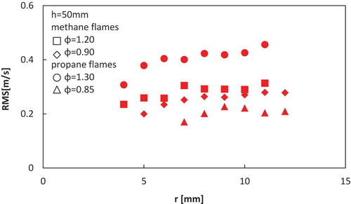
Further clarification of possible effects of differential-diffusion phenomenon can be seen by comparing the burned-gas results shown in Figures 11 and 12 at the same heights for all four flames. The data in Figure 19 exhibits a comparison of radial profiles of burned-gas conditioned average radial components of gas velocity for all four flames at 50 mm above the exit plane where, according to Figure 8, all four of the turbulent flame brushes are reasonably well developed. As explained previously, these conditioned averages are more uncertain than the most-probable distributions shown in Figures 11 and 12, but they are not very different from them. It is seen in Figure 19 that, while the data for the rich and lean methane flames are essentially the same, not only are the burned-gas conditioned radial velocity components for the rich propane flame higher than those for the methane flames, but also the same conditioned values for the lean propane flame are appreciably lower than those of the methane flames. This same relative ordering also applies to the burned-gas conditioned root-mean-square radial-velocity fluctuations, as can be seen in Figure 20.

Figure 19. Radial distribution of average value of the radial component of the burned gas velocity for the four flames at 50-mm height.

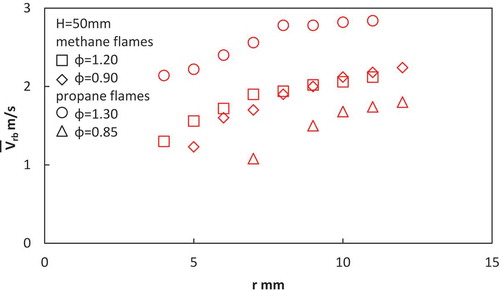
Figure 20. Radial distribution of the root mean square of the radial component of the burned gas velocity for the four flames at 50-mm height.

As indicated in the introduction, in earlier work (Furukawa et al., 2010) on the basis of measurements of flamelet motions, we identified clear differences between the turbulent flame structures of rich and lean propane flames hypothesizing that the differences arise from turbulence-produced flamelet wrinkling, followed by preferential oxygen diffusion to protruding wrinkles, thereby enhancing the average flamelet propagation velocity. The present gas-velocity measurements support this interpretation by demonstrating that the motions of the gas (as well as the flamelets) exhibit definite differences that are consistent with such differential-diffusion effects. Moreover, the rich and lean propane flames exhibit gas-motion differences of roughly equal magnitudes but in opposite directions, compared with gas motions in corresponding methane flames. The structural differences between the methane flames and the propane flames were not addressed in the previous discussion of flamelet-motion measurements (Furukawa et al., 2010) where the emphasis on effects of equivalence ratio was focused on propane, but they can be seen by comparing the plots of the probability distributions for magnitudes of flamelet velocities shown in Figure 26 with the corresponding propane results shown in Figure 29 of that paper.

These differences do, however, appear to be consistent, at least indirectly, with results of certain investigations employing direct numerical simulation (DNS). In particular, computations of Haworth and Poinsot (1992) indicated clearly that, for non-unity Lewis numbers, local consumption speeds in turbulent premixed flames are more correlated with curvature than with strain rate, contrary to flames with Lewis numbers of unity. Recent DNS results (Nikolaou et al., 2014) employing both skeletal and reduced chemistry for a stoichiometric synthetic fuel mixture in the thin-reaction-zone regime also produced stronger correlations with curvature than with strain rate. These conclusions are also supported by other DNS results (Poinsot and Veynante, 2001). Although the first computation (Haworth and Poinsot, 1992) was restricted to single-reactant flames, the finding that more flame area was generated for Lewis numbers less than unity and less for Lewis numbers greater than unity is consistent with the idea that in two-reactant flames when the deficient reactant has a higher diffusion coefficient it will diffuse preferentially to turbulence-generated wrinkles, thereby increasing the local burning velocity there with a resulting positive increment in the turbulent burning velocity, while if the deficient reactant has a lower diffusion coefficient, its diffusion to a wrinkle is preferentially retarded, thereby decreasing the local burning velocity and contribution of a negative increment to the turbulent burning velocity. The comparatively few existing theoretical analyses of two-reactant flames (Matalon et al., 2003) have not yet progressed to addressing these turbulent-flow effects, nor has other literature on turbulent combustion (Driscoll, 2008; Lipantnikov and Chomiak, 2005) identified this specific phenomenon.

Consideration of the mechanism involved readily yields scaling estimates of associated corrections to turbulent burning velocities. The differential diffusion alters the flamelet stoichiometry locally, thereby changing the rate of heat release in the reaction zone at a wrinkle protruding into the fresh mixture. The magnitude of the resulting fractional change in the turbulent burning velocity, compared with that of a stoichiometric mixture, may be expected to be roughly proportional to a factor f, defined as the difference between the maximum laminar burning velocity and the laminar burning velocity of the fresh mixture, S_L, divided by S_L. Letting D denote the difference between the diffusion coefficients of the deficient and abundant reactants, the change in the turbulent burning velocity must also be proportional to D/l, where l is a representative radius of curvature of a wrinkled flamelet. The value of l should be on the order of the integral scale L of the turbulence in the approach flow, so long as S_L is not too large compared with the root-mean-square turbulent fluctuation velocity u′ of the fresh mixture. Since laminar flame propagation through turbulent eddies reduces flamelet curvature, a final approximation to the fractional change of the turbulent burning velocity can be suggested to be f(D/L) exp(–S_L/u′). In this suggestion, D carries the flamelet effect, while L and the exponential factor carry the turbulence effect.

Although eddies of all sizes, in principle, can participate in this phenomenon, to the extent that Kolmogorov scaling and the exponential correction factor apply, the largest eddies should dominate because of the exponential falloff for smaller eddies. While similar local preferential-diffusion phenomena would be anticipated for stretched flamelets, if they remain planar then effects of regions of high and low strain rates may be expected to tend to cancel, exerting at most small influences on turbulent burning velocities, unlike these curvature effects, for which diffusion to leading points should modify turbulent burning velocities more strongly. Considerations of different planar flamelet structures for rich and lean conditions without invoking preferential diffusion failed to explain the observations. It should be emphasized that the preceding formula is only a suggestion and that more thorough mechanistic modeling investigations are called for, the thrust of the present contribution being experimental rather than modeling.

This result indicates that the differential diffusion phenomenon encountered here thus should scale with a fractional difference in laminar burning velocities with a difference in the diffusion coefficients of the deficient and abundant components and with the reciprocal of the integral scale of the turbulence, exhibiting an attenuation factor dependent on the ratio of the laminar burning velocity to the fluctuation velocity of the turbulence and related to the Gibson scale. The heat-release rates, wrinkling, and flamelet-surface-area increases are enhanced when the diffusion-coefficient difference is positive (the deficient reactant has the larger diffusion coefficient), and they are reduced when this difference is negative (the deficient reactant has the smaller diffusion coefficient). Small-scale, high-intensity turbulence, so long as it is still in the corrugated-flamelet regime, would favor this mechanism becoming important according to the scaling formula proposed here. Quantitative estimates of the magnitude of the effect would require much more detailed work in turbulent-combustion modeling, with the specific details differing, for example, for different types of LES. The flamelet effect could be studied on the basis of a Markstein number for curvature and then incorporated in flamelet sub-grid models. On the other hand, with sub-grid G-equation modeling preferential-diffusion corrections to turbulent burning velocities would arise, but as a first approach in flamelet modeling at the sub-grid level, it may be sufficient simply to revise the equivalence ratio of the selected flamelets.

Discussion of results

One discovery of the present measurements is the “bubble” mentioned previously. Despite aforementioned uncertainties, it is supported most clearly by the lower left graph of Figure 8, but there certainly is no indication of it in Figure 1. This shows that different methods of measurement can produce qualitatively different ideas concerning turbulent flame structures. The experimental methods of Kobayashi et al. (1997) reveal what appear to be flapping flamelets that could be responsible for the development of the “bubble” at the top of the turbulent flame brush in the progress-variable iso-contours of the Bunsen flame. This phenomenon has not been found in turbulent-flame modeling and it would be of interest to investigate what types of modeling assumptions might lead to prediction of such a phenomenon.

Another result is the new support for differences between the turbulent flame structure of the rich and lean propane flames and the corresponding methane flames documented perhaps most clearly in Figure 19, which in our opinion now renders that conclusion well-established experimentally. Hypothesized in an earlier paper for the rich propane flame, on the basis of measurements of flamelet motion, the present work verifies the existence of this phenomenon through measurements of gas velocities, as well as revealing a related difference for the lean propane flame. Apparently consistent with the few available relevant DNS results, this effect too is not present in current modeling of premixed turbulent flames in the corrugated-flamelet regime. An approach to taking account of this phenomenon in modeling efforts is suggested above, but further research in turbulent-combustion modeling is warranted, both for addressing these differences as well as describing the structures measured here. It could be associated with the onset of shear-layer interactions of the turbulent flame with the outside air, and it may become more pronounced at higher flow rates, as the flame becomes taller.

It is surprising that the bi-modal distribution of the radial component of the gas velocity, seen in Figures 2 and 5, has not been reported previously for turbulent Bunsen flames. The interpretation of this observation, in terms of measurement positions being predominantly located in the fresh mixture or in the burned gas, enables good estimates to be made of the progress-variable fields in this flamelet regime. It is on the basis of such estimates that effects of preferential diffusion on turbulent flame structures can be identified most clearly, such as the associated differences in the thickness of the turbulent flame brush shown in Figure 10 and in the turbulent burning velocities indicated in the text. Also, in this way conditioned statistics, such as the results shown in Figures 11, 12, and 16–20, can be extracted from the data, which in the future may be compared with future modeling predictions. The bimodality thus uncovers many aspects of turbulent Bunsen-flame structures that are not at all evident in other approaches to measurement and observation, such as the photographs seen in Figure 1.

Various differences between rich and lean premixed turbulent propane Bunsen flames having the same laminar burning velocities not reflected in corresponding methane flames, based on the new experimental results shown in Figures 5, 7, 9, 10, 12, 14, 15, 19, and 20, have been explained here on the basis of different rates of diffusion of propane and oxygen to turbulence-generated flamelet bulges pointing into the fresh mixture and an approach to modeling that effect was initiated. The absence of the effect for methane flames, because of the close similarity of the diffusion coefficients of methane and oxygen, is consistent with the explanation that has been offered. Since there are no other evident differences between these two hydrocarbon flames that can explain such kinds of observations, differential-diffusion phenomena deserve further consideration for the corrugated-flamelet regime.

Conclusions

It may be concluded from this study that LDV measurements are capable of revealing a number of aspects of the structures of turbulent Bunsen flames in the corrugated-flamelet regime. Through flapping motions of predominantly nearly vertical flamelet sheets in this regime, non-monotonic variations of mean reaction progress variables with increasing height at a fixed radius appear to develop for sufficiently tall turbulent flames, likely increasing with increasing reactant flow rates but not discernable in our photographs of the flames. Equidiffusional mixtures in this regime exhibit essentially identical turbulent flame structures for rich and lean flames having the same laminar burning velocity. The turbulent flame structures, however, are different for rich and lean mixtures having the same laminar burning velocity if the diffusion coefficient of the fuel is appreciably less than that of the oxygen and diluent. In that case, through preferential diffusion of oxygen to turbulence-induced flamelet bulges extending towards the fresh mixture, the rich mixture develops higher average flamelet propagation velocities and greater flamelet areas, which lead to greater turbulent burning velocities and turbulent flame-brush thicknesses than those of the corresponding lean mixture. In addition, for this lean mixture, the slower rate of fuel diffusion to such bulges reduces the average flamelet propagation velocities and flamelet areas compared with those of the corresponding equidiffusional mixtures, thereby leading to smaller turbulent burning velocities and flame-brush thicknesses. Thus, preferential diffusion, in general, exerts measurable influences on turbulent flame structures in the corrugated flamelet regime.

Acknowledgments

We would especially like to thank N. Swaminathan for helpful comments. N. Chakraborty and D. Haworth identified helpful literature.

Funding

The contribution of the third author was supported by the US AFOSR Grant #FA9550-12-1-0138.

Additional information

Funding

The contribution of the third author was supported by the US AFOSR Grant #FA9550-12-1-0138.

References

- Bilger, R.W. 2000. Future progress in turbulent combustion research. Prog. Energy Combust. Sci., 26, 367–380.
- Bollinger, L.M., and Williams, D.T. 1949. Effect of Reynolds number in turbulent-flow range on flame speed of Bunsen burner flames. NACA Report 932.
- Chen, Y.C., and Bilger, R.W. 2001. Simultaneous 2-D imaging measurements of reaction progress variable and OH radical concentration in turbulent premixed flames: Experimental methods for flame brush structure. Combust. Sci. Technol., 167, 131–167.
- Chen, Y.C., and Bilger, R.W. 2002. Experimental investigation of three-dimensional flame-front structure in premixed turbulent combustion—I: Hydrocarbon/air bunsen flames. Combust. Flame, 131, 400–435.
- Chakraborty, N., Katragadda, M., and Cant, R.S. 2011a. Statistics and modelling of turbulent kinetic energy transport in different regimes of premixed combustion. Flow Turbul. Combust., 87, 205–235.
- Chakraborty, N., Katragadda, M., and Cant, R.S. 2011b. Effects of Lewis number on turbulent kinetic energy transport in premixed flames. Phys. Fluids, 23, 075109.
- Driscoll, J.F. 2008. Turbulent premixed combustion: Flamelet structure and its effect on turbulent burning velocities. Prog. Energy Combust. Sci., 34, 91–134.
- Frank, J.H., Kalt, P.A.M., and Bilger, R.W. 1999. Measurement of conditional velocities in turbulent premixed flames by simultaneous OH PLIF and PIV. Combust. Flame, 116, 220–232.
- Furukawa, J., Hashimoto, H., and Williams, F.A. 2010. Flamelet motion in premixed turbulent axisymmetric rod-stabilized and Bunsen flames. Combust. Sci. Technol., 182, 1–38.
- Furukawa, J., Maruta, K., and Hirano, T. 1998. Flame front configuration of turbulent premixed flames. Combust. Flame, 112, 293–301.
- Furukawa, J., Nakamura, T., and Hirano, T. 1994. Electrostatic probe measurement to explore local configuration of a high intensity turbulent premixed flames. Combust. Sci. Technol., 96, 169–181.
- Furukawa, J., Noguchi, Y., Hirano, T., and Williams, F.A. 2002. Anisotropic enhancement of turbulence in large-scale, low-intensity turbulent premixed flames. J. Fluid Mech., 462, 209–243.
- Furukawa, J., and Williams, F.A. 2003. Flamelet effects on local flow in turbulent premixed Bunsen flames. Combust. Sci. Technol., 175, 1835–1858.
- Furukawa, J., Yoshida, Y., Amin, V., and Williams, F.A. 2013a. Changes of gas velocities in passing through flamelets in a premixed turbulent Bunsen flame. Combust. Sci. Technol., 185, 200–211.
- Furukawa, J., Yoshida, Y., and Williams, F.A. 2013b. Evolution of gas velocities behind flamelets in a premixed turbulent Bunsen flame. Combust. Sci. Technol., 185, 661–671.
- Haworth, D., and Poinsot, T. 1992. Numerical simulation of Lewis number effects in turbulent premixed flames. J. Fluid Mech., 244, 405–436.
- Hottel, H.C., Williams, G.C., and Levine, R.S. 1953. The influence of isotropic turbulence on flame propagation. Proc. Combust. Inst., 4, 636–644.
- Jones, W.P. 1994. Turbulence modeling and numerical solution methods for variable density and combusting flows. In P.A. Libby and F.A. Williams (Eds.), Turbulent Reacting Flows, Academic Press, London, pp. 309–374.
- Karlovitz, B., Denniston, Jr., D.W., Knapsachaefer, D.H., and Wells, F.E. 1953. Studies of turbulent flames. A. Flame propagation across velocity gradients. B. turbulence measurements in flames. Proc. Combust. Inst., 4, 613–620.
- Kobayashi, H., Kawabata, Y., and Maruta, K. 1998. Experimental study on general correlation of turbulent burning velocity as high pressure. Proc. Combust. Inst., 27, 941–948.
- Kobayashi, H., Nakashima, T., Tamura, T., Maruta, K., and Niioka, T. 1997. Turbulence measurements and observations of turbulent premixed flames at elevated pressures up to 3.0 MPa. Combust. Flame, 108, 104–117.
- Kobayashi, H., Tamura, T., Maruta, K., Niioka, T., and Williams, F.A. 1996. Burning velocity of turbulent premixed flames in a high-pressure environment. Proc. Combust. Inst., 26, 389–396.
- Kolla, H., Rogerson, J.W., Chakraborty, N., and Swaminathan, N. 2009. Scalar dissipation rate modeling and its validation. Combust. Sci. Technol., 181, 518–535.
- Kolla, H., Rogerson, J.W., and Swaminathan, N. 2010. Validation of a turbulent flame speed model across combustion regimes. Combust. Sci. Technol., 182, 284–308.
- Kolla, H., and Swaminathan, N. 2011. Influence of turbulent scalar mixing physics on premixed flame propagation. J. Combust., 8, 451351.
- Libby, P.A., and Williams, F.A. 1980. Turbulent Reacting Flows, Springer-Verlag, Berlin, 243 pp.
- Libby, P.A., and Williams F.A. 1994. Turbulent Reacting Flows, Academic Press, London, 303 pp.
- Lipatnikov, A.N., and Chomiak, J. 2005. Molecular transport effects on turbulent flame propagation and structure. Prog. Energy Combust. Sci., 31, 1–73.
- Matalon, M., Cui, C., and Bechtold, J.K. 2003. Hydrodynamic theory of premixed flames: Effects of stoichiometry, variable transport coefficients and arbitrary reaction orders. J. Fluid Mech., 487, 179–210.
- Nikolaou, Z.M., Swaminathan, N., and Chen, J.Y. 2014. Evaluation of a reduced mechanism for turbulent premixed combustion. Combust. Flame, 161, 3085–3099.
- Peters, N. 2000. Turbulent Combustion, Cambridge University Press, Cambridge, UK, pp. 66–169.
- Pfadler, S., Kerl, J., Beyrau, F., Leipertz, A., Sadiki, A., Scheuerlein, J., and Dinkelcaker, F. 2009. Direct evaluation of the subgrid scale scalar flux in turbulent premixed flames with conditioned dual-plane stereo PIV. Proc. Combust. Inst., 32, 1723–1730.
- Poinsot, T., and Veynante, D. 2001. Theoretical and Numerical Combustion, R. T. Edwards, Philadelphia, PA, pp. 252–267.
- Smallwood, G.J., Gülder, O.L., Snelling, D.R., Deschamps, B.M., and Gökalp, I. 1995. Characterization of flame front surfaces in turbulent premixed methane/air combustion. Combust. Flame, 101, 461–470.
- Steinberg, A.M., Driscol, J.F., and Ceccio, S.L. 2009. Temporal evolution of flame stretch due to turbulence and the hydrodynamic instability. Proc. Combust. Inst., 32, 1713–1721.
- Vagelopoulos, C.M., and Egolfopoulos, F.N. 1998. Direct experimental determination of laminar flame speed. Proc. Combust. Inst., 27, 513–519.
- Zhang, S., and Rutland, C.J. 1995. Premixed flame effects on turbulence and pressure-related terms. Combust. Flame, 102, 447–461.