Modeling of Progress Variable Variance Transport in Head-On Quenching of Turbulent Premixed Flames: A Direct Numerical Simulation Analysis

ABSTRACT

The statistical behavior of the transport of reaction progress variable variance has been analyzed using three-dimensional direct numerical simulation (DNS) data for different values of Damköhler, Karlovitz, and global Lewis numbers in the context of head-on quenching of turbulent premixed flames by an inert isothermal wall. It has been found that reaction rate contribution to the variance transport acts as a leading order source, whereas the molecular dissipation term remains as the leading order sink for all cases considered here. However, all of the terms of the variance transport equation decay significantly in the near-wall region once the quenching starts. The existing models for the turbulent transport, reaction, and dissipation contributions to the variance transport do not adequately capture the near-wall behavior. The wall effects on the unclosed terms of the variance transport equation have been analyzed using explicitly Reynolds averaged DNS data and the existing closures of the unclosed terms have been modified to account for the near-wall effects. A-priori DNS analysis suggests that the proposed modifications to the existing closures for the unclosed terms of the variance transport equation provide satisfactory predictions both away from and near to the wall.

KEYWORDS:

• Direct numerical simulation (DNS)
• Flame wall interaction
• Head-on quenching
• Lewis number
• Progress variable variance
• Reynolds averaged Navier–Stokes simulation

Introduction

The variance of reaction progress variable plays a pivotal role in the modeling of turbulent premixed combustion (Bray, 1980; Swaminathan and Bray, 2011). The magnitude of the variance of reaction progress variable is often necessary for the modeling of mean reaction rate in the context of Reynolds Averaged Navier–Stokes (RANS) simulations (Bray et al., 2006; Linstedt and Vaos, 1999; Mantel and Bilger, 1995; Moler et al., 1996; Mura et al., 2007; Ribert et al., 2005; Robin et al., 2006). The reaction progress variable c can be defined in terms of a suitable reactant mass fraction Y_R in the following manner:

(1)

According to Eq. (1), increases monotonically from zero in the unburned gas (subscript 0) to unity in fully burned products (subscript ). The variance of reaction progress variable is given by: , where and represent the Favre average and Favre fluctuation of a general quantity q, respectively, with being the gas density, and the Reynolds averaging is shown by the overbar. The scalar variance is one of the important quantities for the flamelet (Bray et al., 1985; Linstedt and Vaos, 1999; Swaminathan and Bray, 2011) and conditional moment (Klimenko and Bilger, 1999; Swaminathan and Bilger, 2001) based closures. Consequently, the variance is often required for the well-known eddy break up (EBU) models (Linstedt and Vaos, 1999; Swaminathan and Bray, 2005). Furthermore, is an essential gradient of the tabulated chemistry based modeling of turbulent premixed combustion (Domingo et al., 2005; Savre et al., 2008).

Based on a presumed bi-modal probability density function (pdf) of with impulses at and according to the Bray–Moss–Libby (BML) model (Bray et al., 1985), one obtains:

(2)

where is the burning mode contribution. The contribution of can be neglected and assumes its maximum possible value when can be approximated by a bi-modal distribution with impulses at and , and this condition is realized for high values of Damköhler number (i.e., ), where the flame front is thinner than the Kolmogorov length scale, and the turbulent eddies do not affect the flame structure. However, cannot be neglected for small values of (i.e., ) and subsequently remains smaller than , and thus, it is necessary to solve variance transport equation along with other modeled conservation equations in the context of RANS simulations. Chakraborty and Swaminathan (2011) and Malkeson and Chakraborty (2010) analyzed the statistical behaviors of scalar variance transport in turbulent premixed and stratified flames, respectively. Furthermore, Chakraborty and Swaminathan (2011) demonstrated that global Lewis number has significant influences on the various terms of the transport equation of . However, all of the aforementioned analyses have been carried out for flames, which are away from the wall, and the analysis of reaction progress variable variance transport in the near-wall region during flame-wall interaction is yet to be addressed in existing literature. A number of previous studies (Alshaalan and Rutland, 1998, 2002; Bruneaux et al., 1996, 1997; Dabireau et al., 2003; Gruber et al., 2010, 2012; Lai and Chakraborty, 2015; Poinsot et al., 1993) analyzed flame-wall interaction using three-dimensional (3D) DNS data. Poinsot et al. (1993) discussed about possible wall functions in the context of flame surface density (FSD)-based closure using 2D DNS data of head-on quenching of turbulent premixed flames. Bruneaux et al. (1997) proposed near-wall modifications to the models of the unclosed terms of the FSD transport equation based on channel flow DNS data. Alshaalan and Rutland (1998, 2002) addressed the near-wall closure of FSD and turbulent scalar flux for turbulent premixed flame-wall interaction. Dabireau et al. (2003) analyzed the statistical behavior of wall heat flux for both premixed and diffusion flames based on DNS data. Gruber et al. (2010, 2012) carried out 3D detailed chemistry DNS of turbulent premixed flame interaction with an inert isothermal wall and indicated the presence of flame instabilities, which are yet to be understood in detail. Recently, Lai and Chakraborty (2015) have proposed near-wall modifications to a well-known scalar dissipation rate (SDR)-based mean reaction rate closure proposed by Bray (1980) and also extended an algebraic SDR closure for accurate prediction of the near-wall behavior using DNS data of head-on quenching of statistically planar turbulent premixed flames by an isothermal inert wall. Lai and Chakraborty (2015) also analyzed the effects of global Lewis number on the statistical behaviors of wall heat flux, flame quenching distance, and the closures of SDR and mean reaction rate in the context of head-on quenching of turbulent premixed flames. It is worth noting that none of the aforementioned analyses on flame-wall interaction concentrated on the statistical behavior of the variance transport in the near-wall region. In order to address this gap in existing literature, the present analysis concentrates on the analysis of the variance transport in the near-wall region for head-on quenching of statistically planar turbulent premixed flames with global Lewis number ranging from 0.8–1.2 for different normalized values of root-mean-square turbulent velocity and integral length scale , where , , , , , and are the unstrained laminar burning velocity, thermal flame thickness, thermal diffusivity, thermal conductivity, specific heat at constant pressure, and mass diffusivity, respectively. Thus, the main objectives of the current analysis are:

1. To identify the near-wall effects on the statistical behavior of the unclosed terms of the scalar variance transport equation.

2. To propose modifications to the existing models of the unclosed terms of the variance transport equation in order to account for the near-wall behavior.

The rest of the article will be organized as follows. The information related to mathematical background and numerical implementation will be provided in the next two sections. Following this, results will be presented and subsequently discussed. The main findings will be summarized and main conclusions will be drawn in the final section of this article.

Mathematical background

The present analysis considers a single-step Arrhenius-type irreversible chemical reaction (i.e., ) for the purpose of computational economy as 3D DNS simulations with detailed chemistry remain prohibitively expensive for a detailed parametric analysis (Chen et al., 2009). An actual combustion process includes a number of species with different values of , but often the Lewis number of the deficient reactant is considered to be the characteristic Lewis number (Im and Chen, 2002; Mizomoto et al., 1984). Law and Kwon (2004) proposed a method for estimating the effective Lewis number based on heat release rate measurements, whereas Dinkelacker et al. (2011) proposed a methodology of estimating effective Lewis number as a linear combination the mole fractions of the mixture constituents. It is worth noting that several previous analyses (Clavin and Williams, 1982; Han and Huh, 2008; Haworth and Poinsot, 1992; Libby et al., 1983; Rutland and Trouvé, 1993; Sivashinsky, 1977; Trouvé and Poinsot, 1994) analyzed the effects of in isolation based on simple chemistry and the same approach has been adopted here. The instantaneous transport of reaction progress variable is governed by:

(3)

where is the reaction rate of reaction progress variable . Reynolds averaging of Eq. (3) yields:

(4)

The transport equation of the reaction progress variable variance can be obtained using relation :

(5)

where is the SDR of the reaction progress variable. In Eq. (5), is a closed term which denotes the molecular diffusion of . The term is the turbulent transport term, whereas denotes the generation/destruction of by the mean scalar gradient. The term is the reaction rate contribution and is the molecular dissipation term. The terms , and are the unclosed term in the context of transport. Equation (5) indicates that closure translates to the modeling of SDR . The modeling of , , , and in head-on quenching of turbulent premixed flames has been addressed here using explicitly Reynolds averaged 3D DNS data.

Numerical implementation

The conservation equations of mass, momentum, internal energy, and reaction progress variable for compressible reacting flows are solved in nondimensional form in the present analysis using a well-known DNS code SENGA (Jenkins and Cant, 1999). The simulation domain is taken to be a rectangular box of size , where is Zel’dovich flame thickness with and being the thermal diffusivity of the unburned gas and unstrained laminar burning velocity, respectively. The simulation domain is discretized using a Cartesian grid of ensuring 10 grid points across the thermal flame thickness , where , , and are the adiabatic flame temperature, unburned gas temperature, and the instantaneous dimensional temperature, respectively, and the subscript ‘L’ is used to refer to unstrained planar laminar flame quantities. A 10th-order central difference scheme has been used for the spatial discretisation for the internal grid points and the order of differentiation gradually drops to a one-sided 2nd-order scheme at the nonperiodic boundaries (Jenkins and Cant, 1999). A 3rd-order Runge–Kutta scheme (Wray, 1990) has been used for explicit time advancement. The reactive flow field has been initialized by a steady unstrained planar laminar premixed flame solution, which in turn has been superimposed on top of an initially homogeneous isotropic field of the turbulent velocity fluctuations away from the wall. The turbulent velocity field away from the wall has been initialized by a homogeneous isotropic incompressible field of turbulence, which was generated using a standard pseudo-spectral method (Rogallo, 1981) following the Batchelor–Townsend Spectrum (Batchelor and Townsend, 1948). The left-hand-side boundary in the -direction (i.e., ) is taken to be the chemically inert isothermal wall with temperature , where no-slip boundary conditions are imposed and zero mass flux is specified in the wall normal direction. A partially nonreflecting outlet boundary condition is specified in the right-hand-side boundary in the -direction. Transverse directions are considered to be periodic. The nonperiodic boundaries have been specified using the Navier–Stokes Characteristic Boundary Conditions (NSCBC; Poinsot and Lele, 1992) technique. Three different global Lewis numbers ( 0.8, 1.0, and 1.2) have been considered for this analysis and standard values are chosen for Zel’dovich number (i.e., ), Prandtl number (i.e., ), and the ratio of specific heats (i.e., ), where is the activation temperature. The heat release parameter is taken to be 6.0. The simulations have been carried out for different initial values of normalized root mean square value of turbulent velocity , Damköhler number , Karlovitz number , and turbulent Reynolds number (where and are the unburned gas density and viscosity, respectively), which are listed in Table 1. It can be seen from Table 1 that the cases A, C, and E (B, C, and D) have the same values of (), and () is modified to bring about the changes in . The simulations have been carried out for a time when the maximum, mean, and minimum values of wall heat flux assume identical values following the flame quenching. The simulation time remains different for different cases but the simulations for all cases have been continued for , where corresponds to 21, 30, 21, 15, and 21 initial eddy turnover times (i.e., ) for cases A–E, respectively. The nondimensional grid spacing next to the wall remains smaller than unity for all turbulent cases, where , , and are the friction velocity, wall shear stress, and kinematic viscosity, respectively.

Table 1. List of initial simulation parameters and relevant nondimensional numbers.

Case	A	B	C	D	E
	5.0	6.25	7.5	9.0	11.25
	1.67	1.44	2.5	4.31	3.75
	22.0	23.5	49.0	100	110
	0.33	0.23	0.33	0.48	0.33
	8.65	13.0	13.0	13.0	19.5

The Reynolds/Favre averaging has been carried out by ensemble averaging the quantities over statistically homogeneous directions at a given -location. The statistical convergence of the Reynolds/Favre averaged values have been assessed by comparing the values obtained using the full sample size and half of the sample size in the directions, and a good agreement has been obtained for all cases. The results obtained using the full sample size will only be shown in the next section for the sake of conciseness.

Results and discussion

Lewis number effects on flame-wall interaction

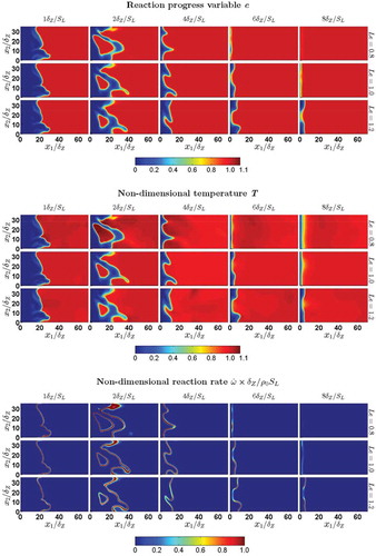
The distributions of reaction progress variable , nondimensional temperature , and the nondimensional reaction rate in the central plane are shown in Figure 1 for turbulent case D for , 1.0, and 1.2. For the unity Lewis number case, c and T are identical when the flame is away from the wall (e.g., ), which is not valid in the and 1.2 cases even when the flame remains away from the wall. The quantities c and T become significantly different from each other in the near-wall region once quenching starts even for . It can be seen from Figure 1 that local super-adiabatic temperatures (i.e., ) are obtained for the nonunity Lewis number flames (i.e., and ). The high values of temperature in the flames are associated with the flame-wrinkles, which are convex towards the reactants, whereas high temperature values in the flames are obtained for flame-wrinkles that are concave towards the reactants. This behavior is consistent with several previous findings (Chakraborty and Cant, 2005, 2009; Rutland and Trouvé, 1993). A combination of strong focusing of reactants and weak defocusing of heat is responsible for high values of temperature and reaction rate magnitude at the wrinkles, which are convexly curved towards the reactants in the cases. Just the opposite mechanism is responsible for high values of temperature in the regions which are concave towards the reactants in the cases. It can be seen from the reaction rate distributions in Figure 1 that the chemical reaction rate drops significantly once the flame reaches in the vicinity of the wall due to a large amount of heat loss through the wall. It has been found that chemical reaction ceases to exist in a region in the , where is the minimum Peclet number, where is the wall Peclet number with being the wall normal distance of isosurafce as defined by Poinsot et al. (1993). The minimum Peclet number for head-on quenching of laminar premixed flames has been found to increase with decreasing (e.g., , 2.83, and 2.75 for , 1.0, and 1.2, respectively). The rate of mass diffusion is greater than the thermal diffusion rate in the case, and thus the reactants from the vicinity of the wall diffuses faster into the approaching flame than the rate of propagation of isotherms towards the wall. As a result, the minimum Peclet number for the laminar flame in the case has been found to be greater than in the unity Lewis number case. The rate of thermal diffusion is greater than the rate of mass diffusion of fresh reactants from the vicinity of the wall in the case, and as a result the isotherms can reach closer to the wall before quenching than in the case. This, in turn, leads to smaller value of in the case than in the case. The values obtained for are consistent with several previous experimental (Huang et al., 1986; Jarosinsky, 1986; Vosen et al., 1984) and computational (Poinsot et al., 1993) findings. The minimum value of wall Peclet number in turbulent flames remains comparable to the corresponding laminar flame value for and 1.2 cases but in the turbulent cases assumes smaller magnitude than the corresponding . The flame quenching is initiated in the turbulent cases when the flame-wrinkles, which are convex towards the wall and associated with super-adiabatic temperatures, approach the wall. The high rate of chemical reaction due to super-adiabatic temperature and relatively weak thermal diffusion rate in turbulent cases enable the aforementioned flame-wrinkles to come closer to the wall than in the corresponding laminar flame before quenching. Although super-adiabatic values of temperature are obtained in the turbulent cases, these high temperature zones are associated with flame-wrinkles, which are concave towards the reactants and as a result quenching of other regions of the flame (which acts to reduce the temperature) starts to occur before these zones interact with the wall. Thus, the minimum Peclet number for the turbulent cases remains comparable to the corresponding laminar values. Interested readers are referred to Lai and Chakraborty (2015) for a more detailed discussion on the influences of on the minimum Peclet number , which is not repeated here for the sake of conciseness.

Figure 1. Distributions of reaction progress variable , nondimensional temperature , and nondimensional reaction rate for turbulent case D with , 1.0, and 1.2 at , , , , on central plane.

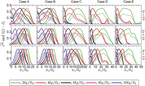
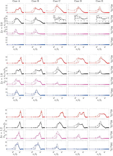
The temporal evolutions of and in the direction normal to the wall are shown in Figure 2. According to Eq. (2), becomes equal to for a presumed bi-modal distribution of with impulse functions at c = 0 and c = 1.0, which is strictly valid for flames (Bray et al., 1985). The difference between and provides a measure of the extent of the deviation of the reaction progress variable pdf from the presumed bi-modal pdf of with impulse functions at c = 0 and c = 1.0. Figure 2 shows that remains smaller than for all cases even when the flames are away from wall (e.g., ) for all Lewis number cases due to small values of Damköhler number (i.e., ). However, later on drops significantly during flame quenching and eventually vanishes in the regions close to the wall, where continues to assume nonzero values (i.e., ). It has been shown by Lai and Chakraborty (2015) that does not resemble a bi-modal distribution in the near-wall region (not shown here for this reason) and thus it is not possible to obtain by an algebraic closure (e.g., Eq. (2)) and under this situation one has to solve a modeled transport equation in order to evaluate .

Figure 2. Variations of (solid line) and (dashed line) with at different time instants for cases A–E (1st–5th columns) and , and .

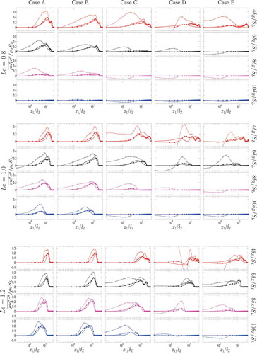
Statistical behavior of the variance transport

The variations of , and with normalized wall normal distance are shown in Figure 3 for all cases considered here. The following observations can be made from the variations of , and with for all cases considered here:

• For all cases the reaction rate term and the molecular dissipation term remain a leading order source and sink terms, respectively, in the variance transport equation when the flame is away from the wall. The magnitudes of both the terms decrease with time as flame starts to quench. The terms and remain the same order of magnitude away from the wall but vanishes in the region given by due to flame quenching, whereas continues to act as a dominant sink term even when disappears. However, eventually vanishes when the flame is completely quenched.

• The mean scalar gradients term acts as a sink for all cases considered here. It can be seen from Figure 3 that the turbulent scalar flux shows counter-gradient transport (i.e., and -) throughout the flame brush for all cases considered here.

• The turbulent transport term shows negative values close to the wall but assumes positive values away from the wall during early stages of flame quenching. However, assumes positive values in the near-wall region and negative values away from the wall as a result of the reversal of flow direction (after quenching the flow is directed towards the wall in contrast to the flow away from the wall before quenching) at later stages of flame quenching.

• One obtains the following scaling estimates of and according to the scaling arguments of Swaminathan and Bray (2005):

(6)

Figure 3. Variations of ,

; ,

; ,

; ,

; ,

with at t = , , , for turbulent cases A–E with , 1.0, and 1.2.

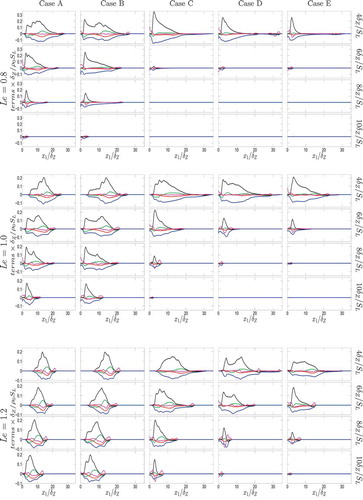
where the gas density is scaled using the unburned gas density , the turbulent velocity fluctuations associated with scalar fluctuations are scaled using the unstrained laminar burning velocity , the mean gradients are scaled using the turbulence integral length scale , and the length scale associated with gradient of fluctuating quantities is scaled using the flame thickness . In Eq. (6), is scaled as . It can be seen from Figure 3 that the magnitudes of the turbulent transport and mean scalar gradient terms and remain smaller than those of and , especially when the flame is away from the wall before flame, which is consistent with the scaling estimates presented in Eq. (6). Furthermore, it can be seen from Figure 3 that the magnitudes of and increase with decreasing , which is consistent with previous findings by Chakraborty and Swaminathan (2011).

The modeling of the terms , and will be discussed next in this article.

Modeling of turbulent transport of scalar variances

According to BML (Bray et al., 1985) the joint pdf between velocity vector and reaction progress variable can be expressed as:

(7)

where , and are the weights associated with the pdf contributions, and are the conditional velocity pdfs in reactants and products, respectively, and originates from the interior of the flame. For high Damköhler number flames the third contribution can be ignored and in the case of unity Lewis number flames one gets: and (Bray et al., 1985). Based on Eq. (7) one gets the following expressions for high Damköhler number (i.e., ) flames (Bray et al., 1985):

(8a)

(8b)

(8c)

where and are the ith components of mean velocity conditional on reactants and products, respectively. The last terms on the right-hand side of Eqs. (8a)–(8c) can be ignored for . Chakraborty and Swaminathan (2011) demonstrated that does not adequately predict obtained from DNS data for low Damköhler number (i.e., ) combustion and proposed an alternative model as:

(9)

where is a model parameter. It is worth to noting that contribution for low Damköhler number (i.e., ) combustion is represented by in Eq. (9). The term accounts for transition of from positive to negative value at the proper location. Moreover becomes unity for high Damköhler number (i.e., ) combustion (because according to Eq. (2)) and thus Eq. (9) becomes identical to Eq. (8c).

For statistically planar flames, remains the only nonzero component of . Figure 4 shows the variations of with normalized wall normal distance as obtained from DNS data along with the predictions of Eq. (9) for all cases considered here. Equation (9) mostly provides satisfactory performance away from the wall but this model underpredicts the magnitude of the negative contribution of in the near-wall region when the flame starts to interact with the wall (see Figure 4). Based on this observation, Eq. (9) has been modified in the following manner:

(10)

Figure 4. Variations of extracted from DNS data (solid line) along with the predictions of Eqs. (9) (dotted line) and (10) (broken line) with at t = , , , for turbulent cases A–E with , 1.0, and 1.2. Please refer to the table in Figure 2 for the color scheme.

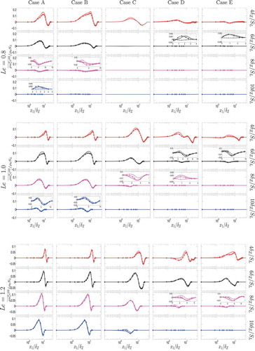
where is the model parameter, which remains active close to the wall where but the magnitude of increases with increasing wall normal distance and asymptotically approach 1.0 away from the wall where . It can be seen from Figure 4 that the model given by Eq. (9) starts to underpredict the magnitude of at an early stage of flame quenching (e.g., t = 8 for and t = 6 for ). Furthermore, Eq. (9) starts to predict the wrong sign of at later stages of flame quenching in cases (e.g., t = 6 for ). The sign of is incorrectly predicted when becomes negative. In order to avoid this discrepancy is introduced in Eq. (10), which assumes a negative value in the near-wall region where remains positive. The term remains active in the near-wall region where and are different from each other as a result of flame quenching. The nonzero value of arises due to different boundary conditions used for the reaction progress variable and nondimensional temperature at the isothermal inert wall (i.e., Dirichlet boundary condition for nondimensional temperature and Neumann boundary condition for reaction progress variable). The ) dependence of ensures that the effects of enthalpy loss due to wall heat transfer are reflected on both the qualitative and quantitative variations of depending on the distance of the flame from the wall. The quantities, and approach each other away from the wall (i.e., ), but and in the near-wall region during flame quenching. A model parameter similar to was previously used in the context of FSD-based closure for flame-wall interaction (Bruneaux et al., 1997). The quantities and approach each other away from the wall (i.e., ), which leads to and thus Eq. (10) reduces to Eq. (9) away from the wall. The wall normal distance at which and approach each other, and the discrepancy between the prediction of Eq. (9) and DNS data depend on (e.g., the discrepancy is greater in extent in the case than in the and 1.2 cases), and thus, is taken to be Lewis number dependent. It can be seen from Figure 4 that the underprediction of by Eq. (9) in the near-wall region can be eliminated by the modification proposed in Eq. (10).

It is worth noting that the success of the model given by Eqs. (8c), (9), and (10) depend on appropriate modeling of turbulent scalar flux . Furthermore, the modeling of plays a pivotal role in the evaluation of . The near-wall modeling of turbulent scalar flux will be addressed next in this article.

Algebraic closure of turbulent scalar flux

Using Eq. (8a) one obtains (Chakraborty and Cant, 2009, 2015; Malkeson and Chakraborty, 2012):

(11)

The slip velocity can be expressed as (Chakraborty and Cant, 2009):

(12)

where is the ith component of the flame normal vector based on the Favre averaged reaction progress variable, is the contribution to the slip velocity arising from turbulence, and is the contribution to the slip velocity arising from heat release. Using Eqs. (11) and (12) one obtains:

(13a)

(13b)

Using (where is a model parameter and is the turbulent kinetic energy) (Chakraborty and Cant, 2009; Veynante et al., 1997) one obtains:

(13c)

The quantity can be scaled as , where is the flame brush thickness. Accordingly, the velocity jump due to heat release over a distance equal to the flame thickness based on reaction progress variable gradient for a corresponding laminar flame (i.e., ) can be estimated as:

(13d)

where is estimated as , in which provides an estimate for the laminar flame thickness based on the reaction progress variable gradient. According to Veynante et al. (1997), can be expressed as , which upon using in Eq. (8b) yields (Chakraborty and Cant, 2009, 2015):

(14)

where and (Chakraborty and Cant, 2015) are the model parameters with and being the the local turbulent Reynolds number and dissipation rate of turbulent kinetic energy , respectively.

For statistically planar flames remains the only nonzero component of . Figure 5 shows the variations of with normalized wall normal distance as obtained from DNS data along with the predictions of Eq. (14) for all cases considered here. It can be seen that is positive throughout the flame brush and gradually reduces zero at the wall. The positive value of is indicative of counter-gradient transport as remains positive in the positive -direction. It can be seen from Figure 5 that Eq. (14) satisfactorily predicts the qualitative behavior of when the flame is away from the wall but this model significantly overpredicts once the flame approaches the wall, and Eq. (14) predicts nonzero values of at the wall. This starts to happen at an earlier time for higher values of because the flame starts to interact with the wall at an earlier time instant due to greater extent of flame wrinkling. In order to eliminate the inadequacies of Eq. (14) in the near-wall region the following modification has been suggested:

(15)

Figure 5. Variations of extracted from DNS data (solid line) along with the predictions of Eqs. (14) (dotted circle line) and (15) (broken triangle line) with at t = , , , for turbulent cases A–E with , 1.0, and 1.2. Please refer to the table in Figure 2 for the color scheme.

where is the model parameter. Figure 5 shows that Eq. (14) overpredicts the magnitude of in the near-wall region. The presence of a wall leads to a decay in velocity fluctuation, which gives rise to a reduction of the magnitude of scalar flux . However, this behavior is not sufficiently captured by Eq. (14) and it overpredicts the magnitude of . For this reason, Eq. (14) is revised to propose a new model (i.e., Eq. 15) where the parameter accounts for the reduction of scalar flux magnitude due to the presence of a wall. The model parameter is responsible for eliminating the overprediction of in the near-wall region. The functional dependence of on ) and ensures that this parameter remains active close to the wall where . The turbulent scalar flux components vanish at the wall (i.e., ) because the velocity component fluctuations vanish at the wall due to no-slip condition. The model parameter contains an error function that depends on , which ensures that both and at . Furthermore, the error function in ensures that it increases from 0 at with increasing and asymptotically approaches 1.0 away from the wall (i.e., ) where Eq. (15) reduces to Eq. (14). The wall normal distance over which and are significantly different from each other depends on Lewis number and this is reflected in dependence of . It can be seen from Figure 5 that Eq. (15) significantly reduces the overprediction of in comparison to Eq. (14) and satisfactorily captures the qualitative behavior of turbulent scalar flux in the near-wall region for all cases considered here.

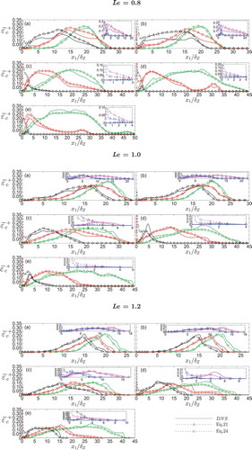
Modeling of reaction rate term

According to Bray et al. (1985), the reaction rate contribution can be expressed as:

(16)

where is given by with being the burning mode pdf. This parameter has been found to be equal to , , and for , 1.0, and 1.2, respectively. Bray (1980) proposed the following closure for the mean reaction rate of reaction progress variable in terms of scalar dissipation rate for flames based on a presumed bi-modal pdf of with impulses at and :

(17)

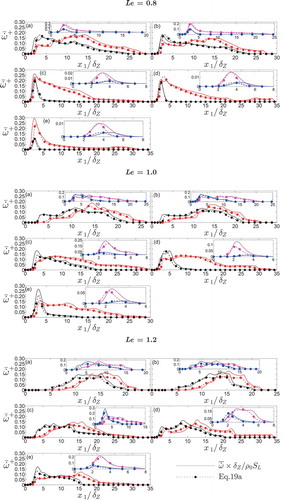
It was shown by Chakraborty and Cant (2011) and Chakraborty and Swaminathan (2011), based on scaling arguments and DNS data, that Eq. (17) also remains valid for as long as the flamelet assumption remains valid. Thus, the reaction rate term can be expressed as:

(18)

Figure 6 shows the variations of with normalized wall normal distance as obtained from DNS data along with the predictions of Eq. (18) for all cases considered here. It can be seen from Figure 6 that Eq. (18) satisfactorily predicts when the flame is away from the wall, but once the quenching starts, Eq. (18) predicts nonzero values at the wall and in the near-wall region, where either vanishes or assumes negligible values. This behavior originates due to nonzero value of in the near-wall region, where vanishes due to flame quenching (Lai and Chakraborty, 2015). Recently, Lai and Chakraborty (2015) extended the expression given by Eq. (18) to predict accurately in the near-wall region in the following manner:

(19a)

Figure 6. Variations of extracted from DNS data (solid line) along with the predictions of Eqs. (18) (dotted circle line) and (20) (broken triangle line) with at t = , , , for turbulent cases A–E with , 1.0, and 1.2. Please refer to the table in Figure 2 for the color scheme.

The parameters , , and in Eq. (19a) are given by:

(19b)

.

In Eq. (19b), and are the Favre averaged values of reaction progress variable and nondimensional temperature at the wall, and is the parameterization for the minimum Peclet number for turbulent flames (see Lai and Chakraborty (2015) for further discussion on this). Equation (19) combines the advantages of both FSD (i.e., , where is the generalized FSD (Boger et al., 1998)) and SDR-based (Eq. (17)) mean reaction rate closures. The FSD-based closure is known to overestimate in the near-wall region during flame quenching (Bruneaux et al., 1997; Lai and Chakraborty, 2015). Moreover, accurately predicts away from the wall for unity Lewis number flames but underpredicts (overpredicts) for the ( cases when the flame is away from the wall (not shown here but interested readers are referred to Lai and Chakraborty (2015) for further information). By contrast, predicts satisfactorily for all cases irrespective of when the flame is away from the wall. In Eq. (19a), the generalized FSD is estimated as and dependence of in ensures that the prediction of Eq. (19a) captures the correct spatial distribution of mean reaction rate at different stages of flame quenching depending on the values of and . The involvement of in the model parameters and ensures that vanishes in the region given by , whereas these model parameters asymptotically approach 1.0 away from the wall (i.e., ). Furthermore, the involvement of implicitly includes reacting boundary layer information into Eq. (19a). For the cases, and are identical to each other for , which leads to and , and thus, Eq. (19a) reduces to Eq. (17). For cases, and are not equal to each other even when the flame is away from wall, and the involvement of Le on the first term on the right-hand side of Eq. (19a) accounts for this effect. The involvement of in the second term on the right-hand side of Eq. (19a) compensates the underprediction (overprediction) of by the FSD-based closure for the turbulent () cases. It can be seen from Figure 7 that Eq. (19a) satisfactorily predicts the mean reaction rate at different stages of flame quenching for all cases considered here.

Figure 7. Variations of with along with the predictions of Eq. (19a) at t = , , , for turbulent cases A–E with , 1.0, and 1.2.

Substituting from Eq. (19a) in Eq. (16) yields the following model for the reaction rate term :

(20)

It can be seen from Figure 6 that Eq. (20) satisfactorily predicts both away and close to the wall for all cases considered here. Equations (19a) and (20) indicate that the satisfactory prediction of and depends on accurate evaluation of SDR . Moreover, the closure of depends on the modeling of . Thus, the modeling of SDR will be discussed next in this article.

Modeling of SDR

Chakraborty and Swaminathan (2011) proposed the following algebraic SDR , which accounts for nonunity Lewis number effects:

(21)

where , , , and are the model parameters; is the local Karlovitz number. In Eq. (21), is a thermochemical parameter, which is defined as (Kolla et al., 2009):

(22)

The parameter is equal to , , and for , 1.0, and 1.2, respectively. It is instructive to present the transport equation of SDR in order to understand the origin of Eq. (21) (Chakraborty et al., 2011; Chakraborty and Swaminathan, 2010; Gao et al., 2015; Mantel and Borghi, 1994; Mura and Borghi, 2003; Swaminathan and Bray, 2005):

(23a)

(23b)

(23c)

(23d)

(23e)

(23f)

(23g)

The first term on the left-hand side of Eq. (23a) is the transient term and the second term on the left-hand side represents the effects of mean advection. The first and second terms on the right-hand side of Eq. (23a) (i.e., and ) denote the molecular diffusion and turbulent transport of , respectively. The term is the density variation term, which arises due to heat release, whereas the turbulence-scalar interaction term arises from the alignment of with local principal strain rates. The terms and denote the contributions of chemical reaction and the molecular dissipation of , respectively. The term arises due to diffusivity gradients.

Equation (21) was derived based on the equilibrium of and . In Eq. 21, the terms , , and originate from the models of , , and , respectively (Chakraborty and Swaminathan, 2010; Chakraborty and Swaminathan, 2011). It was shown by Lai and Chakraborty (2015) that this equilibrium between and has been obtained away from the wall (i.e., ) but such an equilibrium is not maintained in the near-wall region (i.e., ). The Lewis number dependences in and account for strengthening of the density variation term and the contribution of turbulence-scalar interaction arising from the strain rate due to flame normal acceleration as a result of augmented chemical heat release for small values of (Chakraborty and Swaminathan, 2010, 2011).

Figure 8 shows the variations of with normalized wall normal distance as obtained from DNS data along with the predictions of Eq. (21) for all cases considered here. It can be seen from Figure 8 that Eq. (21) significantly overpredicts in the near-wall region where the equilibrium between and is not maintained (Lai and Chakraborty, 2015). Thus, Eq. (21) yields an erroneous value of dissipation rate term ( and SDR in the near-wall region (). Lai and Chakraborty (2015) modified Eq. (21) in the following manner in order to account for the near-wall behavior:

(24)

Figure 8. Variations of obtained from DNS data and the predictions of Eqs. (21) and (24) with at t = , , , for turbulent cases A–E with , 1.0, and 1.2. Please refer to the table in Figure 2 for the color scheme.

where the model parameters and only remain active close to the wall to account for the flame-wall interaction and they asymptotyically approach 1.0 away from the wall. The involvement of includes reacting boundary layer information into the model given by Eq. (24). Furthermore, ) dependence of Eq. (24) accounts for the effects of nonadiabaticity due to wall heat transfer, which influences both the qualitative and quantitative variations of depending on the distance of the flame from the wall. Figure 8 shows that Eq. (24) predicts accurately for both near to and away from the wall.

Conclusions

The reaction progress variable variance transport and its modeling in the context of RANS have been analyzed for head-on quenching of turbulent premixed flame due to an inert isothermal wall using 3D simple chemistry DNS data for global Lewis numbers ranging from 0.8 to 1.2. The statistical behaviors of the unclosed terms in the transport equation of have been analyzed in detail and their relative magnitudes have been explained based on scaling arguments. It has been found that the reaction rate contribution and the molecular dissipation term are the leading order source and sink terms, respectively, in the transport equation. However, the reaction rate contribution vanishes in the near-wall region due to flame quenching, whereas continues to act as a dominant sink. The mean scalar gradient term acts as the sink term for all cases considered here, since the turbulent scalar flux shows counter-gradient transport in these cases. The turbulent flux of scalar variance assumes positive values in the near-wall region but becomes negative away from the wall at early stages of flame quenching but an opposite behavior is observed at the final stage of quenching. The performances of previously proposed models for turbulent fluxes and , reaction rate contribution and scalar dissipation rate have been assessed with respect to the corresponding quantities extracted from DNS data. It has been found that the aforementioned models do not adequately predict the near-wall behavior of the unclosed terms of the variance transport equation. The existing models for the unclosed terms of the variance transport equation have been modified to account for the near-wall behavior in such a manner that the modified models asymptotically approach the existing model expressions away from the wall. The functional forms of the modeling parameters have been proposed in such a manner that they follow the asymptotic behavior in terms of normalized wall normal distance . It is, however, likely that they need to be validated further based on both experimental and DNS data for high values of . Furthermore, the proposed models need to be implemented in actual RANS simulations to assess their predictive capabilities. Some of the aforementioned issues will form the basis of future analyses.

Acknowledgment

The authors are grateful to N8/ARCHER (EP/K025163/1) for the computational support.

Funding

The authors gratefully acknowledge the School of Mechanical and Systems Engineering of Newcastle University for the financial support.

References

• Alshaalan, T.M., and Rutland, C.J. 1998. Turbulence, scalar transport, and reaction rates in flame-wall interaction. Proc. Combust. Inst., 27, 793.
   Google Scholar
• Alshaalan, T.M., and Rutland, C.J. 2002. Wall heat flux in turbulent premixed reacting flow. Combust. Sci. Technol., 174, 135.
   Web of Science ®Google Scholar
• Bachelor, G.K., and Townsend, A.A. 1948. Decay of turbulence in final period. Proc. R. Soc. London, Ser. A, 194, 527.
   Web of Science ®Google Scholar
• Boger, M., Veynante, D., Boughanem, H., and Trouvé, A. 1998. Direct numerical simulation analysis of flame surface density concept for large eddy simulation of turbulent premixed combustion. Proc. Combust. Inst., 27, 917.
   Google Scholar
• Bray, K.N.C. 1980. Turbulent flows with premixed reactants. In P.A. Libby and F.A. Williams (Eds.), Turbulent Reacting Flows, Springer Verlag, Berlin Heidelburg, New York, pp. 115–183.
   Google Scholar
• Bray, K.N.C., Champion, M., and Libby, P.A. 2006. Finite rate chemistry and presumed PDF models for premixed turbulent combustion. Combust. Flame, 145, 665–673.
   Web of Science ®Google Scholar
• Bray, K.N.C., Libby, P.A., and Moss, J.B. 1985. Unified modelling approach for premixed turbulent combustion—Part I: General formulation. Combust. Flame, 61, 87.
   Web of Science ®Google Scholar
• Bruneaux, G., Akselvoll, K., Poinsot, T., and Ferziger, J.H. 1996. Flame-wall interaction simulations in a turbulent channel flow. Combust. Flame, 107, 27.
   Web of Science ®Google Scholar
• Bruneaux, G., Poinsot, T., and Ferziger, J.H. 1997. Premixed flame-wall interaction in a turbulent channel flow: Budget for the flame surface density evolution equation and modelling. J. Fluid. Mech., 349, 191.
   Web of Science ®Google Scholar
• Chakraborty, N., and Cant, R.S. 2005. Influence of Lewis number on curvature effects in turbulent premixed flame propagation in the thin reaction zones regime. Phys. Fluids, 17, 105105.
   Web of Science ®Google Scholar
• Chakraborty, N., and Cant, R.S. 2009. Effects of Lewis number on turbulent scalar transport and its modelling in turbulent premixed flames. Combust. Flame, 156, 1427.
   Web of Science ®Google Scholar
• Chakraborty, N., and Cant, R.S. 2015. Effects of turbulent Reynolds number on turbulent scalar flux modeling in premixed flames using Reynolds-Averaged Navier-Stokes simulations. Numer. Heat Transfer, 67, 1187.
   Web of Science ®Google Scholar
• Chakraborty, N., and Cant, R.S. 2011. Effects of Lewis number on flame surface density transport in turbulent premixed combustion. Combust. Flame, 158, 1768.
   Web of Science ®Google Scholar
• Chakraborty, N., Champion, M., Mura, A., and Swaminathan, N. 2011. Scalar dissipation rate approach to reaction rate closure. In: N. Swaminathan and K.N.C. Bray (Eds.), Turbulent Premixed Flame, 1st ed., Cambridge University Press, Cambridge, UK, pp. 76–102.
   Google Scholar
• Chakraborty, N., and Swaminathan, N. 2010. Effects of Lewis number on scalar dissipation transport and its modelling implications for turbulent premixed combustion. Combust. Sci. Technol., 182, 1201.
   Web of Science ®Google Scholar
• Chakraborty, N., and Swaminathan, N. 2011. Effects of Lewis number on scalar variance transport in premixed flames. Flow Turbul. Combust., 87, 261.
   Web of Science ®Google Scholar
• Chen, J.H., Choudhary, A., de Supinski, M., de Vries, B., Hawkes, E.R., Klasky, S., Liao, W.K., Ma, K.L., Mellor-Crummey, J., Podhorski, N., Sankaran, R., Shende, S., and Yoo, C.S. 2009. Terascale direct numerical simulations of turbulent combustion using S3D. Comput. Sci. Discovery, 2, 015001.
   Google Scholar
• Clavin, P., and Williams, F.A. 1982. Effects of molecular diffusion and thermal expansion on the structure and dynamics of turbulent premixed flames in turbulent flows of large scale and small intensity. J. Fluid Mech., 128, 251.
   Web of Science ®Google Scholar
• Dabireau, F., Cuenot, B., Vermorel, O., and Poinsot, T. 2003. Interaction of flames of H2–O2 with inert walls. Combust. Flame, 135, 123.
   Web of Science ®Google Scholar
• Dinkelacker, F., Manickam, B., and Mupppala, S. 2011. Modelling and simulation of lean premixed turbulent methane/hydrogen/air flames with an effective Lewis number approach. Combust. Flame, 158, 1747.
   Web of Science ®Google Scholar
• Domingo, P., Vervisch, L., Payet, S., and Hauguel, R. 2005. DNS of a premixed turbulent V-flame and LES of a ducted flame using a FSD-PDF subgrid scale closure with FPI tabulated chemistry. Combust. Flame, 143, 566.
   Web of Science ®Google Scholar
• Gao, Y., Chakraborty, N., Dunstan, T.D., and Swaminathan, N. 2015. Assessment of Reynolds Averaged Navier Stokes modelling of scalar dissipation rate transport in turbulent oblique premixed flames. Combust. Sci. Technol., 187(10), 1584.
   Web of Science ®Google Scholar
• Gruber, A., Chen, J.H., Valiev, D., and Law, C.K. 2012. Direct numerical simulation of premixed flame boundary layer flashback in turbulent channel flow. J. Fluid Mech., 709, 516.
   Web of Science ®Google Scholar
• Gruber, A., Sankaran, R., Hawkes, E.R., and Chen, J.H. 2010. Turbulent flame-wall interaction: A direct numerical simulation study. J. Fluid. Mech., 658, 5.
   Web of Science ®Google Scholar
• Han, I., and Huh, K.H. 2008. Roles of displacement speed on evolution of flame surface density for different turbulent intensities and Lewis numbers for turbulent premixed combustion. Combust. Flame, 152, 194.
   Web of Science ®Google Scholar
• Haworth, D.C., and Poinsot, T.J. 1992. Numerical simulations of Lewis number effects in turbulent premixed flames. J. Fluid Mech., 244, 405.
   Web of Science ®Google Scholar
• Huang, W.M., Vosen, S.R., and Greif, R. 1986. Heat transfer during laminar flame quenching. Proc. Combust. Inst., 21, 1853.
   Google Scholar
• Im, H.G., and Chen, J.H. 2002. Preferential diffusion effects on the burning rate of interacting turbulent premixed hydrogen-air flames. Combust. Flame, 131, 246.
   Web of Science ®Google Scholar
• Jarosinsky, J. 1986. A survey of recent studies on flame extinction. Combust. Sci. Technol., 12, 81.
   Web of Science ®Google Scholar
• Jenkins, K.W., and Cant, R.S. 1999. Direct numerical simulation of turbulent flame kernel. In Recent Advances in DNS and LES: Proceedings of the Second AFOSR Conference, D. Knight and L. Sakell (Eds.), Rutgers—The State University of New Jersey, New Brunswick, NJ, June 7–9; Kluwer Academic Publishers, New York, pp. 191–202.
   Google Scholar
• Klimenko, A.Y., and Bilger, R.W. 1999. Conditional moment closure for turbulent condition. Prog. Energy Combust. Sci., 25, 595.
   Web of Science ®Google Scholar
• Kolla, H., Rogerson, J.W., Chakraborty, N., and Swaminathan, N. 2009. Scalar dissipation rate modeling and its validation. Combust. Sci. Technol., 181, 518.
   Web of Science ®Google Scholar
• Lai, J., and Chakraborty, N. 2015. Effects of Lewis number on head on quenching of turbulent premixed flame: A direct numerical simulation analysis. Flow Turbul. Combust, 96, 279–308.
   Web of Science ®Google Scholar
• Law, C.K., and Kwon, O.C. 2004. Effects of hydrocarbon substitution on atmospheric hydrogen–air flame propagation. Int. J. Hydrogen Energy, 29, 867.
   Web of Science ®Google Scholar
• Libby, P.A., Linan, A., and Williams, F.A. 1983. Strained premixed laminar flames with non-unity Lewis number. Combust. Sci. Technol., 34, 257.
   Web of Science ®Google Scholar
• Linstedt, R.P., and Vaos, E.M. 1999. Modelling of premixed turbulent flames with second moment methods. Combust. Flame, 116, 46.
   Web of Science ®Google Scholar
• Malkeson, S.P., and Chakraborty, N. 2010. Modelling of fuel mass fraction variance transport in turbulent stratified flames: A direct numerical simulation study. Numer. Heat Transfer A, 58, 187.
   Web of Science ®Google Scholar
• Malkeson, S.P., and Chakraborty, N. 2012. A-priori DNS modelling of the turbulent scalar fluxes for low Damköhler number stratified flames. Combust. Sci. Technol., 184, 1680.
   Web of Science ®Google Scholar
• Mantel, T., and Bilger, R.W. 1995. Conditional statistics in a turbulent premixed flame derived from direct numerical simulation. Combust. Sci. Technol., 96(3), 393.
   Google Scholar
• Mantel, T., and Borghi, R. 1994. A new model of premixed wrinkled flame propagation based on a scalar dissipation equation. Combust. Flame, 96, 443.
   Web of Science ®Google Scholar
• Mizomoto, M., Asaka, S., Ikai, S., and Law, C.K. 1984. Effects of preferential diffusion on the burning intensity of curved flames. Proc. Combust. Inst., 20, 1933.
   Google Scholar
• Moler, S.I., Lundgren, E., and Fureby, C. 1996. Large eddy simulation of turbulent combustion. Proc. Combust. Inst., 26, 241–248.
   Google Scholar
• Mura, A., and Borghi, R. 2003. Towards an extended scalar dissipation equation for turbulent premixed combustion. Combust. Flame, 133, 193.
   Web of Science ®Google Scholar
• Mura, A., Robin, V., and Champion, M. 2007. Modelling of scalar dissipation in partially premixed flames. Combust. Flame, 149, 217.
   Web of Science ®Google Scholar
• Poinsot, T.J., Haworth, D.C., and Bruneaux, G. 1993. Direct simulation and modelling of flame-wall interaction for premixed turbulent combustion. Combust. Flame, 95, 118.
   Web of Science ®Google Scholar
• Poinsot, T.J., and Lele, S. 1992. Boundary conditions for direct simulations of compressible viscous flows. J. Comput. Phys., 10, 104.
   Web of Science ®Google Scholar
• Ribert, G., Champion, M., Gicquel, O., Darabiha, N., and Veynante, D. 2005. Modeling of nonadiabatic turbulent premixed reactive flows including tabulated chemistry. Combust. Flame, 141, 271–280.
   Web of Science ®Google Scholar
• Robin, V., Mura, A., Champion, M., and Plion, P. 2006. A multi-Dirac presumed PDF model for turbulent reacting flows with variable equivalence ratio. Combust. Sci. Technol., 178, 1843.
   Web of Science ®Google Scholar
• Rogallo, R.S. 1981. Numerical experiments in homogeneous turbulence. NASA Technical Memorandum 81315. NASA Ames Research Center, Moffett Field, CA.
   Google Scholar
• Rutland, C., and Trouvé, A. 1993. Direct simulations of premixed turbulent flames with nonunity Lewis numbers. Combust. Flame, 94, 41.
   Web of Science ®Google Scholar
• Savre, J., Bertier, N., and Gaffie, D. 2008. A flamelet tabulated chemistry approach for premixed combustion using industrial CFD codes. Presented at the 2nd Colloquium INCA, CORIA, Rouen, France, October 23–24.
   Google Scholar
• Sivashinsky, G.I. 1977. Diffusional-thermal theory of cellular flames. Combust. Sci. Technol., 16, 137.
   Web of Science ®Google Scholar
• Swaminathan, N., and Bilger, R.W. 2001. Analyses of conditional moment closure for turbulent premixed flames. Combust. Theor. Model., 5, 1.
   Web of Science ®Google Scholar
• Swaminathan, N., and Bray, K.N.C. 2005. Effect of dilatation on scalar dissipation in turbulent premixed flames. Combust. Flame, 143, 549.
   Web of Science ®Google Scholar
• Swaminathan, N., and Bray, K.N.C. 2011. Fundamentals and challenges. In N. Swaminathan and K.N.C. Bray (Eds.), Turbulent Premixed Flame, 1st ed., Cambridge University Press, Cambridge, UK, pp. 1–40.
   Google Scholar
• Trouvé, A., and Poinsot, T. 1994. The evolution equation for flame surface density in turbulent premixed combustion. J. Fluid Mech., 278, 1.
   Web of Science ®Google Scholar
• Veynante, D., Trouvé, A., Bray, K.N.C., and Mantel, T. 1997. Gradient and countergradient turbulent scalar transport in turbulent premixed flames. J. Fluid Mech., 332, 263.
   Web of Science ®Google Scholar
• Vosen, S.R., Greif, R., and Westbrook, C. 1984. Unsteady heat transfer in laminar flame quenching. Proc. Combust. Inst., 20, 76.
   Google Scholar
• Wray, A.A. 1990. Minimal storage time advancement schemes for spectral methods. NASA Ames Research Center, California.
   Google Scholar

Additional information

Funding

The authors gratefully acknowledge the School of Mechanical and Systems Engineering of Newcastle University for the financial support.