Statistical Analysis of the Reaction Progress Variable and Mixture Fraction Gradients in Flames Propagating into Droplet Mist: A Direct Numerical Simulation Analysis

ABSTRACT

The statistics of reaction progress variable, , and mixture fraction, , and their gradients (i.e., and ) in flames propagating in droplet mist, where the fuel was supplied in the form of monodisperse droplets, have been analyzed for different values of turbulent velocity fluctuations (), droplet equivalence ratios (, and droplet diameters ( based on three-dimensional direct numerical simulations (DNS) in a canonical configuration under decaying turbulence. The combustion process in the gaseous phase has been found to take place predominantly in fuel-lean mode, even for . The probability of finding fuel-lean mixture increases with increasing initial droplet diameter due to slower evaporation of larger droplets. It has been shown that the joint probability density function (i.e., joint PDF) of and (i.e., ), cannot be approximated in terms of discrete delta functions throughout the flame brush for the cases considered here. Furthermore, the magnitude of cannot be adequately approximated by the product of marginal PDFs of , and variable, (i.e., ). The statistical properties of the Favre probability density functions (Favre-PDFs) of the mixture fraction, , and oxidizer-based reaction progress variable, , have been analyzed at several locations across the flame brush and a -function distribution has been found to capture the Favre-PDFs of and obtained from the DNS data. Furthermore, a log-normal distribution has been shown to capture the qualitative behaviors of the PDFs of the gradient of the mixture fraction and the gradient of the reaction progress variable, and , respectively, but discrepancies between the log-normal distribution and the DNS data were observed at the tails of PDFs. In addition, the interrelation between and was examined in terms of the PDFs of the cosine of the angle between them (i.e., and it was observed that most droplet cases exhibited much greater likelihood of positive values of than negative values. Finally, the joint PDF of and , , has been compared with that of P( (i.e., assuming statistical independence of and ) and a good level of agreement has been obtained. The bivariate log-normal distribution has been considered both assuming correlation between and and assuming no correlation for the purpose of modeling , and the variant with no correlation has been found to be more successful in capturing qualitative behavior of although quantitative discrepancies have been observed due to inaccuracies involved in parameterizing P( and P(by log-normal distributions.

KEYWORDS:

• Direct numerical simulation
• Droplet combustion
• Mixture fraction
• Probability density function
• Reaction progress variable

Introduction

Flame propagation into turbulent droplet-laden mixtures is of pivotal relevance to several engineering applications ranging from Internal Combustion (IC) engines to aero-gas turbines to the prediction and control of hazards (Aggarwal, 1998; Heywood, 1998; Lefebvre, 1998). A number of experimental (Aggarwal and Sirignano, 1985; Ballal and Lefebvre, 1981; Burgoyne and Cohen, 1954; Faeth, 1987; Hayashi et al., 1976; Lawes and Saat, 2011; Nomura et al., 2000; Szekely and Faeth, 1983), analytical (Greenberg et al., 1998; Greenberg et al., 2009; Silverman et al., 1993), and computational (Fujita et al., 2013; Wacks et al., 2015; Watanbe et al., 2007, 2008) analyses concentrated on flame propagation in turbulent droplet-laden mixtures and indicated a complex physical interaction of evaporative heat and mass transfer, fluid dynamics, and combustion thermo-chemistry is responsible for flame droplet interaction. The experimental evidence suggested that there could be significant differences between the overall equivalence ratio (considering fuel in both liquid and gaseous phases) and gaseous equivalence ratio due to incomplete evaporation. Furthermore, droplet inertia along with the difference between overall and gaseous equivalence ratios could give rise to augmentation/reduction of burning rate in quiescent and low turbulence conditions, but that these effects disappear for sufficiently high turbulence intensity (Aggarwal and Sirignano, 1985; Lawes and Saat, 2011; Nomura et al., 2000). Recently, direct numerical simulations (DNS) have made significant contributions to both the physical understanding and modeling of the combustion of turbulent droplet-laden mixtures (Luo et al., 2011; Miller and Bellan, 1999; Neophytou et al., 2010, 2011, 2012; Reveillon and Demoulin, 2007; Reveillon and Vervisch, 2000; Sreedhara and Huh, 2007; Wandel, 2013, 2014; Wandel et al., 2009; Wang and Rutland, 2005; Xia and Luo, 2010). Neophytou and Mastorakos (2009) recently analyzed the effects of volatility, droplet diameter, and droplet equivalence ratio on burning velocity in one-dimensional (1D) laminar flames where fuel is supplied in the form of monodisperse droplets. Wacks et al. (2015) recently extended the analysis of Neophytou and Mastorakos (2009) for turbulent flames by carrying out 3D compressible DNS of freely propagating turbulent flame propagation into droplet-laden mixtures.

The statistical behaviors of the gradients of mixture fraction and reaction progress variable have been analyzed in several previous analyses on partially premixed and stratified flames (Bray et al., 2005; Malkeson et al., 2013; Ruan et al., 2012), where mixture fraction and reaction progress variable are taken to be representative passive and active scalars. Although mixture fraction is not strictly a passive scalar in the case of spray combustion, the mixture inhomogeneity in the gaseous phase in spray flames is often characterized in terms of mixture fraction (Ge and Gutheil, 2006; Sadiki et al. 2012). Furthermore, the progress of chemical reaction in inhomogeneous mixtures in droplet combustion can be characterized by reaction progress variable , which can be defined in terms of a suitable species mass fraction so that it assumes a value equal to zero in the unburned gas and monotonically increases to assume a value equal to unity in the fully burned gas. The interdependence of mixture fraction and reaction progress variable plays a key role in the modeling of spray combustion using flamelet generated manifold (FGM) (Ma et al., 2014; Sadiki et al., 2012). Furthermore, the characterization of probability density functions (PDFs) of mixture fraction and reaction progress variable and their respective gradients (i.e., and ) in terms of presumed functions play pivotal roles in flamelet and conditional moment closures (CMC; Borghesi et al., 2011; Ge and Gutheil, 2006; Sadiki et al., 2012; Tyliszczak et al., 2014). Furthermore, the statistics of and play key roles in determining the statistical behaviors of scalar dissipation rates and and cross-scalar dissipation rate , which are necessary for the purpose of modeling turbulent combustion in partially premixed mixtures (Bray et al., 2005; Malkeson et al., 2013; Ribert et al., 2005; Robin et al., 2006; Ruan et al., 2012). These modeling issues will also be valid for droplet combustion because the evaporation of droplets will lead to partially premixed combustion in gaseous phase. Although different presumed PDF approaches have been used in the past in the context of spray combustion (Ge and Gutheil, 2006; Ma et al., 2014; Sadiki et al., 2012; Tyliszczak et al., 2014), the statistics of the interdependence of and reaction progress variable and their gradients (i.e., and ) have received limited attention (Luo et al., 2011; Wandel, 2013, 2014; Xia and Luo, 2010) in existing literature. This deficit has been addressed here by analyzing the statistical behavior of and , and their respective gradients (i.e., and ) based on 3D DNS data of freely propagating statistically planar turbulent flames propagating into droplet mist for different values of root-mean-square velocity fluctuation droplet diameter , and droplet equivalence ratio , where in which is the mass of fuel in droplet form, is the mass of oxidizer, and is the ratio of the mass of fuel to the mass of oxidizer in the stoichiometric mixture. In this respect, the main objectives of the present analysis are:

1. To analyze the distributions of and and their joint PDF within the flame front for turbulent spray flames for different values of , and .

2. To analyze the influences of , and on the statistical behaviors of and and their interdependence.

3. To provide physical explanations for the aforementioned statistical behaviors and indicate modeling implications.

The remainder of the article takes the following form. The necessary mathematical background and information related to the numerical implementation are provided in the next two sections. Following this, the results are presented and subsequently discussed, and finally, the main findings are summarized and conclusions are drawn.

Mathematical background

A single-step irreversible Arrhenius-type chemical mechanism has been used for the purpose of carrying out the present extensive parametric analysis without an exorbitant computational cost:

(1)

where is the oxidizer-fuel ratio by mass (i.e., the mass of oxygen consumed per unit mass of fuel). The fuel reaction rate is expressed as:

(2)

where and are the fuel and oxygen mass fractions, respectively, and is the gas density. In Eq. (2), , the nondimensional temperature; , the Zeldovich number; , a heat release parameter; and , the normalized pre-exponential factor, are given by the following expressions:

(3)

where is the instantaneous dimensional temperature, is the unburned gas temperature, is the adiabatic flame temperature for the stoichiometric mixture, is the activation energy, is the universal gas constant, is the pre-exponential factor, and is a heat release parameter. Here, the modified single step chemical mechanism proposed by Tarrazo et al. (2006) has been considered and in this framework the activation energy, , and the heat of combustion are taken to be functions of the gaseous equivalence ratio, , which results in more accurate predictions of the equivalence ratio dependence of the unstrained laminar burning velocity in hydrocarbon-air flames, especially for fuel-rich mixtures. According to Tarrazo et al. (2006), the Zel’dovich number, , is expressed as where:

(4)

According to Tarrazo et al. (2006), the heat release per unit mass of fuel is given by for and for , where , and and are the fuel mass fraction in the unburned gas and fully burned gas, respectively, for a premixed flame of equivalence ratio . For the present investigation, the Lewis numbers of all species are taken to be equal to unity and all species in the gaseous phase are considered to be perfect gases. Standard values have been taken for the ratio of specific heats (, where and are the specific heats at constant pressure and volume for the gaseous mixture, respectively) and Prandtl number (, where and are the dynamic viscosity and thermal conductivity, respectively).

The droplet transport equations used in several previous analyses (Luo et al., 2011; Neophytou et al., 2010, 2011, 2012; Reveillon and Demoulin, 2007; Reveillon and Vervisch, 2000; Sreedhara and Huh, 2007; Wandel, 2013, 2014; Wandel et al., 2009; Wang and Rutland, 2005; Xia and Luo, 2010) have been adopted for this analysis. The position, , velocity, , diameter, , and temperature, , for individual droplets are tracked in Lagrangian manner, and the relevant transport equations for these quantities are given by:

(5)

(6)

(7)

(8)

where is the latent heat of vaporization, and , , and are relaxation timescales associated with droplet velocity, diameter, and temperature, respectively, which are given by:

(9)

where is the droplet density, is the specific heat for the fuel in liquid phase, is the correction for drag coefficient and is expressed as (Clift et al., 1978):

(10)

In Eq. (10), is the droplet Reynolds number, is the Schmidt number, is the Spalding mass transfer number, is the corrected Sherwood number, and is the corrected Nusselt number, which are expressed as (Clift et al., 1978; Luo et al., 2011; Neophytou et al., 2010, 2011, 2012; Reveillon and Vervisch, 2000; Wandel, 2013, 2014; Wandel et al., 2009; Xia and Luo, 2010):

(11)

(12)

(13)

where is the value of fuel mass fraction on the droplet surface. It is worth noting that the unity Lewis number assumption has been implicitly invoked in Eqs. (11)–(13). Furthermore, the Clausius–Clapeyron relation for the partial pressure of the fuel vapor at the droplet surface, , is utilized to calculate the Spalding number :

(14)

where is the boiling point of the fuel at reference pressure , the droplet surface temperature is taken to be , and and are the molecular weights of oxidizer and fuel, respectively.

The conservation equations in the gaseous phase can be generically written as (Neophytou et al., 2010, 2011, 2012; Reveillon and Vervisch, 2000; Wandel, 2013, 2014; Wandel et al., 2009):

(15a)

where for the transport equations of mass, momentum, energy, and mass fractions, respectively; for and and for and , respectively, with and being the velocity in the jth direction and the specific stagnation internal energy respectively. The quantity is an appropriate Schmidt number corresponding to . The term in Eq. (15a) arises due to chemical reaction rate, and and are the appropriate source terms in the gaseous phase and are due to droplet evaporation, respectively. The droplet source term is tri-linearly interpolated from the droplet’s sub-grid position, , to the eight surrounding nodes. The droplet source term for any variable may be expressed as (Neophytou et al., 2010, 2011, 2012; Wandel, 2013, 2014; Wandel et al., 2009):

(15b)

where is the cell volume, is the droplet mass and the summation is carried out over all droplets in the vicinity of each node. As indicated in Eq. (15a), the variable is identified as , however, since within the droplets , the source term for both the continuity equation and the fuel mass fraction equation are identical.

Evaporation of droplets leads to mixture inhomogeneities, which is often quantified in terms of the mixture fraction, which is defined as:

(16)

where is the fuel mass fraction in the pure fuel stream and is the oxidizer mass fraction in air. The hydrocarbon fuel used in this DNS analysis is n-heptane, , for which and the stoichiometric fuel mass fraction and mixture fraction values are given by . Furthermore, it is possible to define a reaction progress variable,, based on a species mass fraction and the mixture fraction such that rises monotonically from zero in the unburned reactants to one in the fully burned products. Here, the progress variable, , has been defined in terms of oxidizer mass fraction in the following manner following several previous analyses (Neophytou et al., 2010, 2011, 2012; Wandel, 2014; Wandel et al., 2009):

(17)

From Eq. (17) it is possible to derive a transport equation of based on the transport equations for the oxidizer mass fraction and the mixture fraction (Bray et al., 2005; Wacks et al., 2015):

(18)

where is the mass diffusivity and the first term on the right-hand side of Eq. (18) arises due to molecular diffusion, the second term represents reaction rate, the third is the source/sink term arising due to droplet evaporation, and the last is the cross-scalar dissipation term arising due to reactant inhomogeneity (Bray et al., 2005; Malkeson and Chakraborty, 2010; Wacks et al., 2015). The cross-scalar dissipation term in Eq. (18) arises due to mixture inhomogeneity (Bray et al., 2005; Malkeson and Chakraborty, 2010; Wacks et al., 2015), which, in this case, is induced by droplet evaporation. According to the definition of (see Eq. (17)), the definitions of , , and depend on the local value of . The expressions for and are given by the following expressions (Wacks et al., 2015):

(19)

(20)

where is the droplet source/sink term in the mixture fraction transport equation and and are the droplet source/sink terms in the fuel and oxidizer transport equations, respectively, and is the source term in the mass conservation equation due to evaporation.

The reaction rate of the reaction progress variable may be expressed as (Bray et al., 2005; Malkeson et al., 2013; Ruan et al., 2012):

(21)

where is the (cross-)scalar dissipation rate, for scalars and (here or ). It is evident from Eq. (21) that the evaluation of (cross-)scalar dissipation rates is essential to accurately model . In the context of Reynolds averaged Navier–Stokes (RANS) simulations, the Favre-averaged (cross-)scalar dissipation rates, (where the Favre mean and Favre fluctuation of a scalar are given by and , respectively, with the overbar indicating a suitable Reynolds averaging operation) must be modeled. For RANS, the components of scalar dissipation and cross-scalar dissipation rates arising from the mean gradients are negligible in comparison to the contributions from gradients of fluctuations (i.e., , , and ), which gives rise to the following expressions:

(22)

The scalar dissipation rates , and can alternatively be expressed as:

(23a)

(23b)

(23c)

where is the joint PDF of quantities and . Equations (23a)–(23c) indicate that the statistical behaviors of , , , and are of fundamental interest for the purpose of modeling of , , and (Malkeson et al., 2013; Ruan et al., 2012). The statistical behaviors of , , , and will be discussed in the Results and discussion section of this article.

Numerical implementation

A widely-used 3D compressible DNS code SENGA (Jenkins and Cant, 1999; Neophytou et al., 2010, 2011, 2012; Wandel, 2013, 2014; Wandel et al., 2009; Wacks et al., 2015), which solves the standard transport equations of mass, momentum, energy, and species in nondimensional form has been employed for this analysis. In this framework, the spatial discretization for the internal grid points has been carried out using a 10th-order central difference scheme, where the order of differentiation drops gradually to a one-sided 2nd-order scheme at the nonperiodic boundaries (Jenkins and Cant, 1999). A low-storage third-order explicit Runge–Kutta scheme has been used for time advancement (Wray, 1990). A rectangular computational domain of size has been considered for the current investigation, where is the unburned gas diffusivity. For the present thermo-chemistry the Zel’dovich flame thickness is equal to about where is the unstrained thermal laminar flame thickness of the stoichiometric laminar flame, and the subscript refers to the values in an unstrained laminar premixed flame for the stoichiometric mixture. The simulation domain for the present analysis is discretized using a Cartesian grid of size , which resolves both the flame thickness, , and the Kolmogorov length-scale, . The boundaries in the mean direction of flame propagation (i.e., x-direction) are taken to be partially nonreflecting, whereas the transverse (i.e., y- and z-) directions are assumed to be periodic. The Navier–Stokes characteristic boundary conditions (NSCBC) (Poinsot and Lele, 1992) technique has been used for specifying the nonperiodic boundary conditions. The droplets are distributed uniformly in space throughout the y- and z-directions and in the region ahead of the flame. The initial conditions for the reacting flow field have been generated based on the steady laminar solution obtained for the desired initial values of droplet diameter, , and droplet equivalence ratio, . This initial condition has been generated using COSILAB (Neophytou and Mastorakos, 2009), where the 1D governing equations for the gas and liquid phases are solved in a coupled manner for spray flames where fuel is supplied in the form of monodisperse droplets on the unburned gas side of the flame. The turbulent velocity fluctuations have been initialized using a standard pseudo-spectral method (Rogallo, 1981), and this field is superimposed on the steady laminar spray flame solution generated using COSILAB. For the present analysis the unburned gas temperature is , which gives rise to a heat release parameter . For all simulations, the fuel is supplied purely in the form of monodisperse droplets with nondimensional diameters for different values of droplet equivalence ratio: at a distance from the point in the laminar flame at which , which corresponds to a nondimensional temperature . The droplet number density at varies between in the region . In all cases the liquid volume fraction remains much smaller than . In all cases droplets are supplied at the left-hand-side boundary to maintain a constant ahead of the flame. The droplets evaporate as they approach the flame front and the droplet diameter decreases by at least 25% by the time it reaches the most reactive region of the flame, such that the volume of even the largest droplets is now less than half that of the cell volume, which validates the sub-grid point source treatment of droplets adopted for flame-droplet interactions analyzed here since this study is concerned primarily with regions where reaction rate is non-negligible. This droplet to cell size for the present analysis is consistent with several previous analyses (Neophytou et al., 2010, 2011, 2012; Reveillon and Vervisch, 2000; Sreedhara and Huh, 2007; Wandel, 2013, 2014; Wandel et al., 2009; Wang and Rutland, 2005).

The simulations are carried out for normalized root-mean-square (rms) turbulent velocities and with a nondimensional longitudinal integral length-scale . The ratio of droplet diameter to the Kolmogorov scale is for , respectively, for initial , and these ratios are larger in magnitude for the cases with . The ratio of remains comparable to several previous analyses (Neophytou et al., 2010, 2011, 2012; Reveillon and Vervisch, 2000; Sreedhara and Huh, 2007; Wandel, 2013, 2014; Wandel et al., 2009; Wang and Rutland, 2005). The mean normalized inter-droplet distance ranges between 0.0220 and 0.0432 (i.e., ) for initial cases. All simulations have been carried out until , where is the initial turbulent eddy turnover time and is the chemical timescale. This simulation time is either comparable to or greater than the simulation duration used in a number of recent DNS analyses (Neophytou et al., 2010, 2011, 2012; Reveillon and Vervisch, 2000; Sreedhara and Huh, 2007; Wandel, 2013, 2014; Wandel et al., 2009; Wang and Rutland, 2005), which significantly contributed to the fundamental understanding of turbulent combustion. It was shown by Wacks et al. (2015) that the volume-integrated reaction rate, flame surface area, and burning rate per unit area were not changing rapidly when the statistics have been extracted. This information is not repeated here for the sake of conciseness.

The Reynolds/Favre averaged value of a general quantity (i.e., and ) is evaluated by ensemble averaging the relevant quantity over the y-z plane at a given x location. The statistical convergence of the Reynolds/Favre averaged values has been assessed by comparing the values obtained on full sample size with the corresponding values based on distinct half of the available sample size and a satisfactory level of agreement has been obtained. The values based on full sample size will be reported in the next section for the sake of conciseness.

Results and discussion

Flame turbulence interaction

A selection of instanteneous distributions of nondimensional temperature , mixture fraction , and reaction progress variable in the central midplane at are shown in Figure 1 for each droplet size with the droplet equivalence ratio and initial turbulent intensity . The droplets, which are depicted by black dots, are those residing in the cells immediately above or below the plane shown in the figure. It is evident from Figure 1 that the droplets shrink due to evaporation as they approach the flame. It is also noteworthy that several droplets of each size can be seen to have penetrated the flame front. The droplets continue to evaporate in the burned gas region and some of the evaporated gaseous fuel eventually diffuses back towards the flame front. Neophytou and Mastorakos (2009) reported pyrolysis of the droplets in the burned gas side in the absence of sufficient oxygen for laminar 1D calculations. However, Kuo and Acharya (2012) indicated that the flames with small value of group number usually exhibit high temperatures, which promote pyrolysis at the fuel-rich core, whereas the temperature values in the external group combustion are usually not high enough to give rise to a significant amount of pyrolysis. The DNS methodology adopted here is for large values of group number (Reveillon and Vervisch, 2000) and Figure 1 shows that the temperature of the burned gas in the droplet cases shown here is considerably lower than that of the corresponding stoichiometric turbulent premixed flame (). The reduction in temperature originates predominantly due to the fuel-lean mode of combustion and due to extraction of latent heat by the droplets. This is consistent with previous findings based on unsteady laminar and 2D turbulent simulations (Fujita et al., 2013; Nakamura et al., 2005; Watanabe et al., 2007, 2008). Due to high values of group number and low values of burned gas temperature, the effects of pyrolysis are kept beyond the scope of the current analysis, which employs only a modified single-step Arrhenius-type chemical mechanism (due to the exorbitant computational costs involved in more detailed chemical mechanisms), which is not sufficiently detailed to model the pyrolysis process. Furthermore, pyrolysis does not directly affect the statistics of scalar gradients, which is the main focus of the current analysis. A similar assumption was made in several previous analyses (Luo et al., 2011; Neophytou et al., 2011, 2012; Reveillon and Demoulin, 2007; Reveillon and Vervisch, 2000; Sreedhara and Huh, 2007; Wandel, 2013, 2014; Wandel et al., 2009; Wang and Rutland, 2005; Xia and Luo, 2010).

Figure 1. (Left to right) Nondimensional temperature, , mixture fraction, , and reaction progress variable, c (black contours show isosurfaces in steps of ) fields at the central mid-plane in the case of and for (top to bottom) droplets with normalized initial diameter , 0.08, and 0.10, respectively. Droplet sizes are not shown to scale.

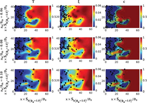
A comparison between the mixture fraction field and reaction progress variable field indicates that, almost without exception, the inhomogeneous mixture arising from evaporation remains fuel-lean (i.e., ) on the unburned gas side. The reaction progress variable fields in Figure 1 show important differences that arise due to the change of initial droplet diameter , although turbulent intensity and remain constant. It can be seen from Figure 1 that for the smallest droplets most isosurfaces lie very close together, whereas, the isosurfaces are increasingly separated from each other for the medium and large droplets, indicating a broadening of the flame in these cases.

The simulation methodology adopted here is restricted to situations where the droplet size is smaller than the Kolmogorov length scale. Thus, the simulation methodology adopted here is valid only for the external group combustion and external sheath group combustion according to the regime diagram by Chiu et al. (1982), which was discussed in detail by Reveillon and Vervisch (2000). Chiu and Liu (1977) defined a group number, (where and are the Lewis and Schmidt numbers, respectively; is the number of droplets in a specified volume; and is the mean inter-droplet distance) in order to distinguish between individually burning droplets () and external sheath combustion (). All droplet cases considered here come under the category of external group combustion (i.e., have values of much greater than unity). While Figure 1 gives an impression that individually burning droplets are present in the burned gas region, it should be noted that Figure 1 shows only one plane and that other droplets may reside in adjacent planes.

The regime of combustion can be characterized with the help of the Karlovitz number , which provides a measure of the ratio of flame thickness to the Kolmogorov length scale (Peters, 2000). For a stoichiometric mixture with values of and one obtains a Karlovitz number of 9.0, and for the values of and . Thus, the value of the Karlovitz number is likely to be large under fuel-lean conditions (since ), which suggests that combustion in all cases considered here takes place well within the thin reaction zones regime (Peters, 2000). Furthermore, the Damköhler number scales as (Peters, 2000) and, hence, low Damköhler number combustion is likely for the high Karlovitz number cases considered here. This can further be substantiated from the variation of with shown in Figure 2. According to Bray et al. (1985) one obtains: where the last term is negligible for high values of Damköhler number. It is possible to obtain maximum possible values of the variance ) where the of (i.e., ) shows a bi-modal distribution with delta functions at and , which takes the following form:

(24)

Figure 2. Variation of with across the flame brush for all turbulent droplet cases with (red), (blue), (green), and (magenta). The dashed black line shows .

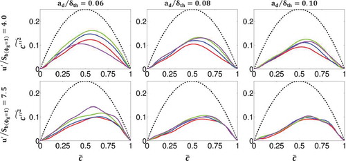
where , and are the weights associated with the PDF contributions and is the burning mode PDF, which originates from the interior of the flame. The third term on the right-hand side of Eq. (24) is of the order of (Bray et al., 1985) and thus this contribution can be ignored for . However, since the chemical reaction in the gaseous phase takes place predominantly in a fuel-lean mode for the droplet cases considered here, Da is expected to be small (due to small values of for fuel-lean mixtures), which leads to a significant departure of from in turbulent droplet cases (i.e., it is expected that departs significantly from the aforementioned bi-modal distribution). It is evident from Figure 2 that the low Damköhler number effects (i.e., effects of slow chemical reaction) are stronger for the cases with large and medium droplets and weaker for the cases with small droplets. This is once again due to the fact that smaller droplets evaporate more quickly, allowing more fuel vapor to be released than in the case of larger droplets. Similarly, the effects of increasing are less noticeable for medium and large droplets, although this does lead to slight increases in for these droplets. Whereas the effects for small droplets are much more noticeable, in most cases an increase in leads in turn to an increase in (and also faster chemical reaction) due to the extra gaseous fuel that is released. The exception being (for small droplets) where the abundance of gaseous fuel leads to fuel-rich mixture, which reduces the rate of chemical reaction.

Distributions of and and their modeling

It is often necessary to evaluate , , and for the purpose of modeling , , and in turbulent partially premixed combustion according to the following expressions (Malkeson et al., 2013; Ruan et al., 2012):

(25)

where and are the turbulent kinetic energy and its dissipation rate, respectively, and , and are the model parameters. Irrespective of the performance and validity of the expressions given by Eq. (25) for spray combustion, it is worth noting that , , and are unclosed terms and they can be expressed as:

(26a)

(26b)

(26c)

where is the Favre-PDF of a general quantity; is the mean gas density conditional on q with being the marginal PDF of q. Equations (23), (25), and (26) indicate that the knowledge of , , and is necessary in addition to the PDFs of and for the purpose of modeling , , and .

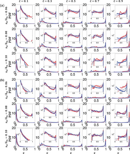
Figure 3a shows the joint of and for , which is denoted as , for the droplet cases with and under turbulent flow conditions . Although shows considerable peaks near on and near on , it is clear from Figure 3a that the distribution of departs significantly from the presumed PDF of given by Eq. (24). This is especially true for lower values of , which reside predominantly in regions of fuel-lean mixture, as has been noted with regard to Figure 1, resulting in a much slower combustion process with a low Damköhler number. This phenomenon is apparent for all droplet sizes considered here. The reason for this is that even the smallest droplets considered here are not sufficiently small to evaporate quickly enough to produce significant quantities of stoichiometric mixture on low values of Figure 3a shows that the joint PDF cannot be accurately approximated in terms of discrete delta functions throughout the flame brush as was used previously by Ribert et al. (2005), Robin et al. (2006), and Mura et al. (2007) for approximating the joint PDF between and (i.e., ). The joint PDFs between and (i.e., ) have also been found to be inadequately represented by discrete delta functions (not shown here), which is qualitatively similar to . However, the profiles of begin to show some attributes of delta functions as increases. This process occurs most rapidly for the small droplets, which evaporate more readily and, hence, are more likely to produce regions of stoichiometric mixture than larger droplets, such that on the profile of for the small droplets is confined to and a narrow band of values bounding . The larger droplets show the same trend, but due to their slower evaporation, do not resemble delta functions as much as the small droplets.

Figure 3. (a) Joint PDF between and (i.e., ) for in droplet cases with and for (left to right) droplets with normalized initial diameter and 0.10, respectively. -Axis: ; -axis: ; and -axis: . (b–c) Contours of (top) and (bottom) on (b) and (c) for one droplet case ().

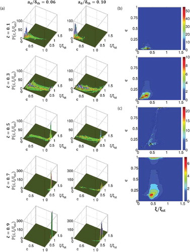
It can further be seen from Figure 3a that the peak value of the joint PDF is obtained at and for . The peak of at arises principally from the region due to the high rate of droplet evaporation as a result of the high temperature in the burned gas region. Furthermore, the peak value of is obtained at and due to the diffusion-type flame which develops as a result of droplet evaporation in the burned gas region and the subsequent back-diffusion of the evaporated fuel (Wacks et al., 2015).

The joint PDFs for the variation of and are not shown here for the sake of brevity. It can be reported, however, that as increases, for the same initial turbulent flow conditions , there is a shift in the position of the peak which is located at (on ) towards higher values of , as may be anticipated due to the extra availability of fuel in liquid form, which in turn leads to more gaseous fuel. In addition, the peak at is less well defined with the values being spread over a wider range of . As the turbulent intensity is decreased to , the joint PDFs show higher values of across due to the lack of sufficient turbulent mixing. This effect is compounded by increasing the value of and is most noticeable for small droplets, which evaporate more easily than the medium or large droplets. The relatively high likelihood of attaining signifies the development of regions in which the reaction proceeds slowly due to the fuel-rich mixture.

As was mentioned above, the evaluation of can be expressed as a function of (see Eq. (26c)). In the cases of statistical independence of and , the joint PDF can be approximated by , which would then simplify the evaluation of . Figures 3b and 3c compare the contours of and on and for a representative droplet case. The contours on higher values of are not shown as they do not provide useful information due to the sharp peak of the joint PDFs. It can be seen from Figures 3b and 3c that and are somewhat similar in appearance, but different in magnitude on these values of . However, it has already been discussed that high values of (i.e., ) are more likely for , thus it cannot be expected that and are statistically independent of each other. Accordingly, it may not be appropriate to model by for the purpose of simplifying the integral given by Eq. (26c).

The Favre-PDFs of the mixture fraction (i.e., ) are shown in Figure 4 for all droplet sizes () and for both turbulent intensities () for the lowest and highest values of droplet equivalence ratio () at several locations across the flame brush (). Figure 4 shows that the nature of the Favre-PDFs varies significantly with position in the flame and that in all cases shown here the most likely mixture shifts from fuel-lean on the unburned gas side () to stoichiometric (/fuel-rich on the burned gas side (). In the mid-region (), the progression from fuel-lean to stoichiometric/fuel-rich is achieved most swiftly by the smaller droplets due to a higher rate of evaporation, whereas larger droplet cases remain fuel-lean for a greater range of . Furthermore, the Favre-PDFs of for cases with lower turbulence intensity (), although very often following closely the Favre-PDFs of the cases with higher turbulence intensity () both in shape and magnitude, show consistently a higher probability of a more fuel-lean mixture at most locations in the flame. The noteable exception to this is for small droplets at the higher droplet equivalence ratio (). Under these conditions, the abundance of small droplets evaporate quickly and are not mixed sufficiently well by the flow of lower turbulent intensity, giving rise to a greater likelihood of fuel-rich regions than for the higher turbulent intensity, which is strong enough to mix the evaporated fuel. In general, the higher droplet equivalence ratio () gives rise to a greater spread of values of than the lower droplet equivalence ratio () and, in particular, to non-negligible probabilities of attaining fuel-rich mixtures. This phenomenon arises naturally from the higher probability of droplets being in closer proximity (due to higher droplet number density) for higher droplet equivalence ratios, thereby giving rise to higher concentrations of gaseous fuel, despite the effects of turbulent mixing. In order to model the Favre-PDF of , a presumed -function PDF approach is often considered in the context of single gaseous phase combustion (Poinsot and Veynante, 2001). The -function PDF of a scalar is defined as:

(27)

Figure 4. Comparison of Favre-PDFs of normalized mixture fraction (i.e., ) at (left to right) for all droplet cases with (a) and (b) with (red) and (blue) showing DNS data (solid lines) and -function (dashed lines).

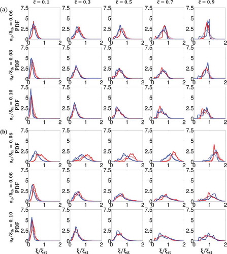
where is a normalization factor with and . Figure 4 shows that the assumption reasonably captures the general shape and magnitude of the Favre-PDFs obtained from the DNS data.

Indeed, the agreement of the -function PDF with is consistent with the modeling assumptions made by Sadiki et al. (2012) and Ma et al. (2014) in the context of FGM-based simulations of turbulent spray combustion. However, it must be emphasized that the use of the -function PDF to model may not be suitable in all cases of droplet combustion, as has already been shown by Ge and Gutheil (2006) and Luo et al. (2011). Ge and Gutheil (2006) proposed a modification to the standard -function PDF: , where and refer to maximum and minimum values of , which has recently been used by Tyliszczak et al. (2014) for LES of spray combustion. It is also worth noting that Borghesi et al. (2011) parameterized in terms of the -function PDF in the context of CMC modeling and assumed that can be approximated as a -function PDF when the variance of mixture fraction is greater than a threshold limit given by: when and is considered to be (see Eq. (13)), whereas can be considered to be zero (Tyliszczak et al., 2014). In order words, the modified -function PDF proposed by Ge and Gutheil (2006) (i.e., ) reduces to Eq. (27) for small magnitudes of and . In the cases considered here the magnitude of well below unity (i.e., ) within the flame brush for n-heptane combustion and, thus, the standard -function PDF predicts satisfactorily for the cases considered here. However, Eq. (27) may not be sufficient for a different fuel and flow conditions where is much smaller than unity.

Figure 5 shows the Favre-PDFs of (i.e., ) for all droplet sizes () and for both turbulent intensities () for the lowest and highest values of droplet equivalence ratio () at several locations across the flame brush (). All locations in the flame shown here exhibit an almost monomodal distribution. On it is most likely to achieve a value . This is reflected to some extent on , where the most likely outcome is slightly greater than . In contrast, on it is most likely to achieve a value , with the likelihood increasing as increases from to . The likelihood of achieving a value on is greater for small droplets than for large droplets. This feature is reversed on , where the likelihood of achieving is greater for large droplets than for small droplets. This is true at both values of droplet equivalence ratio shown here and for both values of turbulent intensity. It is clear from Figure 5 that the Favre-PDF of cannot be approximated by Eq. (24), whereas the -function PDF (see Eq. (27)) parameterized in terms of and (i.e., with and ) has been found to reasonably capture the general shape and magnitude of the reaction progress variable Favre-PDFs obtained from DNS data. This is consistent with the modeling assumption made by Ma et al. (2014) in the context of FGM based modeling of turbulent spray combustion. It is worth noting a number of analyses on single-phase homogeneous (Ahmed and Swaminathan, 2013; Kolla and Swaminathan, 2010) and inhomogeneous (Chen et al., 2015; Ruan et al., 2014) mixture combustion used -function PDF for parameterising in the past.

Figure 5. Comparison of Favre-PDFs of reaction progress variable (i.e., ) at (left to right) for all droplet cases with (a) and (b) with (red) and (blue) showing DNS data (solid lines) and -function (dashed lines). Insets show log-linear plots.

Statistical behavior and the modeling of the PDFs of and

Figures 6 and 7 show the PDFs of and , respectively. Often a presumed log-normal distribution is used to model these PDFs. The log-normal distribution of a scalar, , is given by:

(28)

Figure 6. Comparison of PDFs of normalized mixture fraction gradient across the flame brush between DNS data (solid lines) and lognormal distribution (dashed lines) at (red-green-blue-magenta-cyan) for droplet sizes (left to right) at with (a) and (b) .

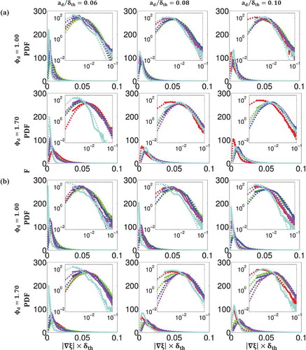
Figure 7. Comparison of PDFs of normalized reaction progress variable gradient across the flame brush between DNS data (solid lines) and lognormal distribution (dashed lines) at (red-green-blue-magenta-cyan) for droplet sizes (left to right) at with (a) and (b) .

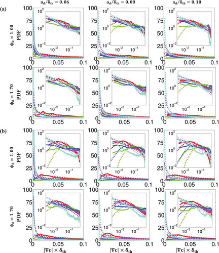
where and are mean and standard deviation of the natural logarithm of . Figures 6 and 7 show that both qualitatively and quantitatively the log-normal distribution succeeds in capturing the PDFs of the DNS data for all values of , and . The only exception takes place at high values of and where there is insufficient data in the DNS dataset to accurately predict the value of the PDF and the regions with high probability of finding , which log-normal distribution fails to predict. The discrepancy between the log-normal distribution and the tail of the scalar gradient PDFs is consistent with several experimental (Geyer et al., 2005; Karpetis and Barlow, 2002; Markides and Mastorakos, 2006; Sreenivasan and Antonia, 1997; Su and Clemens, 2003) and computational (Hawkes et al., 2007; Knaus et al., 2012; Malkeson et al., 2013; Pantano, 2004; Ruan et al., 2012) findings in the context of passive scalar mixing, non-premixed, and partially-premixed combustion. Despite some inaccuracies, the log-normal distribution appears to do a reasonable job for the purpose of parameterising and , which in turn could be used for modeling the scalar dissipation rates and .

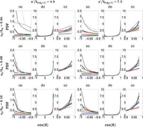
Interrelation between and

It is important to understand the relative alignment between and so that the scalar inner product of and (i.e., ) can be parameterized in terms of and in Eq. (23c) for the purpose of evaluating (and ). The relative alignment between and can be quantified in terms of the angle between and :

(29)

A distinction may be drawn between flames in partially-premixed mixtures where the flame-front is propagating towards a leaner mixture, also known as back-supported flames, and where the flame-front is propagating towards a richer mixture, also known as front-supported flames. Hence, it follows that front-supported flames arise when the signs of and are opposite to each other and back-supported flames arise when and possess the same sign. According to Eq. (29), implies the presence of front-supported flames and implies the presence of back-supported flame-fronts. Figure 8 shows the PDFs of for all droplet sizes () and for both turbulent intensities () for the lowest and highest values of droplet equivalence ratio () on several -isosurfaces across the flame front (). The PDFs of for are also shown. It is apparent from the PDFs of the entire range of (i.e., subplot (b)) that in most droplet cases, although there is a non-negligible probability of finding front-supported flames, back-supported flames are far more likely to be found. This is consistent with the observation that can be made from Figure 1, which shows, based on the comparison of and fields, that flame predominantly propagates into fuel-lean mixture and thus positive values of principally contribute to the evaluation of (and ) according to Eq. (23c). The likelihood of back-supported flames increases significantly with increasing droplet size and with increasing turbulent intensity, whereas the likelihood of front-supported flames is largely unaffected by increases in either droplet size or turbulent intensity. The only exception to this trend can be seen in cases of small droplets with high droplet equivalence ratio and under low turbulent intensity: conditions, which give rise to the greatest inhomogeneities, due to the rapid evaporation of a large number of small droplets combined with a lack of turbulent mixing. Also included in Figure 8 are the subplots that focus on the peak values (i.e., subplot (a)) and (i.e., subplot (c)). These subplots show that, for small droplets, it is the -isosurfaces towards the burned gas side (e.g., under initial and under initial ) that are most likely to produce front-supported flames for due to relatively large amounts of evaporated fuel vapor, whereas for medium and large droplets, it is the unburned gas side (e.g., isosurface), which exhibits the high probability of finding front-supported flames because of localized islands of fuel-rich zones arising from evaporation on the unburned gas side of the flame front. Conversely, the -isosurfaces on the burned gas side (e.g., ) are most likely to produce back-supported flames in most droplet cases due to the predominantly fuel-lean nature of the unburned gas of the flame front, except for small droplets under low initial turbulence intensity, for which the unburned gas side (e.g., ) is most likely to exhibit back-supported flames because of greater probability of finding richer mixture on burned gas side in these cases due to conducive conditions for higher evaporation rate.

Figure 8. PDFs of for all (black) and for (red-green-blue-magenta-cyan) in droplet cases with (solid lines) and (dashed lines) with (left to right columns) for (top to bottom rows) droplets with normalized initial diameter , 0.08, and 0.10, respectively. Sub-figures: (a) close-up of LHS of range, (b) entire range, and (c) close-up of RHS of range.

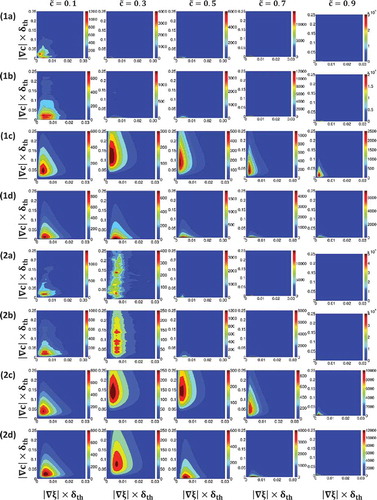
Finally, Figure 9 shows joint PDFs of and , , and across the flame brush for several droplet cases (, , ). Other cases display the same qualitative behavior and thus are not shown here in the interest of conciseness. No clear correlation is apparent between and , which is consistent with a previous analysis (Malkeson et al., 2013; Ruan et al., 2012). Although the absence of correlation does not necessarily mean statistical independence, the similarity between and suggests that statistical independence of and might be a valid assumption for these flames, and that the joint PDF can be modeled as . It should be noted that the discrepancies in the magnitude of the joint PDFs follow naturally from the definition of joint PDFs (i.e., that the volume under the joint PDF equals unity), with the result that minor differences in spread of the joint PDFs can give rise to noticeable differences in their magnitudes.

Figure 9. Contours of P() (Row 1), (Row 2), lognormal bivariate distribution of and assuming correlation (row 3) and assuming no correlation (row 4) at 1, 0.3, 0.5, 0.7, 0.9 for droplets of size and where (rows 1a–1d) and (rows 2a–2d) .

The modeling of the joint PDF is often considered using the bi-variate distribution (Abramowitz and Stegun, 1970; Malkeson et al., 2013; Ruan et al., 2012; Yerel and Konuk, 2009), which takes the following form:

(30a)

where and are random variables with means (standard deviations) and ( and ), and is the correlation coefficient, which is given by:

(30b)

where indicates the expected value of a given variable and is given as:

(30c)

It is worth noting that the correlation coefficient becomes zero when the random variables and are statistically independent. Under such conditions, the bi-variate distribution takes the following form:

(30d)

Figure 9 also compares the predictions of Eqs. (30a) and (30d) with extracted from DNS data for several droplet cases (, , ). Other cases display the same qualitative behavior and thus are not presented here for the sake of brevity.

A comparison between Figure 9a and Figures 9c–9d reveals slightly better agreement between the joint PDF obtained from DNS data and the lognormal bivariate distribution without correlation (i.e., Eq. (30d)) than the predictions of Eq. (30a), which accounts for the correlation between and . The better agreement is apparent only at intermediate values of (i.e., ) for which the spread of the lognormal bivariate distribution without correlation is smaller than the corresponding spread with correlation, which more closely matches the spread of the joint PDF. The degree of similarity between Figures 9c and 9d depends on the specific value of the correlation coefficient, , in each case, such that cases where the correlation coefficient is small, Figures 9c and 9d appear similar, since under such circumstances Eq. (30a) reduces to Eq. (30d). Thus, it may be said that the bivariate lognormal distribution with correlation better approximates the joint PDF when the correlation coefficient is small. In other words, the joint PDF may be better approximated by the bivariate lognormal distribution without correlation. This is consistent with the findings from Figures 9a and 9b, which indicate that can be approximated by because the approximation implicitly assumes statistical independence and thus zero correlation between and . The statistical independence between and is also implicitly assumed in the derivation of Eq. (30d). As log-normal distribution reasonably models and (see Figures 4 and 5), the prediction of Eq. (30d) also behaves qualitatively similarly to that of extracted from DNS data. Figures 4 and 5 show that log-normal distributions do not adequately capture the tails of the PDFs of and , and thus there are quantitative differences between the predictions of Eq. (30d) and . A similar behavior was reported earlier in the context of single phase gaseous partially-premixed combustion (Malkeson et al., 2013; Ruan et al., 2012). It is worth noting that the correlation coefficient provides a measure of linear dependence between the variables in question and thus the prediction of Eq. (30a), which explicitly accounts for the correlation coefficient between and , does not necessarily capture the significantly nonlinear relation between these quantities. Thus, based on the evidence presented in Figure 9 the bi-variate log-normal distribution without correlation (i.e., Eq. (30d)) seems to be slightly better suited for modeling than the bi-variate log-normal distribution with correlation (i.e., Eq. (30a)).

Conclusions

The effects of droplet size, droplet equivalence ratio and turbulence intensity on the statistical properties of the scalars and and their gradients, and , in statistically planar flames propagating into a liquid fuel droplet mist under decaying turbulence have been analyzed using modified simple chemistry (Tarrazo et al., 2006) 3D DNS data. The combustion process in the gaseous phase has been found to take place predominantly in fuel-lean mode, even for , nevertheless droplets which were able to penetrate the flame front completed their process of evaporation in the burned gas region, releasing gaseous fuel which, by means of diffusion, increased the gaseous equivalence ratio in the region of the flame front. The probability of finding fuel-lean mixture decreases with decreasing initial droplet diameter due to faster evaporation of smaller droplets. An increase in droplet equivalence ratio also reduces the probability of having fuel-lean combustion, whereas an increase in encourages the mixing of evaporated fuel with surrounding air and produces a more flammable mixture, which plays a crucial role for small droplets at high values of . It was shown that the joint PDF of and cannot, in many cases, be accurately modeled in terms of discrete delta functions, and its magnitudes cannot be predicted by ) due to statistical dependence between and at some locations within the flame. It has further been shown that a -function distribution reasonably predicts the shape and magnitude of the Favre-PDFs of and c. A presumed log-normal distribution captures both qualitative and quantitative behaviors of the PDFs of and obtained from the DNS data across the flame brush, but there exist discrepancies between the log-normal distribution and DNS data at the tails of the PDFs. The PDFs of cosine of the angle between and (i.e., ) have been found to exhibit much greater likelihood of positive values than negative values for most droplet cases. This phenomenon arises due to the predominantly fuel-lean nature of the unburned gas region of the flame. A greater probability of negative values of has been observed in cases of small droplet than in cases of larger droplets and detailed explanations for this behavior have been provided. It has been found that the joint PDF of and (i.e., ) can be approximated by P(, which implicitly assumes statistical independence of and . Two variants of bivariate log-normal distribution have been considered for the purpose of modeling , assuming both correlation and no correlation between and . Significant quantitative discrepancies have been found between obtained from DNS data and the predictions of the parameterization based on bivariate log-normal distribution, which originate principally due to inaccuracies incurred during parameterising P( and P(by log-normal distributions. The variant with no correlation has been found to be more successful in capturing qualitative behavior of than the variant which accounts for correlation between and . It is worth noting that the present analysis has been carried out for modified single step chemistry (Tarrazo et al., 2006) DNS data with moderate values of turbulent Reynolds number and thus experimental and detailed chemistry DNS data at high values of turbulent Reynolds numbers will be necessary for more comprehensive analysis and validation of the parameterizations, which have been found to exhibit the most promising behavior when compared to DNS data. Furthermore, the aforementioned parameterizations need to be implemented in actual RANS and LES simulations for the purpose of a-posteriori assessment.

Acknowledgments

The computational resources of N8 and ARCHER are gratefully acknowledged. The authors are also grateful to Prof. E. Mastorakos for his invaluable advice.

Funding

The authors gratefully acknowledge the financial assistance of EPSRC (EP/J021997/1 and EP/K025163/1).

Additional information

Funding

The authors gratefully acknowledge the financial assistance of EPSRC (EP/J021997/1 and EP/K025163/1).

References

- Abramowitz, M., and Stegun, I.A. (Eds.). 1970. Handbook of Mathematical Functions, Dover, New York.
- Aggarwal, S.K. 1998. A review of spray ignition phenomena: Present status and future research. Prog. Energy Combust. Sci., 24, 565.
- Aggarwal, S.K., and Sirignano, W.A. 1985. Unsteady spray flame propagation in a closed volume. Combust. Flame, 62, 69.
- Ahmed, I., and Swaminathan, N. 2013. Simulation of spherically expanding turbulent premixed flames, Combust. Sci. Technol., 185, 1509.
- Ballal, D.R., and Lefebvre, A.H. 1981. Flame propagation in heterogeneous mixtures of fuel droplets, fuel vapour and air. Proc. Combust. Inst., 18, 312.
- Borghesi, G., Mastorakos, E., Devaud, C.B., and Bilger, R.W. 2011. Modelling evaporation effects in conditional moment closure for spray autoignition. Combust. Theor. Model., 15, 725.
- Bray, K., Libby, P., and Moss, J. 1985. Unified modelling approach for premixed turbulent combustion—Part 1: General formation. Combust. Flame, 61, 87.
- Bray, K.N.C., Domingo, P., and Vervisch, L. 2005. Role of the progress variable in models for partially premixed turbulent combustion. Combust. Flame, 141, 431.
- Burgoyne, J.H., and Cohen, L. 1954. The effect of drop size on flame propagation in liquid aerosols. Proc. R. Soc. London, Ser. A, 225, 375.
- Chen, Z., Ruan, S., and Swaminathan, N. 2015. Simulation of turbulent lifted methane jet flames: Effects of air-dilution and transient flame propagation. Combust. Flame, 162, 703.
- Chiu, H.H., Kim, H.Y., and Croke, E.J. 1982. Internal group combustion of liquid droplets. Proc. Combust. Inst., 19, 971.
- Chiu, H.H., and Liu, T.M. 1977. Group combustion of liquid droplets. Combust. Sci. Technol., 17, 127.
- Clift, R., Grace, J.R., and Weber, M.E. 1978. Bubbles, Drops, and Particles, Academic Press, New York.
- Faeth, G.M. 1987. Mixing, transport and combustion sprays. Prog. Energy Combust. Sci., 13, 293.
- Fujita, A., Watanabe, H., Kurose, R., and Komori, S. 2013. Two-dimensional direct numerical simulation of spray flames—Part 1: Effects of equivalence ratio, fuel droplet size and radiation, and validity of flamelet model. Fuel, 104, 515.
- Ge, H.-W., and Gutheil, E. 2006. PDF simulation of turbulent spray flows. Atomization Sprays, 16(5), 531.
- Geyer, D., Kempf, A., Dreizler, A., and Janicka, J. 2005. Scalar dissipation rates in isothermal and reactive turbulent opposed-jets: 1-D Raman/Rayleigh experiments supported by LES. Proc. Combust. Inst., 30, 681.
- Greenberg, J.B., Kagan, L.S., and Sivashinsky, G. 2009. Stability of rich premixed spray flames. Atomization Sprays, 19, 863.
- Greenberg, J.B., Silverman, I., and Tambour, Y. 1998. On droplet enhancement of the burning velocity of laminar premixed spray flames. Combust. Flame, 113, 271.
- Hawkes, E., Sankaran, R.R., Sutherland, J.C., and Chen, J.H. 2007. Scalar mixing in direct numerical simulations of temporally evolving plane jet flames with skeletal CO/H2 kinetics. Proc. Combust. Inst., 31, 1633.
- Hayashi, S., Kumagai, S., and Sakai, T. 1976. Propagation velocity and structure of flames in droplet-vapor-air mixtures. Combust. Sci. Technol., 15, 169.
- Heywood, J.B. 1998. Internal Combustion Engine Fundamentals, 1st ed., McGraw Hill, New York.
- Jenkins, K.W., and Cant, R.S. 1999. Direct numerical simulation of turbulent flame kernels. In Recent Advances in DNS and LES: Proceedings of the Second AFOSR Conference, D. Knight and L. Sakell (Eds.), Rutgers –The State University of New Jersey, New Brunswick, NJ, June 7–9; Kluwer Academic Publishers, New York, pp. 192–202.
- Karpetis, A.N., and Barlow, R.S. 2002. Measurements of scalar dissipation in a turbulent piloted methane/air jet flame. Proc. Combust. Inst., 29, 1929.
- Knaus, R., Oefelein, J., and Pantano, C. 2012. On the relationship between the statistics of the resolved and the true rate of dissipation of mixture fraction. Flow Turbul. Combust., 89, 37.
- Kolla, H., and Swaminathan, N. 2010. Strained flamelets for turbulent premixed flames, I: formulation and planar flame results. Combust. Flame, 157, 943.
- Kuo, K., and Acharya, R. 2012. Fundamentals of Turbulent and Multi-Phase Combustion, 2nd ed., Wiley, Hoboken, NJ.
- Lawes, M., and Saat, A. 2011. Burning rates of turbulent iso-octane aerosol mixtures in spherical flame explosions. Proc. Combust. Inst., 33, 2047.
- Lefebvre, A.H. 1998. Gas Turbine Combustion, 2nd ed., Taylor & Francis, Ann Arbor, MI.
- Luo, K., Pitsch, H., Pai, M.G., and Desjardins, O. 2011. Direct numerical simulations and analysis of three-dimensional n-heptane spray flames in a model swirl combustor. Proc. Combust. Inst., 33, 2143.
- Ma, L., Naud, B., and Roekaerts, D.J.E.M. 2014. Modeling ethanol spray jet flame in hot-diluted coflow with transported pdf. Presented at SPEIC2014—Towards Sustainable Combustion, Lisboa, Portugal, November 19–21.
- Malkeson, S.P., and Chakraborty, N. 2010. Statistical analysis of displacement speed in turbulent stratified flames: A direct numerical simulation study. Combust. Sci. Technol., 182, 1841.
- Malkeson, S.P., Ruan, S., Chakraborty, N., and Swaminathan, N. 2013. Statistics of reaction progress variable and mixture fraction gradients from DNS of turbulent partially premixed flames. Combust. Sci. Technol., 185, 1329.
- Markides, C.N., and Mastorakos, E. 2006. Measurements of scalar dissipation in a turbulent plume with laser planar induced fluorescence of acetone. Chem. Eng. Sci., 61, 2835.
- Miller, R.S., and Bellan, J. 1999. Direct numerical simulation of a confined three-dimensional gas mixing layer with one evaporating hydrocarbon-droplet-laden stream. J. Fluid Mech., 384, 293.
- Mura, A., Robin, V., and Champion, M. 2007. Modeling of scalar dissipation in partially premixed turbulent flames. Combust. Flame, 149, 217.
- Nakamura, M., Akamatsu, F., Kurose, R., and Katsuki, M. 2005. Combustion mechanism of liquid fuel spray in a gaseous flame. Phys. Fluids, 17, 123301.
- Neophytou, A., and Mastorakos, E. 2009. Simulations of laminar flame propagation in droplet mists. Combust. Flame, 156, 1627.
- Neophytou, A., Mastorakos, E., and Cant, R.S. 2010. DNS of spark ignition and edge flame propagation in turbulent droplet-laden mixing layers. Combust. Flame, 157, 1071.
- Neophytou, A., Mastorakos E., and Cant, R.S. 2011. Complex chemistry simulations of spark ignition in turbulent sprays. Proc. Combust. Inst., 33, 2135.
- Neophytou, A., Mastorakos E., and Cant, R.S. 2012. The internal structure of igniting turbulent sprays as revealed by complex chemistry DNS. Combust. Flame, 159, 641.
- Nomura, H., Koyama, M., Miyamoto, H., Ujiie, Y., Sato, J., Kono, M., and Yoda, S. 2000. Microgravity experiments of flame propagation in ethanol droplet-vapor-air mixture. Proc. Combust. Inst., 28, 999.
- Pantano, C. 2004. Direct simulation of non-premixed flame extinction in a methane-air jet with reduced chemistry. J. Fluid Mech., 514, 231.
- Peters, N. 2000. Turbulent Combustion, Cambridge University Press, Cambridge, UK.
- Poinsot, T.J., and Lele, S. 1992. Boundary conditions for direct simulations of compressible viscous flows. J. Comput. Phys., 101, 104.
- Poinsot, T., and Veynante, D. 2001. Theoretical and Numerical Combustion, R.T. Edwards Inc., Philadelphia, PA.
- Reveillon, J., and Demoulin, F.X. 2007. Evaporating droplets in turbulent reacting flows. Proc. Combust. Inst., 31, 2319.
- Reveillon, J., and Vervisch, L. 2000. Spray vaporization in non-premixed turbulent combustion modelling: A single droplet model. Combust. Flame, 121, 75.
- Ribert, G., Champion, M., Gicquel, O., Darabiha, N., and Veynante, D. 2005. Modeling of nonadiabatic turbulent premixed reactive flows including tabulated chemistry. Combust. Flame, 141, 271.
- Robin, V., Mura, N., Champion, M., and Plion, P. 2006. A multi-Dirac presumed PDF model for turbulent reacting flows with variable equivalence ratio. Combust. Sci. Technol., 178, 1843.
- Rogallo, R.S. 1981. Numerical experiments in homogeneous turbulence. NASA Technical Memorandum 81315. NASA Ames Research Center, Moffett Field, CA.
- Ruan, S., Swaminathan, N., Bray, K.N.C., Mizobuchi, Y., and Takeno, T. 2012. Scalar and its dissipation in the near field of turbulent lifted jet flame. Combust. Flame, 159(2), 591.
- Ruan, S., Swaminathan, N., and Darbyshire, O. 2014. Modelling of turbulent lifted jet flames using flamelets: A priori assessment and a posteriori validation. Combust. Theor. Model., 18, 295.
- Sadiki, A., Chrigui, M., and Dreizler, A. 2012. Thermodynamically consistent modelling of gas turbine combustion sprays. In J. Janicka, A. Sadiki, M. Schäfer, and C. Heeger (Eds.), Flow and Combustion in Advanced Gas Turbine Combustors, Springer, Netherlands.
- Silverman, I., Greenberg, J.B., and Tambour, Y. 1993. Stoichiometry and polydisperse effects in premixed spray flames. Combust. Flame, 93, 97.
- Sreedhara, S., and Huh, K.Y. 2007. Conditional statistics of nonreacting and reacting sprays in turbulent flows by direct numerical simulation. Proc. Combust. Inst., 31, 2335.
- Sreenivasan, K.R., and Antonia, R.A. 1997. The phenomenology of small-scale turbulence. Annu. Rev. Fluid Mech., 29, 435.
- Su, L.K., and Clemens, N.T. 2003. The structure of fine-scale scalar mixing in gas-phase planar turbulent jets. J. Fluid Mech., 488, 1.
- Szekely, Jr., G.A., and Faeth, G.M. 1983. Effects of envelope flames on drop gasification rates in turbulent diffusion flames. Combust. Flame, 49, 255.
- Tarrazo, E., Sanchez, A., Linan, A., and Williams, F.A. 2006. A simple one-step chemistry model for partially premixed hydrocarbon combustion. Combust. Flame, 147, 32.
- Tyliszczak, A., Cavaliere, D.E., and Mastorakos, E. 2014. LES/CMC of blow-off in a liquid fueled swirl burner. Flow Turbul. Combust., 92, 237.
- Wacks, D.H., Chakraborty, N., and Mastorakos, E. 2015. Statistical analysis of turbulent flame-droplet interaction: A direct numerical simulation study. Flow Turbul. Combust., 96, 573–607.
- Wandel, A. 2013. Extinction predictors in turbulent sprays. Prog. Combust. Inst., 34(1), 1625.
- Wandel, A. 2014. Influence of scalar dissipation on flame success in turbulent sprays with spark ignition. Combust. Flame, 161, 2579.
- Wandel, A., Chakraborty, N., and Mastorakos, E. 2009. Direct numerical simulation of turbulent flame expansion in fine sprays. Proc. Combust. Inst., 32, 2283.
- Wang, Y., and Rutland, C.J. 2005. Effects of temperature and equivalence ratio on the ignition of n-heptane fuel spray in turbulent flow. Proc. Combust. Inst., 30, 893.
- Watanabe, H., Kurose, R., Hwang, S.-M., and Akamatsu, F. 2007. Characteristics of flamelets in spray flames formed in a laminar counterflow. Combust. Flame, 148, 234.
- Watanabe, H., Kurose, R., Komori, S., and Pitsch, H. 2008. Effects of radiation on spray flame characteristics and soot formation. Combust. Flame, 152, 2.
- Wray, A.A. 1990. Minimal storage time advancement schemes for spectral methods, Unpublished report. NASA Ames Research Center, Moffett Field, CA.
- Xia, J., and Luo, K.H. 2010. Direct numerical simulation of inert droplet effects on scalar dissipation rate in turbulent reacting and non-reacting shear layers. Flow. Turbul. Combust., 84, 397–422.
- Yerel, S., and Konuk, A. 2009. Bivariate lognormal distribution model of cutoff grade impurities: A case study of magnesite ore deposit. Sci. Res. Essay, 4(12), 1500.