Two-dimensional measurements of soot in a turbulent diffusion diesel flame: the effects of injection pressure, nozzle orifice diameter, and gas density

ABSTRACT

Two-dimensional light extinction, flame luminosity, and OH* chemiluminescence images were captured at a constant ambient temperature of 823 K and two gas densities (20 and 26 kg/m³), with injection pressures of 800–2500 bar using nozzle orifices with diameters of 0.19 and 0.10 mm. Soot volume fraction and OH distribution images were obtained using the Abel inversion method, and the local equivalence ratio in the lift-off length region was predicted. The results show that the equivalence ratio along the jet’s center at the lift-off length () was found to play a critical role in soot formation. Reductions in thickened the OH zone in the upstream region of the jet, reducing the volume corresponding to the maximum soot volume fraction. The expansion of the OH zone also helped reduce the sooting zone’s width. Under high sooting conditions (e.g., >3.5), the sooting zone width in the downstream jet was independent of .

KEY WORDS:

• Diesel spray
• Soot formation and oxidation
• Laser extinction
• OH* Chemiluminescence
• Local equivalence ratio

1. Introduction

In a conventional compression-ignited combustion engine, the combustion process that occurs after the end of the premixed combustion phase is that of a typical lifted turbulent diffusion flame. The combustion characteristics during this phase are strongly affected by several operating parameters. In early studies, Pickett and Siebers (2002, 2004, 2005) showed that soot formation in reacting diesel jets was reduced by reducing the nozzle orifice diameter or increasing the injection pressure. They concluded that the reduction in soot formation correlated with the reduction of the cross-sectionally averaged equivalence ratio at the lift-off length. They also found that the optical path length (i.e., the sooting zone width) was independent of the injection pressure (Pickett and Siebers, 2004). This contradicted our earlier report (Du et al., 2017) stating that the width of sooting zone decreased as the injection pressure increased at moderately sooting conditions. We found that the contribution of reduced soot formation in the radial direction correlated with an increase in the thickness of the OH radical zone and a reduction in the local equivalence ratio in the region around the lift-off length. These conclusions are consistent with the recent findings of Maes et al. (2016), who reported that the thickness of the OH radical-containing region increased with the injection pressure. The difference between our previous findings (Du et al., 2017) and those of Pickett and Siebers (2004) may be due to the use of different experimental conditions. We recently reported a study (Du et al., 2017) in which time-resolved two-dimensional light extinction and OH* chemiluminescence (henceforth referred to as OH* CL for brevity) images were captured, making it possible to observe the development of reacting diesel jets in detail. The experimental findings in that report (Du et al., 2017) were only based on a fixed nozzle outlet diameter of 0.14 mm and a fixed ambient gas density, at which the soot concentrations were relatively low. The objective of this work is to further explore the correlation between reduced soot formation in the radial direction and increased OH radical zone width under the higher/lower soot concentration conditions. To do this, experiments were carried out with a larger nozzle orifice diameter (0.19 mm) and a smaller one (0.10 mm), various injection pressures and the gas density was varied.

2. Experimental apparatus

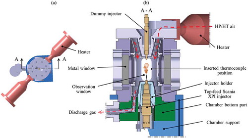
A continuous-gas-flow high-pressure/high-temperature (HP/HT) chamber was used in this work. A schematic of the spray chamber is shown in Figure 1. As can be seen in the cross-section view in Figure 1(b), the pressurized air from a compressor flows through the two 15 kW heaters, in which the air can be heated up to 900 K. The injector was mounted in the bottom of the spray chamber as shown in Figure 1(b). The velocity of air flow was controlled to be less than ~ 1 m/s, which is much smaller than the velocity of the injected fuel. Thus, the conditions inside the spray chamber can be considered as quasi-steady; a detailed description of the chamber can be found in previous reports (Du et al., 2016, 2017). In all experiments, the ambient temperature was held at 823 K ± 10 K. Two different gas densities (20 and 26 kg/m³) were employed, corresponding to a relatively low-load condition in a heavy-duty diesel engine. The chamber pressure was held within ±1 bar of the target ambient pressure. The fuel was commercial MK1 diesel fuel sold in Sweden with no added rapeseed methyl ester (RME). The chamber was fitted with a Scania XPI common rail fuel injection system and a top-feed XPI injector with axial single-hole nozzles. The injection pressure was maintained within 10 bar of the target value, and a top-flat injection rate profile was used. The experimental conditions are summarized in Table 1. It should be noted that the actual injection duration, which was determined by high-speed laser extinction imaging, was >4 ms for all operating conditions even though the energizing pulse duration was set to 3.0 ms.

Table 1. Experimental conditions.

Ambient temperature () [K]	823
Ambient pressure () [bar]	47.5, 60
Gas density () [kg/m^3]	20, 26
Oxygen concentration [%]	21
Injection pressure () [bar]	800–2500
Injection pulse [ms]	3.0
Number of injections	≥30
Frequency of injection [Hz]	~0.1
Fuel properties:
Fuel type	MK1
Density at 15°C [kg/m^3]	823.8
Cetane number	52.0
Sulfur content [mg/kg]	<2
Net heat of combustion [MJ/kg]	43.1
Total aromatics [vol%]	5.5
Nozzles:
K-factor	0
Hydro-grinding [%]	30
Length of nozzle hole [mm]	1.1
Outlet diameter (N19) [mm]	0.19
Outlet diameter (N10) [mm]	0.10

Figure 1. Top-view of the spray chamber with a small scale (a) and section view of the spray chamber with a larger scale (b).

3. Diagnostics and measurements

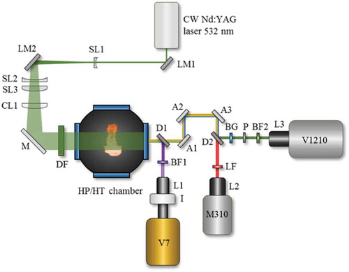
The time-resolved two-dimensional laser extinction was used to measure the soot concentration in the reacting diesel jets. In the early study by Nakakita et al. (1990), they applied two-dimensional laser extinction measurement under diesel engine-like conditions using an Ar-ion laser with wavelength of 514.5 nm. Recently, Manin et al. (2013) used an ultra-fast LED light source to capture time-resolved two-dimensional sooting images. In addition, they combined an engineered diffuser with a Fresnel lens to create an intensity distribution in the illumination background as close to Lambertian as possible, to minimize the beam steering effects. In this study, a continuous wave Nd:YAG 532 nm laser with a power of ~1.5 W was used as the light source to have a very narrow illumination spectrum. As the schematic of the optical setup in Figure 2 shows, we used a combination of positive and negative lenses to achieve a relatively uniform illumination in the observation area (i.e., sooting spray region), and a 120 grit ground glass diffuser was applied to reduce the beam-steering effects. Still, beam-steering effects could not be completely avoided, and the induced uncertainty in the soot concentration measurement will be discussed in the “Light extinction image process” section. The diffused laser light passed through the jets, and the resulting light extinction images were captured using a Phantom V1212 high-speed video CMOS camera. As shown in Figure 2, a BG39 filter, a polarizer, and a narrow bandpass filter transmitting 532 ± 1.5 nm were placed in front of the V1212 to reduce the flame luminosity as much as possible. This reduced the contribution of sooting flame luminosity in the light extinction images to <1% of the background laser light intensity even in the jet’s most intensely sooting regions (KL factor > 3.5). Natural flame luminosity (or soot luminosity) images were captured by a Phantom M310 CMOS camera, with an OG570 long-pass filter in front of it, simultaneously with light extinction images. The flame luminosity images were captured to clearly determine sooting regions in the light extinction images, since light attenuation was not only caused by soot particles, but also by the liquid fuel and to some extents by beam steering. Time-resolved two-dimensional OH* CL images were captured by a Phantom V7 camera with an image intensifier, Hamamatsu C9548. A bandpass filter transmitting 307 ± 5 nm was used to selectively transmit OH* CL. It is well established that such OH* CL images can be used to measure lift-off lengths. In addition, Maes et al. (2016) recently showed that Abel inversion of averaged OH* CL images revealed the same qualitative trends as those detected by OH planar laser-induced fluorescence (OH-PLIF). We therefore performed Abel inversion of averaged OH* CL images to characterize the distribution of OH radicals, which can be used to explain the evolution of soot in reacting diesel jets. The exposure times for the M310 and V1210 cameras were 1 µs, and their spatial resolutions were 3.77 pixels/mm and 3 pixels/mm, respectively. The gain and the gate time (20 µs) for the intensifier was constant for all experiments. The spatial resolution for the V7 camera was 4.3 pixel/mm. All cameras were synchronized using a Stanford Research Systems signal generator and had a frame rate of 27,000/s.

Figure 2. Schematic of the optical setup. LM1-2: laser line mirror at 532 nm and 45°, SL1: spherical lens (SL), focus length (fl) = −50 mm, antireflection coated, SL2: fl = −125 mm, antireflection coated, SL3: fl = + 500 mm, antireflection coated, CL1: cylindrical lens, fl = + 500 mm, M: aluminum mirror, DF: 120 grit ground glass diffuser, D1: dichroic mirror (DM) with ≥ 98% reflectance at 308 nm, D2: DM with >95% reflectance at 500–560 nm, A1-A3: aluminum mirrors, BF1: bandpass filter (BF) 307 ± 10 nm, LF: longpass filter OG570, BG: BG39, P: polarizer, BF2: 532 ± 1.5 nm, L1: Nikon UV lens fl = 105 mm, f/4.5, L2-3: Nikon lens, fl = 105 mm, f/2, I: Image intensifier. V7, M310 and V1212 are Phantom high-speed video CMOS cameras.

3.1. Theoretical background of laser extinction measurement

The transmitted light intensity after passing through a cloud of soot particles was computed using the Beer–Lambert law:

(1)

where is the incident light intensity, is the local-dimensional extinction coefficient, and is the spatial location along the path length () through the soot cloud. Individual diesel fuel jets are highly turbulent and transient, and they do not exhibit symmetric structures. However, averaged images of diesel fuel jets over a number of individual jets resembled axis-symmetric structures in our system. If one assumes that the reacting diesel jet is axis-symmetric, a tomographic inversion algorithm such as the three-point Abel inversion algorithm (Dasch, 1992) can be applied to obtain the local-dimensional extinction coefficient . The local soot volume fraction (VF) was determined from the local-dimensional extinction coefficient . The obtained local-dimensional extinction coefficient represents the average picture of reacting diesel jets, and so does the . The local soot VF is related to according to the well-known Rayleigh–Debye–Gans (RDG) approximation theory

(2)

where is the incident wavelength and is the dimensionless extinction coefficient. is determined as

(3)

where is the scattering-to-absorption ratio, is the refractive index of soot, and . In laser extinction measurements, is historically neglected. The value for the refractive index of soot, , was taken from the work of Yon et al. (2011), who recommended a value of for λ = 532 nm in diesel flames. The value calculated for the dimensionless coefficient using these parameters was 6.1, which is smaller than that reported previously for the postflame region and diffusion flames (≈ 8.5) (Choi et al., 1995; Krishnan et al., 2000). This difference may exist because the earlier studies focused on systems with larger primary particle size and Ν_p (the number of primary particles in aggregates) values than are found in diesel flames.

In our study, the sooting zone in the light extinction images was defined from the flame (soot) luminosity images, representing presence of hot soot particles. Soot precursors, such as polycyclic aromatic hydrocarbons (PAHs), might be produced just downstream of the lift-off length region where the first hot soot is detected. They absorb visible light, and thus the determined KL factor will have some extent of contribution from the light absorption of PAHs. However, moving further downstream in the reacting jet, as found in the steady diffusion burner flame (Migliorini et al., 2011), more pronounced mature soot particles (or soot aggregation) would be expected to dominate. In our current measurement setup, because the wavelength 532 nm was used as a light source, some contribution of the light absorption by PAHs in the light extinction could not be completely ruled out. To understand what extent of contribution of the PAHs on the light extinction, a further investigation would be necessary using such as laser-induced fluorescence. However, this is beyond the scope of this study.

3.2. Light extinction image processing

In the light extinction images (the ratio of diesel jet image with the background image with no injection), light extinction is mainly due to both the liquid phase jet and soot particles. The light extinction image, topmost in Figure 3, shows a superimposed boundary line (shown as a black line) corresponding to the flame boundary determined by analyzing the simultaneously acquired natural flame (or soot) luminosity image with an intensity threshold equal to 3% of the maximum pixel value of 255. The light extinction in the area enclosed by the flame boundary is caused by soot particles, and the light extinction upstream of the flame boundary is caused by the liquid phase spray. It was found that the injected liquid fuel vaporized rapidly under the operating conditions, and the liquid jet’s penetration stabilized before the high-temperature reaction began. Little light extinction was observed downstream of the liquid jet penetration length, so the contribution of liquid droplets to the light extinction could be neglected in the downstream sooting region. Beam steering effect is visible in the region near the black boundary line in the light extinction image, and only the region of the light extinction image inside the flame luminosity boundary was considered when calculating the from Equation (1), which is henceforth referred to as the KL factor. Beam steering effects induced fluctuation in the KL factor are shown more clearly in Figure 4. The peak bumps outside of the boundary of the flame luminosity in Figure 4 are caused by light beams steered away because of density gradients. The beam steering effects result in apparent KL factor values of up to 0.5 in some points for an individual image and about 0.2 in averaged images. Assuming a path length on the order of 15 mm, a KL factor of 0.2 corresponds to the soot VF about 1 ppm for averaged images. The uncertainty of beam steering effects induced in our setup is >0.2 ppm in the work of Manin et al. (2013). There are some potential uncertainties in the absolute value of the soot measurement, whereas the focus of this study is the comparison of experimental results between different injection pressures, nozzle geometries, and gas densities.

Figure 3. Image processing for light extinction image. In the light extinction image (topmost), the shadow inside of the red boundary line is the liquid fuel jet, and the black boundary line is detected from the flame luminosity image (middle). The KL factor (bottom) is calculated from the light extinction image within the black boundary line. Experimental conditions: Injection pressure 800 bar, ambient temperature 823 K, gas density 26 kg/m³, 2.78 ms ASOI, nozzle N19.

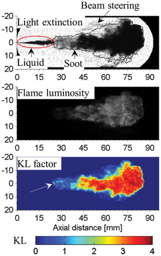
Figure 4. The saturation of detectable KL factor and measured KL factor along the radial direction at 54 mm above the nozzle tip in the light extinction image shown in Figure 3. The boundary of the natural flame luminosity is determined from the flame luminosity image in Figure 3.

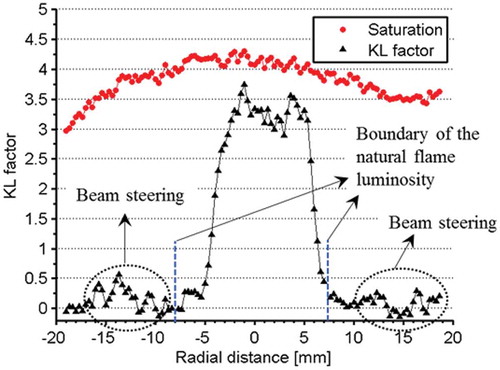
The bottom image in Figure 3 shows the final processed KL image derived from the light extinction and flame luminosity images. This image does not show the liquid jet visible in the light extinction image. However, there was a small isolated region with a high KL factor in the final processed image, whose location is indicated by a white arrow. This region is unlikely contributed by soot particles only, and is likely due to the light extinction by liquid droplets, soot and PAHs. Additionally, this small isolated spot was only observed when using nozzle N19 with a gas density of 26 kg/m³ and an injection pressure of 800 bar. The lowest pixel value in the light extinction images, which with uncertainty could be detected above the noise level, was a value of 3 of a maximum value of 255. The actual light intensity in the background images was however kept lower to avoid saturation, and varied over the images. The detectable range of KL factor values in the laser extinction setup are shown by the red dots in Figure 4, and it can be seen that it was not possible to accurately measure KL factor values larger than 4.

3.3. Soot volume fraction measurement

Two-dimensional laser extinction is a line-of-sight technique, and the data plotted in a KL factor image can be regarded as integrated values along a narrow light beam passing through the reacting jet. The measured KL factor value is the integral of the spatially local-dimensional extinction coefficient . The in the reacting jet can be calculated using the three-point Abel inversion method (Dasch, 1992), assuming cylindrically symmetry in the images of averaged diesel fuel jets, as stated above. 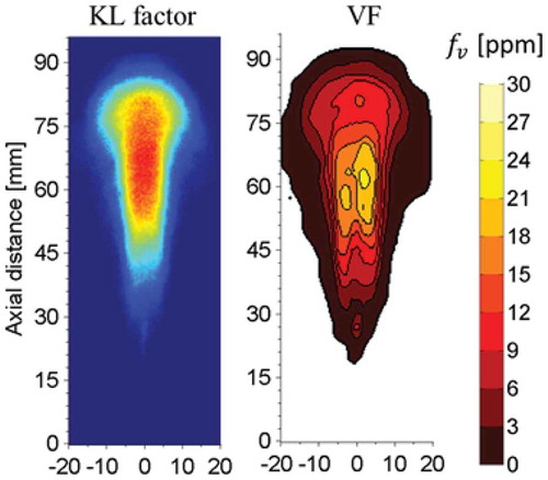Known the , the local soot VF was calculated using Equation (2). The KL factor image shown in Figure 5 represents an average over 30 injections at the same injection timing. The three-point Abel inversion was performed over the left and right halves (separated by the jet axis) of the averaged KL factor image in Figure 5. Abel inversion is very sensitive to the gradient of the KL factor, so a median filter with a 9 × 9 matrix was implemented to reduce the steep gradient of the soot VF in the center of the jet; the resulting soot VF image is shown in Figure 5. A similar procedure was implemented for the averaged OH* CL images, and the spatial distribution of OH radicals was predicted as described by Maes et al. (2016). Note that the measured soot VF and OH radical distribution obtained through the Abel inversion were all based on the averaged images. They are only to represent the average pictures of reacting diesel fuel jets rather than instantaneous ones. In addition, the predicted local equivalence ratio, which will be described in the following section, is also to represent the average picture of local equivalence ratio distribution in diesel fuel jets.

Figure 5. Averaged KL factor image and soot volume fraction (VF). The color scale for the KL factor image and experimental conditions are the same as shown in Figure 3.

3.4. Predicting the local equivalence ratio in the lift-off length region

Soot formation is strongly affected by the equivalence ratio at the lift-off length (Pickett and Siebers, 2002, 2004). To better understand the effect of the operating conditions on soot formation, the equivalence ratio was predicted using Musculus and Kattke’s variable mixture profile model (Musculus and Kattke, 2009), which is briefly described in Appendix A. The applicability of this model to non-reacting diesel jets was demonstrated by Pickett et al. (2011). However, Garcia-Oliver et al. (2017) recently reported that the air entrainment at the lift-off length region of a reacting diesel jet is around 25% lower than that in a non-reacting jet because of combustion-induced heat release. Therefore, this reduced air entrainment was taken into account for the variable mixture profile model, as described below.

Pickett et al. (2011) suggested that the best way to predict mixing and the spreading angle using the variable profile model is to couple it with measured penetration data. In our case, the penetration length (the longest axial distance from the nozzle tip) of reacting jets was determined by analyzing OH* CL images. We have previously observed (Du et al., 2017) that the penetration length determined from OH* CL images is identical to that determined from flame luminosity images when the sooting zone occupies the whole reacting jet. The same trend was also observed in this study. In addition, Desantes et al. (2014) showed that the penetration observed in flame luminosity images coincided with that in schlieren shadowgraph images (which delineate the jet’s boundary). Another reason for using OH* CL images is that they allow the jet penetration to be measured even under low or non-sooting conditions. Figure 6 shows the boundaries determined from simultaneously recorded OH* CL (black line) and flame luminosity (green line) images, overlaid on the corresponding light extinction image acquired during the expansion of the sooting zone in a reacting jet. It should be noted that the sooting zone does not occupy the whole reacting zone during the expansion of the sooting zone. When the high-temperature reaction occurs in the jet, the effect of beam steering by gas density gradient becomes apparent in the light extinction image, producing a clear signal outside the green boundary line (which indicates the position of the sooting region boundary determined by analyzing a simultaneously acquired flame luminosity image). Interestingly, the boundary determined from the OH* CL image overlaps well with beam steering effect boundary in the light extinction image.

Figure 6. The boundary of OH^* CL (black line) and the boundary of flame luminosity (green line) are overlaid on the light extinction image shown on the left. Right side: OH^* CL image. Time at 2.07 ms ASOI, the experimental conditions are the same as shown in Figure 3.

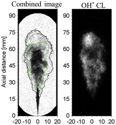
Figure 7. Measured (filled symbols) and predicted (hollow symbols) penetration lengths based on a spreading angle of 23.1°, during the steady combustion period for the N19 nozzle at an ambient gas density of 26 kg/m^3.

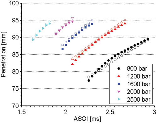
Figure 8. Soot volume fraction and OH distribution at different injection pressures for a gas density of 26 kg/m³. The left- and right-hand images in each pair show the soot volume fraction (VF) and OH distribution (OH) overlaid with the sooting zone boundary (green line), respectively. The soot volume fraction color scale is identical to that in Figure 5. Nozzle N19.

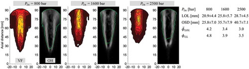
Figure 9. Soot volume fraction and OH distribution at different injection pressures under gas density 20 kg/m³. Nozzle N19.

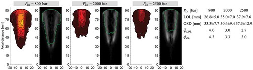
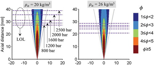
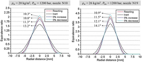
Figure 10. Predicted values of the equivalence ratio ϕ in the lift-off length (LOL) region for nozzle N19. The input spreading angles used for gas densities of 20 kg/m³ and 26 kg/m³ are 22.7° and 23.1°, respectively. The dotted line shows the edge of input spreading angle. The horizontal lines represent the averaged lift-off lengths at the different fuel pressures, and the order of the lift-off lengths with respect to the injection pressure for the 26 kg/m³ gas density is identical to that for the 20 kg/m³ density.

In Musculus and Kattke’s variable mixture profile model, the spreading angle is directly related to the air entrainment in that a larger spreading angle is associated with more air entrainment. If one used the penetration measured from the reacting jet to estimate the spreading angle for a non-reacting jet formed under the same conditions, the model would underestimate the non-reacting jet’s spreading angle and air entrainment. Desantes et al. (2014) observed that a reacting jet’s penetration length was about 10% longer than that of a non-reacting jet under the same operating conditions during the quasi-steady combustion phase. In our case, an increase of around 10% in penetration length reduced the spreading angle (and hence the air entrainment) by around 22%. Ultimately, the spreading angle was predicted from the penetration of the reacting jet, and the approximately 25% reduction of the air entrainment in the jets at the lift-off length was compensated for. It should be noted that the air entrainment upstream of the lift-off length is around 10% lower than that for a non-reacting jet (García-Oliver et al., 2017). Therefore, the reduced air entrainment upstream of the lift-off length was predicted using the spreading angle derived from the reacting penetration. This should not affect the interpretation of the predicted equivalence ratio in the lift-off region. In addition, since a smaller spreading angle was predicted for the reacting jet, the “real” spreading angle for the reacting jet should be larger than the predicted value. Regarding the predicted equivalence ratio at the lift-off length using different input spray angles, a detailed description is given in Appendix C.

Figure 7 compares the measured and predicted penetrations based on a spreading angle of 23.1° in a fully developed jet for nozzle N19 at an ambient gas density of 26 kg/m³. The measured penetrations are averaged over 30 injections and based on OH* CL images. The predicted penetrations for all injection pressures >800 bar are very close to the measured values, and the biggest difference between the predicted and measured penetration is <1.5 mm for all injection pressures. The deviation between the assumed spreading angle of 23.1° and the predicted “exact” spreading angle based on the measured penetration is <5% for all injection pressures. While the results presented in Figure 7 relate to a specific nozzle and ambient gas density, these conclusions hold for other operating conditions and the N10 nozzle.

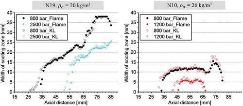
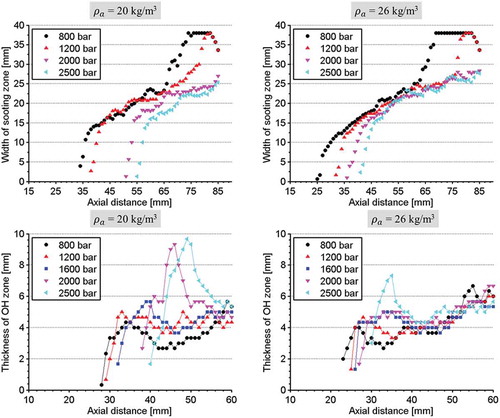
Figure 11. Sooting zone width (top) and OH zone thickness (bottom) for the N19 nozzle. The curves in the OH zone thickness graphs are cubic spline fits to the measured values.

4. Results and discussions

The optical diagnostic method developed in our previous work (Du et al., 2017) allowed us to capture time-resolved light extinction and OH* CL images. However, the results shown in the following section relate to the steady diffusion combustion phase, at 3.7 ms after start of injection (ASOI). During this period, the lift-off length was stable and the reacting jet was fully developed. Therefore, any differences between the observations relate to differences in operating conditions such as the injection pressure, gas density, and nozzle orifice diameter.

4.1. VF, OH, and ϕ in the lift-off length region for nozzle N19

Figure 8 shows the soot VF and OH distribution at different injection pressures for nozzle N19 at a gas density of 26 kg/m³. The left-hand images in each pair show the soot VF, and the right-hand images show the OH distribution overlaid with sooting zone, defined as the boundary from the corresponding averaged flame luminosity image. Similar image pairs will be shown in Figures 9 and 13. As seen in Figure 8, the boundary of the soot VF is larger than the boundary of the sooting zone in the “OH” image. This is because the boundary of sooting zone (green lines) in the “OH” images was determined by selecting a threshold value of 1% on the averaged flame luminosity images. However, the soot VFs images are obtained from the averages of individual KL images, with borders determined in each individual image.

Figure 12. Probability of sooting throughout the reacting jet. The color scale for the images is shown on the far right; a value of “1” indicates 100% probability of soot formation in all cases.

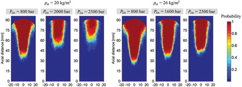
Figure 13. Soot volume fractions and OH distributions at different injection pressures for gas densities of 20 kg/m³ (top) and 26 kg/m³ (bottom) using nozzle N10. The image pairs on the left of the figure and in the center show the soot volume fraction (VF; leftmost image of the pair) and OH distribution (OH; rightmost image of the pair) with a green line denoting the boundary of the sooting zone. The color scale for the soot volume fraction images is shown on the far left. The white arrows shown at injection pressure of 1600 bar indicate the zones without OH radicals.

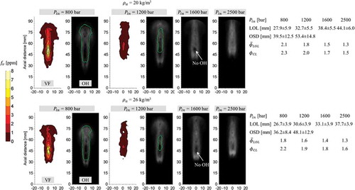
In Figure 8, “LOL” indicates the lift-off length (see description of measurement in Appendix B), “OSD” indicates the onset of soot formation axial distance from the nozzle tip, is the predicted averaged cross-sectional equivalence ratio at the lift-off length, and is the predicted equivalence ratio along the jet’s center line at the lift-off length. The method used to predict is described in Appendix B, and the prediction of is based on the predicted variable mixture profile. Two standard deviations for the measured LOL and OSD over 30 injection events are also given, and the same symbols and abbreviations are used in Figures 9 and 13.

Figures 8 and 9 show that as the injection pressure increases, the area of maximum soot VF in the “VF” images decreases and the axial distance interval between the LOL and OSD increases. In addition, there is a zone with no OH radicals in the center of the “OH” images, with the OH radicals being concentrated in the periphery of the jet. Such computed OH distribution structures are expected to be enhanced by a combination of OH* signal trapping and soot incandescence in the jet center, and the long integral length of OH* chemiluminescence in the jet edge. The OH distribution structure observed in this study is consistent with the findings of Maes et al. (2016) and the conceptual diesel spray flame model presented by Kosaka et al. (2005). As shown in Figure 9, when using nozzle N19 with an injection pressure of 2500 bar, reducing the gas density to 20 kg/m³ significantly reduced the soot VF.

One factor responsible for the reduced maximum soot VF area is the reduction of the local equivalence ratio in the lift-off region in response to increases in the injection pressure or reductions in gas density. This is consistent with the observations of Pickett and Siebers (2004), who found that the averaged integral soot VF decreased when was reduced by raising the injection pressure or reducing the gas density. Figure 10 shows the predicted equivalence ratio in the lift-off length region for nozzle N19 at the 20 kg/m³ and 26 kg/m³ gas densities. It should be noted that the decreases as the axial distance increases. In addition, the rates of air entrainment and fuel injection are both proportional to the injection pressure. Therefore, the local equivalence ratio within the jet is expected to be independent of the injection pressure; and the same equivalence ratio profile was used for the different injection pressures. As shown in Figure 10, the lift-off length region where the high-temperature reaction occurs is shifted further downstream in the jet as the injection pressure increases, i.e., higher injection pressures yield longer lift-off lengths. This reduces the local in the lift-off length region at both gas densities. Studies on laminar premixed flames (Arana et al., 2004; Melton et al., 2000) showed that the equivalence ratio strongly influences the formation of PAHs and soot. In a lifted reacting diesel diffusion jet, the fuel and air are partially premixed upstream of the lift-off region. Therefore, trends observed in premixed flames should also be observed in lifted reacting diesel jets. In addition, Kent and Honnery (1987) found that the reduction in the soot VF in turbulent diffusion flames correlated well with reductions in the predicted mixture fraction.

Although the predicted local profile increases when the gas density is reduced from 26 kg/m³ to 20 kg/m³, the longer lift-off lengths seen at the lower density cause the local in the lift-off length region to be lower at any given injection pressure. Consequently, the soot VF is lower at the lower gas density.

Another factor is the effect of the residence time on soot formation. Early studies on turbulent diffusion flames (Kent and Honnery, 1987; Kent and Wagner, 1984) indicated that the soot VF depended on the residence time nearer the nozzle in the early soot formation region (when the residence time is short). Lee et al. (2009) also found that the onset of soot formation began increasingly far downstream of the nozzle as the jet velocity increased because the residence time near the nozzle decreased.

Interestingly, Figure 8 also shows that the maximum soot VF range was independent of the injection pressure at the 26 kg/m³ gas density. The absolute soot VF measurement is difficult at high soot concentration conditions (e.g., when the KL factor is higher or near 4.0). In our measurement, the light extinction images were captured at similar laser power and the KL factor in all averaged images are lower than 4.0. Therefore, it is assumed that the measured maximum soot VF shows the qualitative trend. As shown in Figure 9, the tendency for the maximum soot VF to decrease as the jet velocity increased was observed under low gas density conditions (20 kg/m³). The difference in the behaviors observed at low and high gas densities may be because of the high > 3.5) observed at the high gas density. Such high equivalence ratios strongly favor soot formation. This is also probably related to the thickness of the OH zone along the axial length of the jet. The following section discusses these issues in more detail.

At all tested injection pressures, raising the gas density from 20 to 26 kg/m³ also reduced the distance interval between the LOL and OSD (see Figures 8 and 9). This observation is consistent with observations of laminar flames at elevated ambient pressures (Thomson et al., 2005; Tsurikov et al., 2005), in which the onset of soot formation distance was shifted closer to the nozzle when the ambient pressure (which corresponds to the gas density in this work) was increased. Therefore, increasing the ambient pressure promoted soot formation (Thomson et al., 2005). In addition, Tsurikov et al. (2005) showed that the OSD was shifted closer to the nozzle at any given ambient pressure when the equivalence ratio increased. This implies that in addition to the residence time, the OSD varies with the equivalence ratio and ambient pressure.

4.2. Sooting zone width, OH zone thickness, and probability of soot formation for nozzle N19

As stated in the “Introduction,” reduced soot formation in the radial direction of a reacting jet was observed in our previous study (Du et al., 2017). This section explores the possibility of a correlation between the reduced soot formation in the radial direction and an increase in the thickness of the OH zone. Figure 11 shows the measured sooting zone width (or equivalently, the radial soot path length) and the OH zone thickness for the nozzle N19 at gas densities of 20 and 26 kg/m³. The sooting zone width was determined by analyzing averaged flame luminosity images, and the threshold for defining the boundary was set at 1% of the maximum pixel value (255). Since the natural flame luminescence intensity in diesel flames depends on the soot temperature, there will some uncertainty in the sooting zone widths determined by the flame luminosity images. However, in our measurements, it was found that the sooting zone widths determined from the flame luminosity images closely coincided with the ones determined from the KL factor images with a threshold value of 0.03, see detailed discussions in Appendix D. The thickness of the OH zone was measured using the right-half parts of “OH” images presented in Figures 8 and 9, using a threshold of 15% of the maximum pixel value (255). This procedure was also used to generate the results shown in Figure 15.

Figure 14. Predicted the equivalence ratio ϕ in the lift-off length (LOL) region for the nozzle N10. The input spreading angle for the gas density 20 kg/m³ and 26 kg/m³ are 21.6° and 20.8°, respectively. The dotted line is the edge of input spreading angle. The horizontal lines represent the averaged lift-off lengths at the different fuel pressures. For the gas density 26 kg/m³, the shown lift-off length from the upstream to the downstream of axial distance is the same as the order shown for gas density 20 kg/m³. The scale of color bar is shown in the far right.

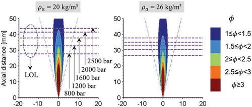
Figure 15. Sooting zone width (top) and OH zone thickness (bottom) for nozzle N10. The curves on the OH zone thickness graphs are cubic spline fits to the data.

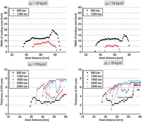
As can be seen in Figure 11, the width of the sooting zone increases significantly at axial distances >60 mm when the injection pressure is 800 or 1200 bar. This is due to vortices in the jet head, which also affect the OH radical distribution. These vortices are not observed when the injection pressure is >1200 bar, because the jet head has already developed too far downstream. To avoid the complications this creates, the thickness of the OH zone is only reported for axial distances up to 60 mm. As shown in Figure 11, injection pressures of 1200–2500 bar yield very similar sooting zone widths at axial distances >50 mm when the gas density is 26 kg/m³. This is consistent with Pickett and Siebers’ findings (2004). However, this is not the case for axial distances <50 mm, where the OH zone thickness increases slightly with the injection pressure. At a gas density of 20 kg/m³, the reduction in sooting zone width clearly correlates with the increase in OH zone thickness as the injection pressure rises. This is consistent with the important role of OH radicals in soot oxidation: an increase in the abundance of OH radicals would be expected to suppress soot growth (Lee et al., 2009). In addition to the slight reduction in sooting zone width at higher injection pressures, the maximum soot VF decreases significantly (as shown in Figure 9). Neither of these trends was observed with a gas density of 26 kg/m³, which was attributed to the very high soot formation rate (>3.5) observed for all injection pressures under the high density conditions (see Figure 8); the increase in OH radical zone width at higher injection pressures was apparently not sufficient to counterbalance this effect. This may explain Pickett and Siebers’ finding (2004) that the optical path length (i.e., the sooting zone width) was independent of the injection pressure.

The probability of sooting across the entire jet was calculated from the flame luminosity images over 30 injections and is shown in Figure 12. At a gas density of 26 kg/m³, the zone corresponding to a sooting probability of 100% occupies almost the entire sooting region at all injection pressures. At a gas density of 20 kg/m³, the maximum sooting probability region gradually shrinks in the radial and axial directions as the injection pressure increases. This observation is consistent with the discussion above, supporting the hypothesis that there is a correlation between the sooting zone width, OH zone thickness, the value at the lift-off length, and the maximum soot VF.

4.3. VF, OH, and ϕ at the lift-off length region for nozzle N10

Figure 13 shows the soot VF and OH distribution for nozzle N10. Soot VF images are only shown for injection pressures of 800 and 1200 bar. When the injection pressure was >1200 bar, no flame luminosity was detectable. Therefore, only OH distribution images are shown for injection pressures of 1600 and 2500 bar. Additionally, the measured OSD value shown for the 1200 bar injection pressure in Figure 13 was averaged over results for sooting jets only.

At injection pressures of 800 and 1200 bar, the OH distributions at gas densities of 20 and 26 kg/m³ were similar to those shown in Figures 8 and 9, which feature a no OH radical zone (shown in black) in the center of the “OH” images, with OH radicals being localized in the periphery of the jet. However, as shown in Figure 13, these non-OH radical zones were much smaller when using nozzle N10, and do not occupy the entire center area unlike those shown in Figures 8 and 9, which present results obtained with nozzle N19. This is mainly due to the much lower equivalence ratio at the lift-off region with nozzle N10 compared to nozzle N19. Consequently, with nozzle N10, the region of available OH radicals expands toward in the jet center, and they oxidize the fuel mixture more completely and much less soot is produced. It should be noted that the soot VFs signified by specific colors in the color scale for Figure 13 are 3.75 times lower than those for the color scale used in Figures 8 and 9. The use of nozzle N10 also causes an upstream shift of the axial distance at which the maximum soot VF begins relative to that for nozzle N19, as can be seen by comparing Figure 13 to Figures 8 and 9. This implies that the axial position of the maximum soot VF depends on the nozzle outlet diameter. The use of the N10 nozzle also causes OH radicals to be observed further downstream in the jet (i.e., in the jet head) at injection pressures of 800 and 1200 bar. One would therefore expect soot particles formed in the upstream region to be oxidized by the OH radicals in the jet head (observable this behavior in Figure 19). As a result, the soot VF in the jet head is greatly reduced.

Figure 16. Probability of sooting across the reacting jet for nozzle N10. The color scale is shown on the far right; a value of “1” indicates 100% probability of sooting for all injection events.

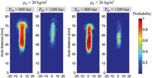
Figure 17. The maximum KL factor in the images as the function of ϕ. Experimental data were collected at the injection pressures of 800, 1200, and 1600 bar under gas densities of 20 and 26 kg/m³ for nozzle N10.

Figure 18. The lift-off length in all injection events recorded at an injection pressure of 1200 bar using nozzle N10 at 3.7 ms ASOI. The ϕ values are computed using the predicted Φ shown in Figure 12. The numbers “1, 2, 3” in the circles represent possible non-sooting states, and the number “4, 5, 6” in the circles indicate potentially sooting states. The black dashed lines show the averaged lift-off length, and the violet dashed lines show the maximum and minimum lift-off lengths.

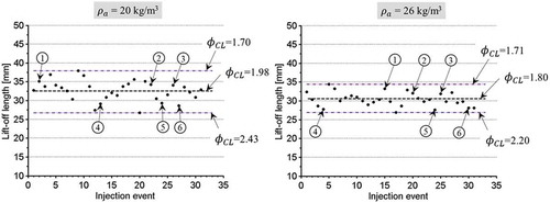
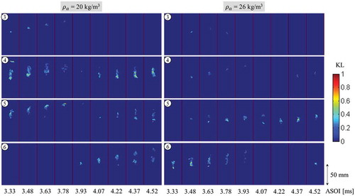
Figure 19. Instantaneous KL image series at gas densities of 20 kg/m³ (left) and 26 kg/m³ (right). The circled numbers correspond to those in Figure 18. In all images, the nozzle tip is located on the vertical center line, at the bottom of the image. The color scale for the KL images is shown on the right. The image series show results captured during the steady combustion phase, and the lift-off length is almost constant.

For the non-sooting jets formed with an injection pressure of 1600 bar at gas densities of 20 and 26 kg/m³, small zones without OH radicals are present in the jet’s upstream region. These regions are almost completely absent when the injection pressure is raised to 2500 bar. The technique used to visualize the OH radical distribution is based on Abel inversion of averaged line-of-sight OH* CL images. Unfortunately, this technique lacks spatial resolution, and it is not clear that the apparent uniform intensity seen in the OH images reflects a genuinely uniform distribution of OH radicals across the jet. If such a uniform distribution were present, the non-sooting nature of the jet would imply that the high-temperature reaction to occur across the entirety of the jet. This would yield a combustion process similar behavior that has been observed under very lean (non-sooting) combustion conditions by Taschek et al. (2005a), (2005b)). Unfortunately, the methods used in this work do not permit us to confidently state that the OH radical distribution is as entire as it appears in our images, so this result requires further investigation.

Figure 14 shows the predicted equivalence ratio in the lift-off length region for the nozzle N10 at gas densities of 20 kg/m³ and 26 kg/m³. It should be noted that the values corresponding to specific colors in the color scale for this figure are lower than those for the scale used in Figure 10. It should also be noted that the input spreading angle for the gas density of 20 kg/m³ is about 4% larger than that for the 26 kg/m³ density. This may be due to an increase in the ratio of the reacting spreading angle to the inert (non-reacting) spreading angle as the gas density decreases; a trend of this sort was observed by Desantes et al. (2014) using a nozzle orifice diameter of 0.082 mm. It was not possible to verify that the reacting spreading angle at the low gas density of 20 kg/m³ is greater than that at 26 kg/m³. However, the predicted equivalence ratio based on the predicted spreading angles used in Figure 14 gives reasonable explanations for the experimental results, as discussed below.

The predicted profile for nozzle N10 shown in Figure 14 is much less sensitive to change in the gas density than that for nozzle N19 (which is shown in Figure 10). The values for all injection pressures at a gas density of 20 kg/m³ are slightly higher than those for a density of 26 kg/m³. Therefore, as shown in Figure 13, for injection pressures of 800 and 1200 bar, the maximum soot VF at a gas density of 20 kg/m³ was consistently slightly >26 kg/m³.

The values observed with nozzle N19 (see Figure 10) are consistently around twice those seen with nozzle N10 (see Figure 14). This is consistent with the experimental observations of Bruneaux et al. (2011) in a diesel-like gas jet (i.e., a gas jet resembling a liquid diesel jet under HP/HT diesel chamber conditions). They found that reducing the nozzle hole diameter increased the air entrainment rate (the ratio of the flow rates of air and fuel) by a factor that scaled approximately with the diameter. This would explain the lower soot VF observed with nozzle N10 (see Figures 8, 9 and 13) at the 800 bar injection pressure because the value at this injection pressure is close to the well-established non-sooting limit of <2. Interestingly, the soot VF is not zero with nozzle N10 and an injection pressure of 1200 bar even though under these conditions is < 2. This is because the measured lift-off lengths are averaged over 30 injections, and the soot VF images are based on the averaged images. One factor could be that temperature fluctuations in the chamber caused fluctuations in the lift-off length because the lift-off length varies with the temperature as , as shown by Siebers and Higgins (2001). As will be seen in Figure 16, the maximum probability of sooting for the 1200 bar injection pressure is about 60% for both gas densities. The effects of lift-off length fluctuations on soot formation at the 1200 bar injection pressure are discussed more extensively in the next section.

For injection pressures of 1600 and 2500 bar, the values in radial and axial directions in the lift-off length region are well below the sooting threshold of <2. Therefore, no soot formation was observed under these conditions.

As shown in Figure 13, the distance interval between the LOL and OSD increases as the gas density decreases. A similar trend was observed with nozzle N19. This supports the conclusion that the OSD depends on the ambient pressure as well as the residence time.

4.4. Sooting zone width, OH zone thickness, and probability of soot formation for nozzle N10

The trend observed with nozzle N19 at a gas density of 20 kg/m³ was reproduced with nozzle N10: the sooting zone width decreased as the injection pressure increased (as shown in Figure 15) and the maximum soot VF decreased significantly (as shown in Figure 13). This can be correlated to the increased OH zone thickness seen in Figure 15, and the reduction in as shown in Figure 14. These factors reduce soot formation. Higher injection pressures therefore shrink the region of maximum sooting probability in the radial and axial directions, as shown in Figure 16. It should be noted that the for nozzle N10 at both gas densities is <2.3, leading to very low soot formation.

In addition, the sooting zone width at a gas density of 26 kg/m³ for injection pressures of 800 bar and 1200 bar is smaller than at 20 kg/m³. This can be correlated with the increase in the OH zone thickness at the 26 kg/m³ density, which is shown in Figure 15. It can also be correlated with decrease in at 26 kg/m³, as shown in Figure 13.

For non-sooting jets, i.e., those formed at injection pressures of 1600, 2000, and 2500 bar at both gas densities, the OH zone thickness peaks just downstream of the lift-off length. Notably, at injection pressures of 2000 and 2500 bar, the OH zone thickness becomes almost constant after reaching its maximum value. This suggests that the OH radicals are indeed distributed in the entire jet, as suggested by the images shown in Figure 13.

4.5. The effect of ϕ on the soot formation

As shown in Figure 16, the maximum probability of sooting at an injection pressure of 1200 bar is about 60%. This indicates that some injection events produce soot in the jets and other do not. To determine whether the in these non-sooting jets were below the critical non-sooting threshold (e.g., assuming < 2), the maximum KL factor in the image as the function of is shown in Figure 17. The data presented in Figure 17 is the experimental conditions at the injection pressures of 800, 1200, and 1600 bar under gas densities of 20 and 26 kg/m³, and the total amount of points is over 180 injections. The estimated is based on the measured lift-off lengths for each individual injection event recorded (at 3.7 ms ASOI) under these conditions, because the lift-off length fluctuates at each condition, leading to variations in . For comparative purposes, we assume that changes in the lift-off length do not change the predicted profile in Figure 14, and the other experimental conditions are the same. Therefore, any differences in the maximum KL factor can be correlated with changes in the local in the lift-off length region. The range of in Figure 17 covers 1.5 to 2.8, so that effect of on the soot formation is examined in a statistic way.

The probability of non-sooting at <2 is calculated as the amount of non-sooting (i.e., KL factor 0) points at <2 divided by the total points at <2, and the same procedure is applied for other non-sooting and sooting cases. As shown in Figure 17, the probability of non-sooting at <2 is about 80%, and it increases when the critical threshold decreases to 1.9. A similar trend was also observed for the probability of sooting. The probability of non-sooting/sooting is about 80% when the threshold of for non-sooting/sooting is set at 2.0 ± 0.1. This trend implies that has a critical effect on soot formation and the rate of soot formation. In addition, the predicted ϕ profile shown in Figure 14 is appropriate based on the method applied in this paper because the probability of non-sooting/sooting can be reasonably explained using the predicted value.

To further interpret the effect of on the soot development, the measured lift-off lengths for each individual injection event recorded (at 3.7 ms ASOI) at the injection pressure of 1200 bar are plotted in Figure 18. Injection events corresponding to non-sooting and sooting conditions are selected. The arrows labeled 1, 2, and 3 indicate representative data points corresponding to the non-sooting conditions. No detectable KL was observed during the injection events corresponding to points 1 and 2, and only a small KL spot was seen during injection event 3. The arrows labeled 4, 5, and 6 indicate representative data points with elevated values, corresponding to sooting conditions. As shown in Figure 19, the KL images of these injection events clearly show detectable KL areas. The KL image series recorded under low sooting conditions such as those during injection events 4, 5, and 6 (see Figure 19) exhibit only intermittently detectable KL levels. This is consistent with results obtained for turbulent diffusion flames (Lee et al., 2009; Lignell et al., 2007), which exhibit very large spatial and temporal variation in the extent of their soot fields. The figure also clearly shows that the KL (soot concentration) area is much smaller than the OH area shown in Figure 13. This supports the conclusion that levels of soot particles are reduced in both the radial and axial directions.

In this paper, soot formation was correlated to rather than . This should not be taken to imply that is more generally useful than for explaining trends in soot formation. In fact, as shown in Figures 8, 9 and 13, the soot formation trends observed in this work can also reasonably be explained in terms of . Moreover, the values observed in this work were generally around 10–20% greater than the corresponding , which is consistent with previously reported ratios (Pickett et al., 2011). Using would provide another option for interpreting observed trends in soot formation. Furthermore, Musculus and Kattke’s variable mixture profile makes it possible to predict the local equivalence ratio in the lift-off length region. In this study, the probability of non-sooting was over 80% when the threshold of was set as 2.0. However, the exact threshold value has not been validated. Since the threshold value used in this paper indicated the soot formation trend reasonably, it can be assumed that when the is less than the critical threshold 2.0, the non-sooting conditions likely occur, at least it satisfies our operating conditions.

5. Conclusions

This paper presents the results of studies on soot formation and oxidation in reacting diesel jets conducted using an optically accessible HP/HT rig. Two-dimensional light extinction, flame luminosity, and OH* CL images were captured at a constant ambient temperature of 823 K and two gas densities (20 and 26 kg/m³), at injection pressures of 800–2500 bar using nozzle orifices with diameters of 0.19 and 0.10 mm. Soot VF and OH distribution images were obtained using the three-point Abel inversion method, and the local equivalence ratio in the lift-off length region was predicted using Musculus and Kattke’s variable mixture profile model.

The major conclusions of this study are as follows:

• Predicted local equivalence ratios based on penetration lengths determined by analyzing OH* CL images provided reasonable explanations for the observed trends in soot formation. was found to have a critical effect on soot formation and when the was >2.0 soot was likely formed in the jet. Soot was unlikely formed when the was lower than 2.0. Further reductions in yielded completely non-sooting conditions.

• Reductions in increased the OH zone thickness in the jet’s upstream region, reducing the area of maximum soot VF. The increase in the OH zone thickness correlated well with reductions in the sooting zone width. However, under high sooting conditions (e.g., >3.5), the sooting zone width in the downstream region was independent of .

• For non-sooting jets, the OH zone thickness peaked just downstream of the lift-off length. For low values (around 1.5), the OH zone thickness rose to a maximum and then remained near-constant.

• The distance interval between the LOL and OSD increased when the injection pressure increased, or the ambient pressure decreased, or the local equivalence ratio fell.

• The location of maximum soot VF in the jet depended on the nozzle orifice diameter, and was closer to the nozzle tip for nozzle N10 than for nozzle N19.

Acknowledgments

The authors thank Scania CV AB who provided fuel injection system. The assistance of research engineers at the combustion division is also gratefully acknowledged.

Additional information

Funding

This work was supported by the CERC (Combustion Engine Research Centre at Chalmers).

Appendix A.

Musculus and Kattke’s variable mixture profile

Figure A1 depicts the Musculus and Kattke’s variable mixture profile model and its key variables. The mass radial profiles are given as follows:

(A-1)

Figure A1. Illustration of the one-dimensional transient diesel jet model of Musculus and Kattke (2009).

where is the turbulent mean volume fraction, the subscript denotes the values on the jet centerline, is the ratio of the radial coordinate to the jet width , and is the full spreading angle. For a fully developed shape some distance downstream of the jet, the exponent 1.5. The mass distribution profile has the same radial velocity profile as shown in Figure A1, and resembles a Gaussian function.

An important input for this model is the spreading angle of the diesel jet. In our case, based on the measured penetration length from the OH* CL images, the input spreading angle for the variable mixture profile model was estimated using the following equation:

(A-2)

where , is the non-dimensional axial penetration distance, is the non-dimensional penetration time, and = 105/52 is constant for a fully developed jet. The non-dimensional axial penetration distance is , where , , and is the axial distance from the nozzle tip to the maximum length of jet. is a characteristic length scale for the fuel jet. The characteristic length scale is defined as

(A-3)

In our case, is the measured penetration length from OH* CL images. The non-dimensional penetration time is , where the characteristic time scale () for penetration is defined as

(A-4)

where is the cross-sectionally average velocity at the nozzle exit. For the variable mixture profile, the parameters and in Equations (A3) and (A4) were set to one. The penetration predicted by Pickett et al. (2011) using the simplified Equation (A2) was almost identical to the exact solution, deviating by <0.5 mm.

Appendix B.

The estimation of ϕ

Lift-off lengths were determined by analyzing individual OH* CL images using a method similar to that described by Higgins and Siebers (2001), using a threshold of 5% of the maximum OH* CL image pixel value (255). The averaged cross-sectional equivalence ratio at the lift-off length, , was estimated using an expression developed by Pickett and Siebers (2004):

(B-1)

where is the stoichiometric air-fuel ratio by mass and is a characteristic length scale for the fuel jet. The characteristic length scale is defined as

(B-2)

where is the injected fuel density, is the air density, is the area contraction coefficient of the nozzle orifice, and is the orifice outlet diameter. A value of 0.75 was initially suggested for the constant a (Pickett and Siebers, 2004; Siebers et al., 2002), but it was later suggested by Pickett et al. (2011) that a value of < 0.70 might yield a better match to the variable-profile penetration in the downstream region of the jet. Therefore, the constant a was set to 0.68. The input spreading angle for Equation (B2) was estimated using the empirical equation developed by Siebers (1999):

(B-3)

where the coefficient B only depends on the orifice outlet diameter. Note that the input spreading angle estimated using Equation (B3) is only used in Equation (B2), and not in Musculus and Kattke’s variable mixture profile model.

Appendix C.

The estimation of local equivalence ratio depending on the spray angle

Musculus and Kattke’s model is developed for an inert jet. However, because of the reduction of air entrainment due to the heat release at the lift-off length region, the reduction of air entrainment should be taken into account when using the Musculus and Kattke’s model to predict the equivalence ratio at the lift-length region. In this work, a reduction of air entrainment was taken into account at the lift-off length region in the Musculus and Kattke’s variable mixture profile. That is to use the reacting penetration length to compensate approximately 25% reduction in predicted air entrainment along the jet’s center at the lift-off length, because the penetration of the reacting jet is about 10% longer than that of the non-reacting jet. Figure C1 shows the predicted equivalence ratio profiles at the lift-off length using different input spray angles. The equivalence ratio predicted using the spray angle estimated by the reacting penetration is shown as the red dash line as “Reacting.” If assuming that the inert penetration is 10% shorter than the reacting one, then the input spray angle increases about 22% compared to the input spray angle using the reacting jet. The corresponding predicted equivalence ratio at the jet’s center in the lift-off length decreases about 25%, i.e., about 25% more air is entrained. This is shown as “Inert” one in Figure C1. The predicted equivalence ratios using 5% decrease/increase in the input spray angle of the reacting jet are also shown in Figure C1. As can be seen that 5% decrease/increase in the input spray angle increases/decreases the predicted about 5%, and the relationship between the input spray angle and the predicted is almost linear. As shown clearly in Figure C1, the predicted using the input spray angle for the reacting penetration is about 25% higher than the one using the input spray angle of the inert one for both cases. Although two specific conditions are shown in Figure C1, this trend can also extend to other operating conditions in this work. In addition, it also can be seen that the predicted equivalence ratio using the reacting jet is lower in the jet edge region (from −7.5 mm to −2.5 mm and from 2.5 mm to 7.5 mm) than the one using the inert jet. This does not stand for the physical sense. However, this would not influence the predicted in this work.

Figure C1. Comparison of predicted equivalence ratio at the lift-off length using different input spray angles. The lift-off lengths in the corresponding conditions can be referred in Figures 10 and 14. The half of spreading angles () at the corresponding conditions are also shown.

Appendix D.

The measurement of sooting zone widths

Pickett and Siebers (2004) showed that the spatial locations of soot in the planar laser induced incandescence images closely coincided with the ones captured by the natural flame luminosity images, suggesting that the natural flame luminosity in reacting diesel sprays is primarily due to the hot soot particles. Therefore, analyzing the flame luminosity images could provide a possibility to determine the sooting zone widths. Because the natural flame luminosity in a diesel spray flame is due primarily to natural incandescence from hot soot, the intensity of the flame luminosity depends on both the soot abundance and the soot temperature. To determine the radial soot path lengths (corresponding to the width of sooting zone in this report) at various experimental conditions, Pickett and Siebers (2004) selected 5% of the peak flame luminosity at the laser extinction measurement height as the threshold to determine the soot path lengths. To examine the sooting zone widths determined from the averaged flame luminosity images in our measurement, the KL factor and flame luminosity as function of the radial direction at 60 mm above the nozzle tip are shown in Figure D1. The overall intensity distribution in the two images is different, with a maximum in KL factor along the center axis, whereas there is a small dip in the center in the flame luminosity. One reason for the dip is that the flame temperature, and thereby the soot particle temperature, is lower in the center where the equivalence ratio is high, compared to the edges where the conditions are closer to stoichiometric. Another reason is signal attenuation, i.e., the luminescence light emitted by soot particles far from the camera, will be attenuated by absorption by other soot particles along the way toward the camera. The higher the KL factor, the stronger the signal attenuation effect, but close to the edges the KL factor is low and the effect on the detected luminescence signal is small. As can be seen in Figure D1, the sooting zone width determined from the averaged flame luminosity image with a threshold value 1% of the maximum pixel value (255) is close to the one determined from the averaged KL factor image with a threshold value of 0.03. Figure D2 shows the sooting zone widths determined from averaged flame luminosity (with filled color) and averaged KL factor (hollow symbols) images, and the threshold values were 1% of the maximum pixel value (255) and 0.03 for the flame luminosity and KL factor image, respectively. As can be seen in Figure D2, the sooting zone widths determined from both images closely coincide under different experimental conditions. This relationship was found to be true for other conditions as well. Therefore, in this work, the sooting zone widths were determined by the flame luminosity images, and the threshold for defining the boundary was set at 1% of the maximum pixel value (255). Pickett and Siebers (2004) also observed that the radial soot path lengths were not affected by changes in ambient temperature or injection pressure. However, the soot path lengths were significantly affected by the ambient gas density. Hence, comparisons of the sooting zone widths in this work were only made between different injection pressures at other fixed experimental conditions. Due to the beam steering effects on the jet edges in the light extinction images in our measurements, the determination of sooting zone width solely from the KL factor images was difficult, in particular, for the low sooting conditions. This is another reason for choosing the flame luminosity images to determine the sooting zone widths. Note that there is uncertainty in the measured absolute sooting zone widths using the flame luminosity images. However, the observed experimental trends which were affected by the injection pressure in the sooting zone widths would not be affected.

Figure D1. KL factor and flame luminosity as function of the radial direction at 60 mm above the nozzle tip (right graph). The gray dashed lines in averaged KL factor (left) and flame luminosity (middle) images indicate the selected 60 mm above the nozzle tip. The color scale for the KL factor image is the same as shown in Figure 3. The blue and green lines in KL factor and flame luminosity graph (right) are the determined boundaries of the sooting zone in KL and flame luminosity images, respectively. The corresponding threshold values are shown. The curves on the KL factor and flame luminosity are cubic spline fits to the data. Experimental conditions: injection pressure 800 bar, gas density 20 kg/m³, 3.7 ms AOSI, nozzle N19.

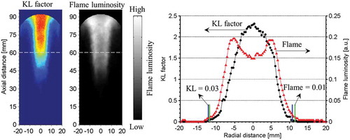
Figure D2. Determined sooting zone widths from the averaged flame luminosity (filled symbols) and averaged KL factor (hollow symbols) images at different experimental conditions. Threshold values are 1% of the maximum pixel value (255) and 0.03 for the flame luminosity and KL factor images, respectively.

References

- Arana, C., Pontoni, M., Sen, S., and Puri, I. 2004. Field measurements of soot volume fractions in laminar partially premixed coflow ethylene/air flames. Combust. Flame, 138, 362–372.
- Bruneaux, G., Causse, M., and Omrane, A. 2011. Air entrainment in diesel-like gas jet by simultaneous flow velocity and fuel concentration measurements, comparison of free and wall impinging jet configurations. SAE Int. J. Engines, 5, 76–93.
- Choi, M., Mulholland, G., Hamins, A., and Kashiwagi, T. 1995. Comparisons of the soot volume fraction using gravimetric and light extinction techniques. Combust. Flame, 102, 161–169.
- Dasch, C. 1992. One-dimensional tomography: a comparison of Abel, onion-peeling, and filtered backprojection methods. Appl. Opt., 31, 1146.
- Desantes, J., Pastor, J., García-Oliver, J., and Briceño, F. 2014. An experimental analysis on the evolution of the transient tip penetration in reacting Diesel sprays. Combust. Flame, 161, 2137–2150.
- Du, C., Andersson, M., and Andersson, S. 2016. Effects of nozzle geometry on the characteristics of an evaporating diesel spray. SAE Int. J. Fuels Lubr., 9, 493–513.
- Du, C., Andersson, S., and Andersson, M. 2017. Soot formation and oxidation in a turbulent diffusion diesel flame: the effect of injection pressure. Submitted to the publication.
- García-Oliver, J., Malbec, L., Toda, H., and Bruneaux, G. 2017. A study on the interaction between local flow and flame structure for mixing-controlled diesel sprays. Combust. Flame, 179, 157–171.
- Higgins, B., and Siebers, D. 2001. Measurement of the flame lift-off location on DI diesel sprays using OH chemiluminescence. SAE 2001-01-0918.
- Kent, J., and Honnery, D. 1987. Soot and mixture fraction in turbulent diffusion flames. Combust. Sci. Technol, 54, 383–398.
- Kent, J., and Wagner, H. 1984. Why do diffusion flames emit smoke. Combust. Sci. Technol., 41, 245–269.
- Kosaka, H., Aizawa, T., and Kamimoto, T. 2005. Two-dimensional imaging of ignition and soot formation processes in a diesel flame. Int. J. Engine Res., 6, 21–42.
- Krishnan, S., Lin, K., and Faeth, G. 2000. Optical properties in the visible of overfire soot in large buoyant turbulent diffusion flames. J. Heat Transfer, 122, 517–524.
- Lee, S., Turns, S., and Santoro, R. 2009. Measurements of soot, OH, and PAH concentrations in turbulent ethylene/air jet flames. Combust. Flame, 156, 2264–2275.
- Lignell, D., Chen, J., Smith, P., Lu, T., and Law, C. 2007. The effect of flame structure on soot formation and transport in turbulent nonpremixed flames using direct numerical simulation. Combust. Flame, 151, 2–28.
- Maes, N., Meijer, M., Dam, N., Somers, B., Baya Toda, H., Bruneaux, G., Skeen, S., Pickett, L., and Manin, J. 2016. Characterization of Spray A flame structure for parametric variations in ECN constant-volume vessels using chemiluminescence and laser-induced fluorescence. Combust. Flame, 174, 138–151.
- Manin, J., Pickett, L., and Skeen, S. 2013. Two-color diffused back-illumination imaging as a diagnostic for time-resolved soot measurements in reacting sprays. SAE Int. J. Engines, 6, 1908–1921.
- Melton, T., Inal, F., and Senkan, S. 2000. The effects of equivalence ratio on the formation of polycyclic aromatic hydrocarbons and soot in premixed ethane flames. Combust. Flame, 121, 671–678.
- Migliorini, F., Thomson, K., and Smallwood, G. 2011. Investigation of optical properties of aging soot. Appl. Phys. B, 104, 273–283.
- Musculus, M., and Kattke, K. 2009. Entrainment waves in diesel jets. SAE Int. J. Engines, 2, 1170–1193.
- Nakakita, K., Nagaoka, M., Fujikawa, T., Ohsawa, K., and Yamaguchi, S. 1990. Photographic and three dimensional numerical studies of diesel soot formation process. SAE 902081.
- Pickett, L., Manin, J., Genzale, C., Siebers, D., Musculus, M., and Idicheria, C. 2011. Relationship between diesel fuel spray vapor penetration/dispersion and local fuel mixture fraction. SAE Int. J. Engines, 4, 764–799.
- Pickett, L., and Siebers, D. 2002. An investigation of diesel soot formation processes using micro-orifices. Proc. Combust. Inst., 29, 655–662.
- Pickett, L., and Siebers, D. 2004. Soot in diesel fuel jets: effects of ambient temperature, ambient density, and injection pressure. Combust. Flame, 138, 114–135.
- Pickett, L., and Siebers, D. 2005. Orifice diameter effects on diesel fuel jet flame structure. J. Eng. Gas Turbines Power, 127, 187–196.
- Siebers, D. 1999. Scaling liquid-phase fuel penetration in diesel sprays based on mixing-limited vaporization. SAE 1999-01-0528.
- Siebers, D., and Higgins, B. 2001. Flame lift-off on direct-injection diesel sprays under quiescent conditions. SAE 2001-01-0530.
- Siebers, D., Higgins, B., and Pickett, L. 2002. Flame lift-off on direct-injection diesel fuel jets: oxygen concentration effects. SAE 2002-01-0890.
- Taschek, M., Egermann, J., Schwarz, S., and Leipertz, A. 2005a. Quantitative analysis of the near-wall mixture formation process in a passenger car direct-injection diesel engine by using linear Raman spectroscopy. Appl. Opt., 44, 6606–6615.
- Taschek, M., Koch, P., Egermann, J., and Leipertz, A. 2005b. Simultaneous optical diagnostics of HSDI diesel combustion processes. SAE 2005-01-3845.
- Thomson, K., Gülder, Ö., Weckman, E., Fraser, R., Smallwood, G., and Snelling, D. 2005. Soot concentration and temperature measurements in co-annular, nonpremixed CH/air laminar flames at pressures up to 4 MPa. Combust. Flame, 140, 222–232.
- Tsurikov, M., Geigle, K., Krüger, V., Schneider-Kühnle, Y., Stricker, W., Lückerath, R., and Aigner, M. 2005. Laser-based investigation of soot formation in laminar premixed flames at atmospheric and elevated pressures. Combust. Sci. Technol., 177, 1835–1862.
- Yon, J., Lemaire, R., Therssen, E., Desgroux, P., Coppalle, A., and Ren, K. 2011. Examination of wavelength dependent soot optical properties of diesel and diesel/rapeseed methyl ester mixture by extinction spectra analysis and LII measurements. Appl. Phys. B, 104, 253–271.