Lean Flame Root Dynamics in a Gas Turbine Model Combustor

ABSTRACT

A swirl-stabilised flame close to blow-off conditions in a gas turbine model combustor is investigated using large eddy simulation. The sub-grid combustion is modelled using a presumed probability density function approach along with flamelets. Good comparisons between the computed and measured statistics are observed. This allows for a detailed investigation of the flame behaviour. Two distinct stages are noted for the flame behaviour. The flame has a steady and stable flame root anchored near the entrance to the burner, yielding a “V” shaped flame in Stage 1, and a transient lift-off event is observed in Stage 2. These two stages switch from one to the other, giving the unstable flame behaviour, as observed in the experimental studies. Further analysis of the simulations shows that large-scale scalar mixing plays a prominent role in the stabilisation of the flame and the entrainment of inflammable mixtures near the flame root location initiates the lift-off event.

KEYWORDS:

• Flame blow-off
• flame root
• large eddy simulation
• lift-off
• partially premixed flame

Introduction

Modern gas turbine engines have to comply with stringent environmental regulations for pollutants emission. Lean combustion can provide improved efficiency, while lowering flame temperatures and thereby a reduction in pollutants emission (Driscoll, 2011). However, operating under lean conditions make such combustion systems prone to risks that may hinder successful ignition and flame stability (Gicquel et al., 2012). Feikema et al. (1991) demonstrated that the effect of swirl can provide increased stability for gas turbines operating under lean combustion and extend the lean flammability limit. In addition, swirling flows allow gas turbine combustors to be more compact, since swirling flow causes intense mixing and hence, the reactant mixture is either premixed or partially premixed prior to ignition (Syred, 2006). Partially premixed combustion is present for swirling flows where the flames are lifted, which is due to the fuel and air entering the combustion chamber through separate inlet streams (Masri, 2015). The potential for flame blow-off is also inevitable in lean combustion and thus, the physical mechanisms behind this phenomenon should be investigated thoroughly.

Flames that are close to blow-off conditions are highly unstable and local extinction typically occurs. This has been observed in experimental studies of the Sandia D–F jet flames with homogeneous (Barlow and Frank, 1998) and inhomogeneous mixing (Barlow et al., 2015; Meares and Masri, 2014), and the Sydney Swirl Burner (Dally et al., 1998). These experimental observations have also been captured in Large Eddy Simulation (LES) studies with transported Probability Density Function (PDF) (Jones and Prasad, 2010; Xu and Pope, 2000), Flamelet/Progress Variable (FPV) (Ihme and Pitsch, 2008; Wu and Ihme, 2016), Conditional Moment Closure (CMC) (Garmory and Mastorakos, 2011; Kronenburg and Kostka, 2005), and Multiple Mapping Conditioning (MMC) (Galindo et al., 2017; Wandel and Lindstedt, 2013) models. Computational studies on flame blow-off are very limited, where CMC (Zhang et al., 2015; Zhang and Mastorakos, 2016), FPV, and thickened flame models (Ma et al., 2019) have been used to predict flame blow-off in the Cambridge Swirl Burner (Cavaliere et al., 2013). However, the geometries of these burners are simple in comparison to the more complex configurations employed for gas turbine combustors.

The gas turbine model combustor developed by the German Aerospace Centre (DLR) is a good example for a complex configuration, which is a partially premixed system containing two swirl generators (Meier et al., 2006; Weigand et al., 2006). Extensive measurements using laser diagnostics for three operating conditions were made, which were for thermo-acoustically stable and unstable conditions, and for a flame close to blow-off (Meier et al., 2006; Weigand et al., 2006). The thermo-acoustically stable flame was investigated by See and Ihme (2015), Benim et al. (2017), and Donini et al. (2017) using LES, and Chen et al. (2019) have investigated the thermo-acoustically stable and unstable flames. The third case is of interest for this study, which has recently been investigated using CMC (Zhang and Mastorakos, 2018). This flame showed sudden lift-off with partial extinction and re-ignition, leading to re-anchoring of the flame to the stabilisation point (Stöhr et al., 2011). Understanding the mechanisms leading to blow-off is challenging, owing to the complex interactions between turbulence, the heat release from combustion and molecular transport (Shanbhogue et al., 2009). These phenomena are challenging for computational modelling and provide the motivation for this investigation.

The primary objective here is to investigate the various physical processes involved in the stabilisation leading to flame blow-off. The specific aims are to (1) simulate the flame close to blow-off in the DLR gas turbine model combustor, (2) validate the simulation with the time-averaged measurements available from the experiment, and (3) investigate the various physical processes involved in the flame stabilisation leading to its blow-off and provide physical insights into the unstable flame behaviour. The remainder of this paper is organised as follows. A description of the gas turbine model combustor is outlined in the next section, followed by a description of the numerical modelling framework. The results and observations are then presented and the key findings and conclusions of the study are summarised in the final section.

Gas turbine model combustor

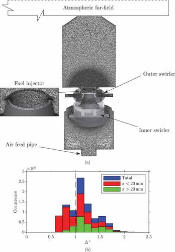
A schematic of the DLR combustor is shown in Figure 1. Dry air at atmospheric pressure and room temperature entered a single plenum and the flow was split through two radial swirlers. The two co-swirling flows entered the combustion chamber through a central nozzle of diameter 15 mm and an annular nozzle with inner and outer diameters of 17 and 25 mm, respectively. Methane was fed through a non-swirling nozzle ring having 72 channels $(0.5\times 0.5\mathrm{m}{\mathrm{m}}^2)$ that were located between the two air nozzles. The mass flow rates of air and methane are denoted using ${\dot{m}}_{\mathrm{a}\mathrm{i}\mathrm{r}}$ and ${\dot{m}}_{\mathrm{C}{\mathrm{H}}_4}$, respectively. The exit planes of the central air and methane nozzles are $4.5\mathrm{m}\mathrm{m}$ below the exit of the annular air nozzle and the entrance to the combustion chamber. This location corresponds to $x=0$, as shown in Figure 1 with the coordinate axes. The combustion chamber had a square cross-section with an internal area of $85\times 85\mathrm{m}{\mathrm{m}}^2$ and a length of $114\mathrm{m}\mathrm{m}$.

Figure 1. Schematic drawing of the gas turbine model combustor (Meier et al., 2006; Weigand et al., 2006).

Laser Doppler Velocimetry (LDV) was used to obtain time-averaged statistics for the three components of velocity at various axial positions across the combustor and laser Raman spectroscopy was used for species, mixture fraction, and temperature measurements. In addition, stereoscopic Particle Image Velocimetry (PIV) was used to capture the instantaneous flow field on a chosen mid-plane, along with Planar Laser Induced Fluorescence (PLIF) of OH radicals (Stöhr et al., 2011). These PLIF images span the width of the combustion chamber up to an axial position of $x=45\mathrm{m}\mathrm{m}$, whereas the PIV measurements were limited to a $30\times 30\mathrm{m}{\mathrm{m}}^2$ region from the exit of the annular air nozzle. The full description of the measurement techniques are outlined by Meier et al. (2006), Weigand et al. (2006), and Stöhr et al. (2011).

The various important parameters for the flame close to blow-off, referred to as flame C, are listed in Table 1. This flame was also seen to be the most thermo-acoustically stable flame, as the pressure oscillation amplitude was weakest out of the three flames investigated experimentally (Steinberg et al., 2012). The flow rates, thermal power, and global equivalence ratio that were used in the experiment are listed in Table 1. The swirl number is defined using a standard formula as written, for example, in the study by Weigand et al. (2006). Under these operating conditions, the flame root was positioned at an average height of approximately $6\mathrm{m}\mathrm{m}$ above the fuel nozzle exit. In addition, the flame was observed to be highly unstable with random sudden lift-off events and the flame base returning to the location of $x\approx 1.5\mathrm{m}\mathrm{m}$, which occurred 1–2 times per second. This lift-off event was observed to reach a height of 30–40 mm and lasted approximately 0.1–0.15 s in the experimental study (Weigand et al., 2006). The stabilised flame and its lift-off events were shown by Stöhr et al. (2011) using the time sequences of the combined high-speed ($5\mathrm{k}\mathrm{H}\mathrm{z}$) PIV and OH–PLIF images.

Table 1. Operating conditions for flame C (Meier et al., 2006; Weigand et al., 2006).

Parameter	Value	Description
${\dot{m}}_{\mathrm{a}\mathrm{i}\mathrm{r}}$	$4.68\mathrm{g}/\mathrm{s}$	Air flow rate through the plenum
${\dot{m}}_{\mathrm{C}{\mathrm{H}}_4}$	$0.15\mathrm{g}/\mathrm{s}$	Methane flow rate through the nozzle
$P_{\mathrm{t}\mathrm{h}}$	$7.6\mathrm{k}\mathrm{W}$	Overall thermal power
$S$	$0.55$	Swirl number
ɸglob	$0.55$	Global equivalence ratio

Numerical modelling framework

Governing equations

Before describing the computational model and boundary conditions for the gas turbine model combustor, an overview of the LES and combustion modelling is first outlined. The filtered conservation equations for mass and momentum are written as

(1) $\frac{\mathrm{\partial }\bar{\rho }}{\mathrm{\partial }t}+\mathrm{\nabla }\cdot (\bar{\rho }\tilde{\mathbf{U}})=0,$(1)

(2) $\text{overline rho {{{rm{D}}widetilde {bf U}} over {{rm{D}}t}} = - nabla overline p+ nabla cdot left({overline } taua - {{overline taua }^r}} right){kern 1pt} ,}$(2)

where $\tilde{\mathbf{U}}$ is the Favre-filtered velocity vector and $\bar{p}$ is the modified filtered pressure, which is the sum of the filtered pressure and $2{\tilde{k}}_{\mathrm{s}\mathrm{g}\mathrm{s}}/3$. The molecular viscous stress tensor and the residual anisotropic stress tensor, denoted using $\overline{\text{taua}}$ and ${\overline{\text{taua}}}^r$, respectively, are modelled using the Boussinesq eddy-viscosity concept (Poinsot and Veynante, 2012). The molecular viscosity is calculated using Sutherland’s Law and the sub-grid eddy viscosity is modelled using the constant Smagorinsky model (Smagorinsky, 1963).

It is known that the flame studied here is lifted and swirl-stabilised. Since the fuel and air enter the combustion chamber through separate inlets, combustion is partially premixed. Hence, the modelling methodology for partially premixed combustion must account for both premixed and non-premixed modes. The combustion modelling framework is based on the partially premixed study by Chen et al. (2017), which has proved to be successful for LES (Chen et al., 2019; Langella et al., 2018). The fuel-air mixing is described using a mixture fraction $\xi$, as defined by Bilger et al. (1990). The reaction progress variable $c$ is used to describe the progress of combustion and for this study, it is defined as the sum of the $\mathrm{C}\mathrm{O}$ and $\mathrm{C}{\mathrm{O}}_2$ mass fractions. This is written as $c=\psi /{\psi }^{\mathrm{e}\mathrm{q}}$, where $\psi =Y_{\mathrm{C}\mathrm{O}}+Y_{\mathrm{C}{\mathrm{O}}_2}$ and the superscript “eq” denotes the equilibrium value for the local mixture.

Furthermore, combustion is an SGS phenomenon and it is essential that the interactions between turbulence and combustion are accurately modelled. In this study, a flamelet model is used to map the thermochemical quantities required for partially premixed combustion. This map uses the first two moments of the mixture fraction and progress variable as the control variables. The thermochemical enthalpy (a form of the energy equation) is used to calculate the temperature. These thermochemical quantities are all obtained from their respective transport equations, which is written as

(3) $\text{bar rho {{{rm{D}}{{widetildevarphii}}} over {{rm{D}}t}} = nabla cdot left( {overline {rho {mathcal {D}}\_{rm eff}}}}}nabla {rm{ }}{bf{widetildevarphii}}} right) + overline {{bf{S}}\_{bf{varphii }}^ + } - overline {{bf{S}}\_{bf{varphii }}^ - },}$(3)

where the vectors of the transported Favre-filtered scalars, sources and sinks are respectively given by

(4) $\widetilde{\text{varphii}}=\left\{\tilde{\xi };{\sigma }_{\xi ,\mathrm{s}\mathrm{g}\mathrm{s}}^2;\tilde{c};{\sigma }_{c,\mathrm{s}\mathrm{g}\mathrm{s}}^2;\tilde{h}\right\},$(4)

(5) $\overline{{\mathbf{S}}_{\text{varphii}}^{+}}=\left\{0;2\frac{{\mu }_T}{\mathrm{S}{\mathrm{c}}_T}|\mathrm{\nabla }\tilde{\xi }{|}^2;\overline{{\dot{\omega }}^{\ast }};2\frac{{\mu }_T}{\mathrm{S}{\mathrm{c}}_T}|\mathrm{\nabla }\tilde{c}{|}^2+2\left(\overline{c{\dot{\omega }}^{\ast }}-\tilde{c}\overline{{\dot{\omega }}^{\ast }}\right);0\right\},$(5)

(6) $\overline{{\mathbf{S}}_{\text{varphii}}^{-}}=\left\{0;2\bar{\rho }{\tilde{\chi }}_{\xi ,\mathrm{s}\mathrm{g}\mathrm{s}};0;2\bar{\rho }{\tilde{\chi }}_{c,\mathrm{s}\mathrm{g}\mathrm{s}};0\right\}.$(6)

The effective diffusivity is the sum of the laminar and turbulent contributions. For the first two moments of $\xi$ and $c$, this is written as $\text{{mathcal D}\_{{rm{eff}}} = {mathcal {D} + {nu\_{it T}}/{rm{S}}{{rm{c}}\_{it T}},,}$, while the effective diffusivity for the enthalpy equation is $\text{{{mathcal {D}\_{{rm{eff}}}} = alpha + {nu \_T}/{rm{P}}{{rm{r}}\_T}}$, where $\alpha$ denotes the molecular thermal diffusivity. The turbulent dimensionless numbers ${\mathrm{S}\mathrm{c}}_T$ and ${\mathrm{P}\mathrm{r}}_T$ are assigned constant values of 0.4 (Pitsch and Steiner, 2000). The remaining unclosed terms in Equations (5) and (6) are the reaction related source terms $\overline{{\dot{\omega }}^{\ast }}$ and $\overline{c{\dot{\omega }}^{\ast }}$, and the SGS scalar dissipation rates ${\tilde{\chi }}_{\xi ,\mathrm{s}\mathrm{g}\mathrm{s}}$ and ${\tilde{\chi }}_{c,\mathrm{s}\mathrm{g}\mathrm{s}}$.

The filtered reaction rate is written as

(7) $\overline{{\dot{\omega }}^{\ast }}=\underset{{\bar{\dot{\omega }}}_{\mathrm{f}\mathrm{p}}}{\underbrace{\bar{\rho }{\int }_0^1{\int }_0^1\frac{\dot{\omega }\left(\eta ,\zeta \right)}{\rho \left(\eta ,\zeta \right)}\tilde{P}\left(\eta ,\zeta \right)\mathrm{d}\eta \mathrm{d}\zeta }}+\underset{{\bar{\dot{\omega }}}_{\mathrm{n}\mathrm{p}}}{\underbrace{\bar{\rho }\tilde{c}{\tilde{\chi }}_{\xi }{\int }_0^1\frac{1}{{\psi }^{\mathrm{e}\mathrm{q}}\left(\eta \right)}\frac{{\mathrm{d}}^2{\psi }^{\mathrm{e}\mathrm{q}}\left(\eta \right)}{\mathrm{d}{\eta }^2}\tilde{P}\left(\eta \right)\mathrm{d}\eta }},$(7)

where the premixed and non-premixed filtered reaction rates are denoted as ${\bar{\dot{\omega }}}_{\mathrm{f}\mathrm{p}}$ and ${\bar{\dot{\omega }}}_{\mathrm{n}\mathrm{p}}$, respectively. The premixed contribution is based on a presumed sub-grid joint PDF approach for the mixture fraction and progress variable using the sample space variables $\eta$ and $\zeta$ for the mixture fraction and progress variable, respectively. This density-weighted PDF is approximated as $\tilde{P}(\eta ,\zeta )\approx {\tilde{P}}_{\beta }(\eta ;\tilde{\xi },{\sigma }_{\xi ,\mathrm{s}\mathrm{g}\mathrm{s}}^2)\times {\tilde{P}}_{\beta }(\zeta ;\tilde{c},{\sigma }_{c,\mathrm{s}\mathrm{g}\mathrm{s}}^2)$ and the shape of the two PDFs is assigned using beta functions. The filtered quantities required for the PDFs are obtained from their respective transport equations, as given in Equation (3). The flamelet reaction rate $\dot{\omega }(\eta ,\zeta )$ is calculated from the unstrained planar laminar premixed flame calculation for different mixture fractions within the flammability limits of the methane-air mixture and this calculation also provides $\rho (\eta ,\zeta )$. The other source term $\overline{c{\dot{\omega }}^{\ast }}$ is determined in a manner similar to ${\bar{\dot{\omega }}}_{\mathrm{f}\mathrm{p}}$.

The non-premixed filtered reaction rate term contains the filtered dissipation rate of the mixture fraction, which is the sum of the resolved and SGS parts according to ${\tilde{\chi }}_{\xi }=\tilde{\mathcal{D}}(\mathrm{\nabla }\tilde{\xi }\cdot \mathrm{\nabla }\tilde{\xi })+{\tilde{\chi }}_{\xi ,\mathrm{s}\mathrm{g}\mathrm{s}}$. The SGS contribution is modelled using a linear relaxation model ${\tilde{\chi }}_{\xi ,\mathrm{s}\mathrm{g}\mathrm{s}}=C_{\xi }({\nu }_T/{\mathrm{\Delta }}^2){\sigma }_{\xi ,\mathrm{s}\mathrm{g}\mathrm{s}}^2$ (Pitsch, 2006). The model constant is $C_{\xi }=2$ and the SGS mixture fraction variance is transported using Equation (3). The filter width is computed as $\mathrm{\Delta }\approx {\mathcal{V}}^{1/3}$, with $\mathcal{V}$ being the volume of the computational cell.

The final term that requires closure is the SGS scalar dissipation rate for $c$. This is modelled using the algebraic expression proposed by Dunstan et al. (2013) and is given as

(8) ${\tilde{\chi }}_{c,\mathrm{s}\mathrm{g}\mathrm{s}}=\mathcal{F}\left[2K_c(\xi )\frac{s_L^0(\xi )}{{\delta }_L^0(\xi )}+\left(C_3-\tau (\xi )C_4\mathrm{D}{\mathrm{a}}_{\mathrm{\Delta }}\right)\left(\frac{2u_{\mathrm{\Delta }}^{\prime }}{3\mathrm{\Delta }}\right)\right]\frac{{\sigma }_{c,\mathrm{s}\mathrm{g}\mathrm{s}}^2}{{\beta }_c},$(8)

with $\mathcal{F}=1-exp\left(-0.75\mathrm{\Delta }/{\delta }_L^0\right)$ being a function to ensure that ${\tilde{\chi }}_{c,\mathrm{s}\mathrm{g}\mathrm{s}}$ approaches zero when $\mathrm{\Delta }/{\delta }_L^0\to 0$. The SGS parameters $\mathrm{D}{\mathrm{a}}_{\mathrm{\Delta }}$, $C_3$, $C_4$, and $K_c$ are described in detail by Dunstan et al. (2013). This model has been successfully used in many previous studies (Chen et al., 2017, 2019; Langella et al., 2018, 2016; Massey et al., 2018). The laminar flame speed $s_L^0$, thermal thickness ${\delta }_L^0$ and the heat release parameter $\tau$, shown in Equation (8), depend on the local mixture fraction (Ruan et al., 2014). These values are obtained from the flamelet calculation, where the heat release parameter is the normalised temperature rise defined as $\tau (\xi )=(T_b(\xi )-T_u)/T_u$, with the subscripts $b$ and $u$ representing fully burnt and unburnt conditions, respectively. The SGS velocity scale $u_{\mathrm{\Delta }}^{\prime }$ is modelled using a scale-similarity approach (Pope, 2000). A value of $7.5$ is used for ${\beta }_c$, following the study by Chen et al. (2019), although ${\beta }_c$ can be evaulated dynamically (Gao et al., 2015; Langella et al., 2015).

The Favre-filtered temperature is obtained using the filtered enthalpy transport equation and is calculated through $\tilde{T}=T_0+(\tilde{h}-{\widetilde{\mathrm{\Delta }h}}_f^0)/{\tilde{c}}_p$. The terms $c_p$ and $\mathrm{\Delta }{h}_f^0$, respectively, represent the effective specific heat capacity at constant pressure and the formation enthalpy of the gas mixture, and the reference temperature is $T_0=298.15\mathrm{K}$. The mixture density is computed using the state equation $\bar{\rho }=\bar{p}\tilde{M}/{\mathrm{\Re }}^0\tilde{T}$, where $\tilde{M}$ represents the Favre-filtered mixture molecular mass and ${\mathrm{\Re }}^0$ is the universal gas constant. The three thermochemical quantities for the mixture ${\widetilde{\mathrm{\Delta }h}}_f^0$, ${\tilde{c}}_p$, and $\tilde{M}$ are calculated similarly to the premixed reaction rate in Equation (7) and are included in the look-up table; this is described in further detail Ruan et al. (2014). The laminar flames used to build the table are computed using Cantera and the GRI-Mech 3.0 chemical mechanism (Goodwin et al., 2017).

Computational details

The computational domain, shown in Figure 2(a), includes an air feed pipe, the plenum, both swirlers and the combustion chamber. A large cylindrical atmospheric far-field is included downstream of the combustion chamber exit to prevent acoustic wave reflection. All of the walls are adiabatic with no-slip conditions, apart from the walls in the streamwise direction of the extended far-field domain, which have slip conditions imposed. The outlet is specified to have zero streamwise gradients for all the variables. The air feed pipe and fuel injector have constant mass flow rate boundary conditions imposed using the values in Table 1 along with a top-hat velocity profile. All 72 fuel injectors are included in the mesh to provide an improved accuracy for the fuel-air mixing. The computational grid consists of 20 million unstructured tetrahedral cells; Chen et al. (2019) conducted a grid sensitivity study and demonstrated that the grid presented here suitably resolved the turbulence and mixing fields. At least two cells adjacent to the wall are within $y^{+}<5$, in order to ensure that the velocity field in those regions is insensitive to the use of a wall model (Chen et al., 2019). Figure 2(b) shows three histograms of the normalised filter width ${\mathrm{\Delta }}^{+}=\mathrm{\Delta }/({\delta }_L^0{)}_{\mathrm{s}\mathrm{t}}$ for the reacting region ($\overline{{\dot{\omega }}^{\ast }}>0$) of the computational domain. The histograms constructed for the cells above and below $x=20\mathrm{m}\mathrm{m}$ are coloured using red and green, respectively, and blue is used to mark the histogram for cells with $\overline{{\dot{\omega }}^{\ast }}>0$ over the entire combustion chamber. In general, it is seen that the grid does not resolve the flame front and hence, combustion is entirely modelled at the SGS.

Figure 2. Compuational grid for the gas turbine model combustor (a) and histograms of the normalised filter width distribution (b), where the cell samples are collected within the reaction region marked using $\overline{{\dot{\omega }}^{\ast }}>0$.

The simulations are performed using OpenFOAM $\mathrm{2.3.0}$, with second-order central difference schemes for the spatial derivatives. A first-order implicit Euler scheme is used for the temporal derivatives and therefore, a small time step of $\mathrm{\Delta }t=0.15\mu \mathrm{s}$ is used to ensure suitable accuracy for the time derivatives and that the CFL number remains below $0.4$ across the whole domain. This low CFL number is required due to the small grid cells near the fuel nozzle (these are of the order ${10}^{-4}\mathrm{m}$) and to ensure numerical stability for the second-order velocity spatial discretisation schemes with no blending factors. A Pressure-based Implicit Splitting of Operators (PISO) method (Issa, 1986) is used and iterated for a maximum of five times within each time step, in order to ensure close coupling between pressure and velocity. This iterative scheme on the PISO algorithm is referred to as the PIMPLE algorithm in OpenFOAM. The simulation for flame C that is presented next was ran on ARCHER, a national high performance computing facility in the United Kingdom. The simulation used 1080 cores, where 1 hr of wall clock time produced statistics for 1 ms of physical time. This case requires around 80 ms of physical time to allow initial transients to pass out of the domain. The time-averaged statistics are computed using samples collected over 24 ms after the initial 80 ms transient period. This 24 ms sample corresponds to roughly 6 flow-through times. Since the lift-off event is observed to begin at approximately 108 ms, the simulation is run for another 45 ms to capture the evolution of the lift-off event.

It should be noted that the SGS reaction rate closure used for this study is flamelets based, which typically assumes that the chemical time scale is shorter than the relevant turbulent time scales. In the context of Reynolds-Averaged Navier–Stokes (RANS) modeling, it is permissible to question whether this combustion model can be used to study flame blow-off mechanisms. However, the situation is different for LES modelling, since many of the fluid time scales, along with their interactions and mutual influences on the scalar fields, are resolved explicitly and captured by the LES equations. In addition, a flame will physically exist if the local mixture is flammable with the right reactedness values. The local mixture value is denoted by the filtered mixture fraction and its SGS variance, whereas the reactedness value is represented by the filtered progress variable and its SGS variance. The influences of strain due to the resolved fluid motion on the evolution of these fields are captured inherently by the LES equations. However, it may be queried as to whether the influence of SGS straining on the flame should be included. The multi-scale analysis of Doan et al. (2017) and Ahmed et al. (2018) demonstrated that turbulent eddies smaller than $2{\delta }_L^0$ to $3{\delta }_L^0$ contribute weakly to the overall straining of the flame. Hence, the unstrained flamelets-based models can be used (provided that the numerical grid satisfies the aforementioned condition) as SGS closure to investigate mechanisms leading to flame blow-off, which are related to the dynamic interaction between the flame and large-scales of motion. These points will become evident from the results presented next.

Results

Reacting flow structures

The axial velocity with streamlines and temperature distributions on the $x-y$ mid-plane are shown in Figure 3(a) and 3(b), respectively. The left-hand side of each figure shows a snapshot of the LES results and the right-hand side shows the time-averaged fields, which are also azimuthally averaged. The nozzle Reynolds number based on the cold inflow and minimum diameter of the outer annulus (25 mm) is approximately $15,000$. An Inner Recirculation Zone (IRZ), which is typical in swirling flows, is seen in Figure 3(a) with a length of approximately 63 mm in the axial direction. This computed value is in excellent agreement with the measured value of 65 mm (Weigand et al., 2006). The high negative axial velocities near $x=0$ at the centreline indicate that the recirculation flow is strong. An Outer Recirculation Zone (ORZ) is also formed at the bottom of the combustion chamber near the walls, since the chamber is confined. The effect of thermal expansion, which can be seen by the high temperatures in Figure 3(b) in the IRZ, also causes the ORZ to be small. It is seen in the left-hand side of Figure 3(a) that there are some instantaneous circular patterns along the inner shear layer (white coloured region) between the IRZ and the inflow stream. These regions of high vorticity magnitude (not shown) correspond to the large-scale coherent structures in the flow.

Figure 3. Distributions of the (a) axial velocity and (b) temperature fields for flame C. The filtered and averaged, in both time and the azimuthal direction, variations are shown on the left- and right-hand sides respectively. The corresponding streamlines are also shown.

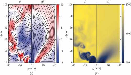
In Figure 3, a strong temperature gradient at the centreline near the bottom of the combustion chamber is shown in the axial direction. This represents the leading edge of the flame and the continuous supply of hot products within the IRZ to this region ensures that the flame stabilizes here and is lifted. Strong temperature gradients are also observed within the large vortex structures, indicating that combustion is also favored within these regions. It should be noted that the large temperature gradient seen within the ORZ near the bottom of the combustion chamber is caused by the hot products attempting to perturb the incoming air stream and hence, there is no flame at this region.

Figure 4 shows typical time-averaged statistics comparisons between the simulation and measurements for three components of the Favre-filtered velocity at different heights from the exit of the annular nozzle. The axial velocity profiles are shown in Figure 4(a), and the radial and azimuthal velocity profiles are shown in Figure 4(b). Some under prediction in the axial and radial velocities is seen in the near field profiles at $x=5\mathrm{m}\mathrm{m}$, but the reverse flow at the centreline is captured well. Moving farther downstream, it is shown that the under prediction in the peak axial velocity continues, as seen in Figure 4(a), and the locations of the local peaks are farther away from the centreline for $x=20$ and $30\mathrm{m}\mathrm{m}$. 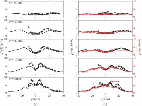There is a small over prediction in the peak radial velocity at $x=20\mathrm{m}\mathrm{m}$ and its radial position is also slightly over predicted. All of these differences suggest that the width of the IRZ at this location is over predicted in the LES. This is caused by the difficulty in capturing the flow separation along the contoured outer-wall of the annular air nozzle (see Figure 1). At the farthest downstream location, the three velocity components are captured well. The corresponding root mean square (rms) values of the three velocity components are shown in Figure 5, where the rms is obtained using only the resolved variance as $⟨{\sigma }_{\mathbf{U}}^2⟩=⟨{\tilde{\mathbf{U}}}^2-⟨\tilde{\mathbf{U}}{⟩}^2⟩$. The position of the local peaks corresponds to the shear layers, where the fluctuations of the velocity are highest. These peak rms positions are sufficiently captured in the LES for all velocity components, except a radial shift in the axial velocity is shown at $x=20$ and $x=30\mathrm{m}\mathrm{m}$, as seen in Figure 4(a) for the mean velocities. Furthermore, the discrepancies seen between the measured data and simulation are partly attributed to including only the resolved fields. The rms axial velocity at $x=5\mathrm{m}\mathrm{m}$ is captured well and the maximum resolved rms value is $70\mathrm{\%}$ of the maximum peak in the measured data, suggesting the grid resolves the flow field satisfactorily.

Figure 4. Comparisons of the time-averaged (a) axial and (b) radial and azimuthal velocities between the measurements (Meier et al., 2006; Weigand et al., 2006) (symbols) and the computations (lines), where the latter results are azimuthally averaged.

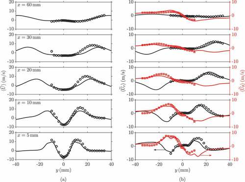
Figure 5. Comparisons of the time-averaged (a) axial and (b) radial and azimuthal rms velocities between the measurements (Meier et al., 2006; Weigand et al., 2006) (symbols) and the computations (lines), where the latter results are azimuthally averaged.

The time-averaged Favre-filtered mixture fraction and temperature profiles are shown in Figure 6(a) and 6(b), respectively. As with the velocity statistics, the agreement between the measured and computed values at the near field is good, especially for the averaged mixture fraction. The temperature at $x=5\mathrm{a}\mathrm{n}\mathrm{d}10\mathrm{m}\mathrm{m}$ along the centreline is under predicted by $13\mathrm{\%}$ and $4\mathrm{\%}$, respectively. This would suggest that the lift-off height for the stabilisation root is over estimated by approximately $10\mathrm{\%}$ in the simulation; this will be discussed in further detail in the next section. Furthermore, the temperature in the region $|y|>20\mathrm{m}\mathrm{m}$ is over predicted by the simulation. However, it is demonstrated in Figure 6(a) that the mixing in the near regions is captured well by the simulation. Thus, the over prediction in temperature in the large radial positions is most possibly due to the adiabatic wall treatment in the LES. Moving farther downstream, it is shown that the agreement between the measurements and the simulation is good, but the temperature in the regions close to the wall ($|y|\ge 30\mathrm{m}\mathrm{m}$), is again over predicted by the simulation at $x=30\mathrm{m}\mathrm{m}$. The over predictions of the near-wall temperature are also seen in the rms temperature profiles in Figure 7(b). The effect of nonadiabatic wall treatment on this flame will be investigated in a future study. There are also some over predictions in the peak mixture fraction rms values in the near field within the jet regions, despite the good agreement for the mean values. This is mainly due to the averaging effects coming from the significantly larger sized Raman measurement probe used (0.6 mm) compared to the LES grid size (0.3 mm) for the near field at $x=5\mathrm{a}\mathrm{n}\mathrm{d}10\mathrm{m}\mathrm{m}$. It can be seen in Figure 7(a) that this effect becomes less influential as the agreement for the rms mixture fraction improves when moving downstream. Nonetheless, the comparisons show that the overall flow and flame structures are well predicted in the LES for this flame, which is close to the lean blow-off limit. This permits further analysis of the LES data, in order to gain physical insights into the unsteady behaviours of this lean swirl flame in the following sections.

Figure 6. Comparisons of the time-averaged (a) mixture fraction and (b) temperature profiles between the measurements (Meier et al., 2006; Weigand et al., 2006) (symbols) and the computations (lines), where the latter results are azimuthally averaged.

Figure 7. Comparisons of the time-averaged (a) rms mixture fraction and (b) rms temperature profiles between the measurements (Meier et al., 2006; Weigand et al., 2006) (symbols) and the computations (lines), where the latter results are azimuthally averaged.

Flame dynamics

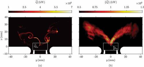
It was observed in the experimental study that this flame experienced random lift-off events and therefore, the flame location and its structure changes significantly, along with the distribution of the heat release rate; these experimental observations are investigated in this subsection. The distributions of the filtered (at an arbitrarily chosen time $\mathrm{t}=104.525\mathrm{m}\mathrm{s}$ ) and time-averaged heat release rate, denoted by the braces, are shown in Figure 8(a) and 8(b). It is shown that the flame has regions of high heat release at a root in the regions close to the bottom of the combustion chamber and within the vortices along the inner shear layer. The time-averaged field in Figure 8(b) shows that the flame brush has a “V” shape and the highest heat release is around the flame root region, where the fresh reactants mix rapidly with the recirculating hot products. This flame root then acts as an ignition source propagating downstream, resulting in an elongated reaction zone along the inner shear layer, as observed in Figure 8(b). It is shown that the average position of the root is at $x=2\mathrm{m}\mathrm{m}$, which corresponds to a lift-off height of $h_{\mathrm{l}\mathrm{o}}=6.5\mathrm{m}\mathrm{m}$ (above the fuel nozzle), as marked in Figure 8(b). This is close to the lift-off height observed in the experiment, which was around 6 mm above the fuel nozzle (Weigand et al., 2006), suggesting that the complex interactions between the flame root and the swirling flow are captured well in the LES.

Figure 8. Distributions of the (a) filtered and (b) time-averaged heat release rate fields on the $x$–$y$ mid-plane.

It was also reported by Stöhr et al. (2011) that during an unstable event, the flame root was extinguished, leading to flame lift-off. The flame then moved back upstream and returned to the location of $h_{\mathrm{l}\mathrm{o}}\approx 6\mathrm{m}\mathrm{m}$. Different flame shapes were seen during the lift-off events and therefore, the distribution of the heat release rate will have changed significantly with time. These phenomena captured in the LES are depicted in Figure 9. The dash-dotted line in Figure 9(a) shows the temporal variation of the heat release rate integrated over the entire combustion chamber, denoted as ${\bar{\dot{Q}}}_{\mathrm{g}\mathrm{l}\mathrm{o}\mathrm{b}}$, for 45 ms, which is an arbitrarily chosen interval that included a lift-off event in the simulation. The volume integrated heat release rate varies with time, but it is close to the thermal power of $P_{\mathrm{t}\mathrm{h}}=7.6\mathrm{k}\mathrm{W}$ for the experiment. However, it is difficult to identify the lift-off event from this quantity. Therefore, it is decided to monitor the temporal variation of the heat release rate integrated over a small volume centred at $x=0$ of size $10\times 20\times 20\mathrm{m}{\mathrm{m}}^3$, as shown in Figure 8. This heat release rate, denoted as ${\bar{\dot{Q}}}_{\mathrm{l}\mathrm{o}}$, is also shown in Figure 9(a), using the solid line, but multiplied by 100 to show on the same scale as the global heat release values. It is evident that the heat release rate in this region changes significantly over the time interval shown. The fluctuation observed for the first 4 ms is due to some initial transients and this heat release rate is large when the flame root comes into the smaller monitoring region. A large drop in ${\bar{\dot{Q}}}_{\mathrm{l}\mathrm{o}}$ is observed until $t=109\mathrm{m}\mathrm{s}$, but since the global heat release rate is large at this time, this suggests that the flame root is moving out of the smaller monitoring region. Some fluctuations in ${\bar{\dot{Q}}}_{\mathrm{l}\mathrm{o}}$ are observed for the time interval $109<t<124\mathrm{m}\mathrm{s}$, suggesting that the flame root is coming into the monitoring region periodically. These fluctuations weaken for the interval $124<t<141\mathrm{m}\mathrm{s}$, which suggests that the flame is outside of the monitoring region. The last part of the sequence $t>141\mathrm{m}\mathrm{s}$ shows that ${\bar{\dot{Q}}}_{\mathrm{l}\mathrm{o}}$ now steadily increases up to the values seen when the flame has an established flame root in the monitoring region and hence, it is suggested that the flame has restabilised.

Figure 9. Time series of the (a) volume integrated heat release rate in the combustion chamber and within the marked volume in Figure 8 and (b) the lift-off height above the fuel nozzle.

The lift-off height, denoted using $h_{\mathrm{l}\mathrm{o}}$ and illustrated in Figure 8(b), is tracked and is based on the minimum height from the fuel injector exit where $\tilde{T}=1500\mathrm{K}$ within a radius of $\mathrm{r}<10\mathrm{m}\mathrm{m}$. This variation is shown in Figure 9(b), where the lift-off height is also averaged over every 4.5 ms and the averaged values are shown using horizontal thick lines. On the whole, the trend seen for the lift-off height is directly linked to ${\bar{\dot{Q}}}_{\mathrm{l}\mathrm{o}}$. After the first window of 4.5 ms, the lift-off height fluctuates up to $t=131\mathrm{m}\mathrm{s}$, since the unstable behaviour and fluctuating heat release rate is caused by the flame root trying to establish itself. However, the averaged lift-off heights are 3–6 mm larger than the height in the first interval of roughly 6 mm. Beyond this time, the averaged lift-off height significantly increases, suggesting that the flame recedes downstream and does not stabilise at the root, which is shown by the low heat release rate seen in this region. The last window of 4.5 ms shows that the average height is very similar to the first window and hence, the flame leading edge is established again at its typical location to give a more stable flame in its typical “V” shape.

The results shown in Figure 9 suggest that there could be some frequency of the transient lift-off event and the flame root returning to its typical location. The duration of the LES is insufficient to estimate this frequency, which will be explored in a future study. However, it is possible to identify two different stages of the flame, as marked in Figure 9(b). Stage 1 denotes a stabilised flame with an established flame root and Stage 2 is the transient lift-off event when the flame root is lost or receding downstream. These two stages of the flame base dynamics are described next.

Stage 1: stabilised flame

This stage corresponds to the situation of having the flame base within the monitoring volume and $h_{\mathrm{l}\mathrm{o}}\approx 6\mathrm{m}\mathrm{m}$, as marked in Figure 9. A comparison of the time series showing the stabilised flame behaviour, arbitrarily chosen from the measurements and the LES, is presented in Figure 10. The filtered reaction rate contours and velocity vectors from the LES are shown in Figure 10(a). The blue and red vectors show the smallest and largest velocity magnitude, respectively, where the values are shown in the legend in Figure 10 and the experimental measurements use the same scale. Figure 10(b) shows the combined PIV and OH–PLIF measurements, where the former is taken across a square region as marked in the top of Figure 10(a). The filtered reaction rate is compared with the OH–PLIF measurements, since the reaction rate is readily available from the LES and clearly marks the flame. The time interval between each simulation frame is 0.375 ms, where the first frame is at $t=104.525\mathrm{m}\mathrm{s}$ (see Figure 9). The total duration of the LES sequence is 1.875 ms, which is similar to the 2 ms duration used for the experimental images, as marked in Figure 10(b).

Figure 10. Time series of the simultaneous (a) filtered reaction rate and velocity vectors (coloured by magnitude) and (b) PIV and OH–PLIF measurements for the flame in Stage 1.

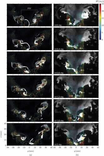
The high reaction rates typically occur in two favored regions, as shown in Figure 10. The first is within small pockets inside of the large coherent structures in the form of a Precessing Vortex Core (PVC), which can be seen by the velocity vectors and their circular patterns, which are present along the “V” shape of the flame. The second region is near the bottom of the combustion chamber, which is the flame root. On the left-hand side of the sequences, it is shown that the flammable mixture is ignited near the bottom at the flame root and the reaction then continues when the structure is convected downstream with time, but ends at around $y=-20\mathrm{m}\mathrm{m}$ in the fourth frame of Figure 10(a). Ignition at the flame root then occurs on the right-hand side in the fifth and sixth frames of Figure 10(a). The repetition rate is controlled by the rotation of the PVC, as described by Stöhr et al. (2011). The frequency for this from the Fourier analysis undertaken by Stöhr et al. (2011) is 510 Hz. It is estimated that the frequency in the simulation by using the sequence shown in Figure 10(a) is approximately 520 Hz. The flame root acts as a source of heat and radicals close the exit of the nozzles and is responsible for the ignition of fresh reactants in the helical zone. It is important that this root remains established, robust and does not recede downstream so that a stable flame exists. This is not guaranteed for flames close to the blow-off limit, which is the case for flame C. Hence, the flame experiences another stage of evolution, which is described next.

Stage 2: lift-off event

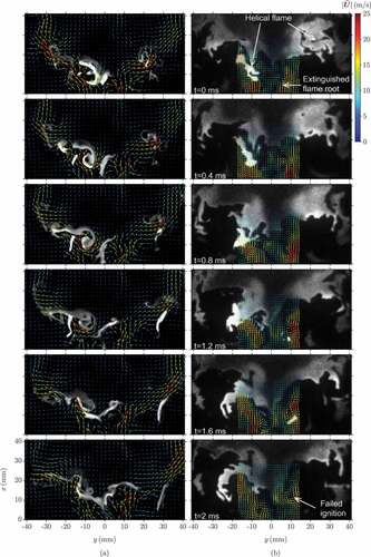
It was suggested in the experimental study by Stöhr et al. (2011) that the lean blow-off event is triggered when the flame root extinguishes and re-ignition does not occur after more than 2 ms. It is also suggested that there must be failed ignition within the vortex centre near the end of the “V” shape after this time period. When both of these events occur, the flame will blow-off.

Figure 11 compares the time sequence of these events from the LES and experiment. The time interval for the simulation between each frame is the same as that used for Figure 10, but the first frame is at $t=111.05\mathrm{m}\mathrm{s}$ (see Figure 9). It is observed that the reaction has been instigated within the vortex in the LES, but the reaction stops before a radial position of 20 mm from the centreline. This is not the case for Stage 1 of the flame, as seen in Figure 10(a), as it is seen that the reaction continues after this radial position. Furthermore, the right-hand side of Figure 11(a) shows that the reaction is very weak and some difficulty of re-ignition is seen around $x=20\mathrm{m}\mathrm{m}$. This is not the case for the experiment, as failed ignition is highlighted in the last frame of Figure 11(b). On the other hand, the reaction at the flame root is very weak in Figure 11(a) and it is seen in the last two frames that the flame root is approximately 4 mm higher up in comparison to its position in Figure 10(a). After the final frame of Figure 11(a), the lift-off height increases significantly, as shown in Figure 9. Therefore, the sequence shown in Figure 11(a) is important and it is suggested that the weak reaction within the vortices and the change in position of the flame root causes the lift-off event to occur. Therefore, an additional investigation into the precursors that lead to the described lift-off event is presented next using the simulation data, since further information can be extrapolated from the LES that is not available in the experiment.

Figure 11. Time series of the simultaneous (a) filtered reaction rate and velocity arrows (coloured by magnitude) and (b) the PIV and OH–PLIF measurements for the event showing the loss of the flame root and local extinction.

Further insights on flame stabilisation

The purpose of this section is to investigate the various physical processes involved in the stabilisation of the flame and the lift-off event seen in Figure 11. The mechanisms involved at the flame root region for Stage 1 of the flame are studied first. The distributions of the filtered mixture fraction and reaction rate on the $x$–$y$ mid-plane are shown in Figure 12(a) and 12(b), respectively. The isolines denote the stoichiometric mixture fraction and the lean and rich flammability limits are approximately $0.028$ and $0.08$, respectively; the dark regions in Figure 12(a) indicate that these mixtures consist of air. Figure 12(b) shows the filtered reaction rate $\overline{{\dot{\omega }}^{\ast }}$ and indicates that the reaction rates are highest along the contour for ${\xi }_{\mathrm{s}\mathrm{t}}$, specifically near the centreline. This typical behaviour is seen during a continuous sequence of the flame in Stage 1, which is stabilised by the PVC. Although the local mixture is stoichiometric, such a high reaction rate is not seen in the locations farther downstream. This implies that the stronger flame located at the base provides the heat and radicals required for flame stabilisation and the “V” shaped flame brush.

Figure 12. Distributions of the (a) filtered mixture fraction and (b) reaction rate for the flame in Stage 1 at t = 104.525 ms. The isolines denote the stoichiometric mixture fraction value of ${\xi }_{\mathrm{s}\mathrm{t}}=0.055$.

Figure 13 shows the filtered mixture fraction and reaction rate distributions for two instances ($t=108.05\mathrm{a}\mathrm{n}\mathrm{d}111.05\mathrm{m}\mathrm{s}$), which are early into Stage 2 of the flame. As seen in Figure 9, the lift-off height increases and the heat release rate in the flame root region decreases after both of these instances. The mixture fraction and reaction rate fields for $t=108.05\mathrm{m}\mathrm{s}$ are shown in Figure 13(a) and 13(b), respectively. On the right-hand side of Figure 13(b), there is no reaction along the stoichiometric mixture fraction line and the reaction rate is very weak in comparison to the reaction rate field in Figure 12(b). This is caused by the air entrainment, leading to the mixture fraction being lower than the lean flammability limit of $0.028$. Although there are local stoichiometric mixtures around $x=7\mathrm{m}\mathrm{m}$, there is no reaction because of the surrounding cold mixtures. This causes the flame to move away in the radial direction on the right-hand side of the domain and leads to the sudden drop of ${\bar{\dot{Q}}}_{\mathrm{l}\mathrm{o}}$ that is seen in Figure 9(a). Consequently, the flame root recedes downstream, which is shown by the increasing lift-off height around $t=108\mathrm{m}\mathrm{s}$ in Figure 9(b).

Figure 13. Distributions of the (a) filtered mixture fraction and (b) reaction rate prior to the lift-off event at $t=108.05\mathrm{m}\mathrm{s}$. The frames (c) and (d) respectively show the filtered mixture fraction and reaction rate at $t=111.05\mathrm{m}\mathrm{s}$.

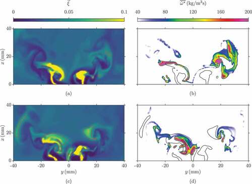
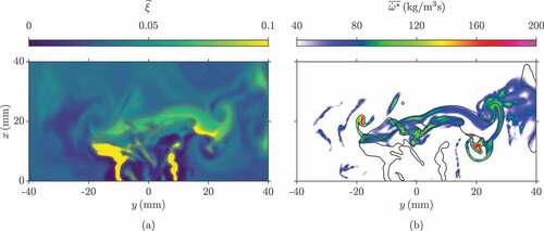
The mixture fraction and reaction rate fields at $t=111.05\mathrm{m}\mathrm{s}$ are shown in Figures 13(c) and 13(d), respectively. It is seen that a pocket of rich mixture is present along the centreline near the bottom of the combustion chamber within the PVC. This causes the flame to move to a higher position and therefore, the flame root is shifted from its typical position, which initiates the lift-off event.

Figure 14 shows the filtered mixture fraction and reaction rate at $t=138.5\mathrm{m}\mathrm{s}$, which is the point in time where the maximum lift-off height is observed, as shown in Figure 9(b). It is seen here that there is a large island of rich mixture above the fuel nozzle and the flame root is not present. The reaction rate is distributed across a large region and with weaker burning, which is dissimilar to the higher reaction rates that are concentrated in smaller regions, as seen in Figure 12. The reaction is weaker in the monitoring region and causes lower values of ${\bar{\dot{Q}}}_{\mathrm{l}\mathrm{o}}$, as seen in Figure 9(a). The mixture fraction distribution in Figure 14(a) shows that the local mixture in this region is typically below the lean flammability limit and therefore, the flame leading edge cannot propagate upstream toward its location observed in Stage 1. Hence, these results show that the large-scale events controlling the fuel-air mixing and the proximity of flammable mixture and hot products control the flame lift-off events. Further analysis is required to understand these in detail and to explain why the lift-off height moves toward its value in Stage 1, as seen in Figure 9(b). A future study will provide these insights and determine if these influences are linked to the complete blow-off of the flame.

Figure 14. Distributions of the (a) filtered mixture fraction and (b) reaction rate for the flame at the maximum lift-off height ($t=138.5\mathrm{m}\mathrm{s}$).

Conclusions

A flame close to the lean blow-off limit in a gas turbine model combustor is simulated using LES. A presumed probability density function approach with flamelets is used as closure for the filtered reaction rate to mimic the SGS combustion process. The statistics for the velocity, mixture fraction and temperature obtained from the simulation compare well with measured values. Good comparisons are also observed for the rms statistics. These validations permit investigation of the numerical data in further detail to gather insights into the behaviour of the flame stabilisation location inside the combustor. This analysis identified two distinct stages for the evolution of flame root. In the first stage, the flame is anchored by its stable and robust root located near the centreline in the near field of the burner and this led to a “V” shaped flame brush (time averaged flame) as observed in the experiment. This is verified by comparing stereo–PIV and OH–PLIF sequences with LES results. It is observed in the LES that the entrainment of inflammable mixture into the flame region within the IRZ leads to the loss of the flame root and initiated the lift-off events in the second stage. The duration of the lift-off event is observed to be approximately 30 ms and the flame is found to be positioned downstream during this event. This flame then moves upstream toward its location observed in Stage 1 of the flame. These two stages are observed to switch from one to the other, as observed in the experiment. This switching is caused by the entrainment of air and weaker mixtures into the flame region created by the unsteady fuel-air mixing phenomena, which are governed by both large-scale eddy motions and small-scale mixing processes. Further analysis is required to distinguish the role of these two processes that lead to flame blow-off and the observations from this study will be followed up in a future study. The role of heat loss, as well as its influence on the flamelet chemistry, and the global equivalence ratio on the flame lift-off events leading to complete blow-off will be explored.

Acknowledgments

J. C. Massey acknowledges the financial support from the EPSRC provided through a doctoral training award (grant no. RG80792). The additional support from Rolls Royce plc. is also acknowledged. Z. X. Chen and N. Swaminathan acknowledge the financial support from Mitsubishi Heavy Industries, Ltd., Japan. Thanks are given to M. Stöhr and W. Meier for providing the experimental data and also for the fruitful discussions. This work used the ARCHER UK National Supercomputing Service (https://www.archer.ac.uk) with the resources provided by the UKCTRF.

Additional information

Funding

This work was supported by the Engineering and Physical Sciences Research Council, UK.

References

- Ahmed, U., Doan, N.A.K., Lai, J., Klein, M., Chakraborty, N., and Swaminathan, N. 2018. Multiscale analysis of head-on quenching premixed turbulent flames. Phys. Fluids, 30, 105102. doi:10.1063/1.5047061
- Barlow, R.S., and Frank, J.H. 1998. Effects of turbulence on specific mass fractions in methane/air jet flames. Symp. (Int.) Combust., 27(1), 1087–1095. doi:10.1016/S0082-0784(98)80510-9
- Barlow, R.S., Meares, S., Magnotti, G., Cutcher, H., and Masri, A.R. 2015. Local extinction and near-field structure in piloted turbulent CH4/air jet flames with inhomogeneous inlets. Combust. Flame, 162(10), 3516–3540. doi:10.1016/j.combustflame.2015.06.009
- Benim, A.C., Iqbal, S., Meier, W., Joos, F., and Wiedermann, A. 2017. Numerical investigation of turbulent swirling flames with validation in a gas turbine model combustor. Appl. Therm. Eng., 110, 202–212. doi:10.1016/j.applthermaleng.2016.08.143
- Bilger, R.W., Stårner, S.H., and Kee, R.J. 1990. On reduced mechanisms for methane-air combustion in nonpremixed flames. Combust. Flame, 80(2), 135–149. doi:10.1016/0010-2180(90)90122-8
- Cavaliere, D.E., Kariuki, J., and Mastorakos, E. 2013. A comparison of the blow-off behaviour of swirl-stabilized premixed, non-premixed and spray flames. Flow Turbul. Combust, 91(2), 347–372. doi:10.1007/s10494-013-9470-z
- Chen, Z., Ruan, S., and Swaminathan, N. 2017. Large Eddy Simulation of flame edge evolution in a spark-ignited methane-air jet. Proc. Combust. Inst, 36(2), 1645–1652. doi:10.1016/j.proci.2016.06.023
- Chen, Z.X., Swaminathan, N., Stöhr, M., and Meier, W. 2019. Interaction between self-excited oscillations and fuel-air mixing in a dual swirl combustor. Proc. Combust. Inst, 37(2), 2325–2333. doi:10.1016/j.proci.2018.08.042
- Dally, B.B., Masri, A.R., Barlow, R.S., and Fiechtner, G.J. 1998. Instantaneous and mean compositional structure of bluff-body stabilized nonpremixed flames. Combust. Flame, 114(1–2), 119–148. doi:10.1016/S0010-2180(97)00280-0
- Doan, N.A.K., Swaminathan, N., and Chakraborty, N. 2017. Multiscale analysis of turbulence-flame interaction in premixed flames. Proc. Combust. Inst, 36(2), 1929–1935. doi:10.1016/j.proci.2016.07.111
- Donini, A.M., Bastiaans, R.J., van Oijen, J.A., and de Goey, L.P.H. 2017. A 5-D implementation of FGM for the large eddy simulation of a stratified swirled flame with heat loss in a gas turbine combustor. Flow Turbul. Combust, 98(3), 887–922. doi:10.1007/s10494-016-9777-7
- Driscoll, J.F. 2011. Future directions and applications of lean premixed combustion. In Turbulent Premixed Flames (Eds. Swaminathan, N., and Bray, K.N.C.), chap. 5. pp. 378–396. Cambridge, UK: Cambridge University Press.
- Dunstan, T.D., Minamoto, Y., Chakraborty, N., and Swaminathan, N. 2013. Scalar dissipation rate modelling for large eddy simulation of turbulent premixed flames. Proc. Combust. Inst, 34(1), 1193–1201.
- Feikema, D., Chen, R.-H., and Driscoll, J.F. 1991. Blowout of nonpremixed flames: maximum coaxial air velocities achievable, with and without swirl. Combust. Flame, 86(4), 347–358. doi:10.1016/0010-2180(91)90128-x
- Galindo, S., Salehi, F., Cleary, M.J., and Masri, A.R. 2017. MMC-LES simulations of turbulent piloted flames with varying levels of inlet inhomogeneity. Proc. Combust. Inst, 36(2), 1759–1766. doi:10.1016/j.proci.2016.07.055
- Gao, Y., Chakraborty, N., and Swaminathan, N. 2015. Dynamic closure of scalar dissipation rate for Large Eddy Simulations of turbulent premixed combustion: a direct numerical simulations analysis. Flow Turbul. Combust, 95(4), 775–802. doi:10.1007/s10494-015-9631-3
- Garmory, A., and Mastorakos, E. 2011. Capturing localised extinction in Sandia Flame F with LES-CMC. Proc. Combust. Inst, 33(1), 1673–1680. doi:10.1016/j.proci.2010.06.065
- Gicquel, L.Y.M., Staffelbach, G., and Poinsot, T. 2012. Large Eddy Simulations of gaseous flames in gas turbine combustion chambers. Prog. Energy Combust. Sci, 38(6), 782–817. doi:10.1016/j.pecs.2012.04.004
- Goodwin, D.G., Moffat, H.K., and Speth, R.L. 2017 Cantera: an Object-oriented Software Toolkit for Chemical Kinetics, Thermodynamics, and Transport Processes.
- Ihme, M., and Pitsch, H. 2008. Prediction of extinction and reignition in nonpremixed turbulent flames using a flamelet/progress variable model: 2. Application in LES of Sandia flames D and E. Combust. Flame, 155(1–2), 90–107. doi:10.1016/j.combustflame.2008.04.001
- Issa, R.I. 1986. Solution of the implicitly discretised fluid flow equations by operator-splitting. J. Comput. Phys, 62(1), 40–65. doi:10.1016/0021-9991(86)90099-9
- Jones, W.P., and Prasad, V.N. 2010. Large Eddy Simulation of the Sandia Flame Series (D–F) using the Eulerian stochastic field method. Combust. Flame, 157(9), 1621–1636. doi:10.1016/j.combustflame.2010.05.010
- Kronenburg, A., and Kostka, M. 2005. Modeling extinction and reignition in turbulent flames. Combust. Flame, 143(4), 342–356. doi:10.1016/j.combustflame.2005.08.021
- Langella, I., Chen, Z.X., Swaminathan, N., and Sadasivuni, S.K. 2018. Large-Eddy Simulation of reacting flows in industrial gas turbine combustor. J. Propuls. Power, 34(5), 1269–1284. doi:10.2514/1.b36842
- Langella, I., Swaminathan, N., Gao, Y., and Chakraborty, N. 2015. Assessment of dynamic closure for premixed combustion large eddy simulation. Combust. Theory. Model, 19(5), 628–656. doi:10.1080/13647830.2015.1080387
- Langella, I., Swaminathan, N., and Pitz, R.W. 2016. Application of unstrained flamelet SGS closure for multi-regime premixed combustion. Combust. Flame, 173, 161–178. doi:10.1016/j.combustflame.2016.08.025
- Ma, P.C., Wu, H., Labahn, J.W., Jaravel, T., and Ihme, M. 2019. Analysis of transient blow-out dynamics in a swirl-stabilized combustor using large-eddy simulations. Proc. Combust. Inst, 37(4), 5073–5082. doi:10.1016/j.proci.2018.06.066
- Masri, A.R. 2015. Partial premixing and stratification in turbulent flames. Proc. Combust. Inst, 35(2), 1115–1136. doi:10.1016/j.proci.2014.08.032
- Massey, J.C., Langella, I., and Swaminathan, N. 2018. Large Eddy Simulation of a bluff body stabilised premixed flame using flamelets. Flow Turbul. Combust, 101(4), 973–992. doi:10.1007/s10494-018-9948-9
- Meares, S., and Masri, A.R. 2014. A modified piloted burner for stabilizing turbulent flames of inhomogeneous mixtures. Combust. Flame, 161(2), 484–495. doi:10.1016/j.combustflame.2013.09.016
- Meier, W., Duan, X.R., and Weigand, P. 2006. Investigations of swirl flames in a gas turbine model combustor: II. Turbulence-chemistry interactions. Combust. Flame, 144(1–2), 225–236. doi:10.1016/j.combustflame.2005.07.009
- Pitsch, H. 2006. Large-Eddy Simulation of turbulent combustion. Annu. Rev. Fluid Mech, 38(1), 453–482. doi:10.1146/annurev.fluid.38.050304.092133
- Pitsch, H., and Steiner, H. 2000. Large-eddy simulation of a turbulent piloted methane/air diffusion flame (Sandia flame D). Phys. Fluids, 12(10), 2541–2554. doi:10.1063/1.1288493
- Poinsot, T., and Veynante, D. 2012. Theoretical and Numerical Combustion, 3rd. France, (n.p.).
- Pope, S.B. 2000. Turbulent Flows, Cambridge University Press, Cambridge, UK.
- Ruan, S., Swaminathan, N., and Darbyshire, O. 2014. Modelling of turbulent lifted jet flames using flamelets: a priori assessment and a posteriori validation. Combust. Theory. Model, 18(2), 295–329. doi:10.1080/13647830.2014.898409
- See, Y.C., and Ihme, M. 2015. Large eddy simulation of a partially-premixed gas turbine model combustor. Proc. Combust. Inst, 35(2), 1225–1234 doi:10.1016/j.proci.2014.08.006.
- Shanbhogue, S.J., Husain, S., and Lieuwen, T.C. 2009. Lean blowoff of bluff body stabilized flames: scaling and dynamics. Prog. Energy Combust. Sci, 35(1), 98–120. doi:10.1016/j.pecs.2008.07.003
- Smagorinsky, J. 1963. General circulation experiments with the primitive equations. Mon. Weather Rev, 91(3), 99–164. doi:10.1175/1520-0493(1963)091<0099:gcewtp>2.3.co;2
- Steinberg, A.M., Boxx, I., Stöhr, M., Meier, W., and Carter, C.D. 2012. Effects of flow structure dynamics on thermoacoustic instabilities in swirl-stabilized combustion. AIAA J, 50(4), 952–967. doi:10.2514/1.j051466
- Stöhr, M., Boxx, I., Carter, C., and Meier, W. 2011. Dynamics of lean blowout of a swirl-stabilized flame in a gas turbine model combustor. Proc. Combust. Inst, 33(2), 2953–2960. doi:10.1016/j.proci.2010.06.103
- Syred, N. 2006. A review of oscillation mechanisms and the role of the precessing vortex core (PVC) in swirl combustion systems. Prog. Energy Combust. Sci, 32(2), 93–161. doi:10.1016/j.pecs.2005.10.002
- Wandel, A.P., and Lindstedt, R.P. 2013. Hybrid multiple mapping conditioning modeling of local extinction. Proc. Combust. Inst, 34(1), 1365–1372. doi:10.1016/j.proci.2012.07.073
- Weigand, P., Meier, W., Duan, X.R., Stricker, W., and Aigner, M. 2006. Investigations of swirl flames in a gas turbine model combustor: I. Flow field, structures, temperature, and species distributions. Combust. Flame, 144(1–2), 205–224. doi:10.1016/j.combustflame.2005.07.010
- Wu, H., and Ihme, M. 2016. Compliance of combustion models for turbulent reacting flow simulations. Fuel, 186, 853–863. doi:10.1016/j.fuel.2016.07.074
- Xu, J., and Pope, S.B. 2000. PDF calculations of turbulent nonpremixed flames with local extinction. Combust. Flame, 123(3), 281–307. doi:10.1016/s0010-2180(00)00155-3
- Zhang, H., Garmory, A., Cavaliere, D.E., and Mastorakos, E. 2015. Large Eddy Simulation/Conditional moment closure modeling of swirl-stabilized non-premixed flames with local extinction. Proc. Combust. Inst, 35(2), 1167–1174. doi:10.1016/j.proci.2014.05.052
- Zhang, H., and Mastorakos, E. 2016. Prediction of global extinction conditions and dynamics in swirling non-premixed flames using LES/CMC Modelling. Flow Turbul. Combust, 96(4), 863–889. doi:10.1007/s10494-015-9689-y
- Zhang, H., and Mastorakos, E. 2018. LES/CMC modelling of a gas turbine model combustor with quick fuel mixing. Flow. Turbul. Combust, (In Press). 1–22. doi:10.1007/s10494-018-9988-1