Analysis of Markers for Combustion Mode and Heat Release in MILD Combustion Using DNS Data

ABSTRACT

Various commonly used markers for heat release are assessed using direct numerical simulation (DNS) data for Moderate or Intense Low-oxygen Dilution (MILD) combustion to find their suitability for non-premixed MILD combustion. The laser-induced fluorescence (LIF) signals of various markers are synthesized from the DNS data to construct their planar (PLIF) images which are compared to the heat release rate images obtained directly from the DNS data. The local OH values in heat releasing regions are observed to be very small compared to the background level coming from unreacted mixture diluted with exhaust gases. Furthermore, these values are very much smaller compared to those in burnt regions. This observation rises questions on the use of OH-PLIF for MILD combustion. However, the chemiluminescent image obtained using $\mathrm{O}{\mathrm{H}}^{\ast }$ is shown to correlate well with the heat release. Two scalar-based PLIF markers, $\left(\mathrm{O}\mathrm{H}\times \mathrm{C}{\mathrm{H}}_2\mathrm{O}\right)$ and $\left(\mathrm{H}\times \mathrm{C}{\mathrm{H}}_2\mathrm{O}\right)$, correlate well with the heat release. Flame index (FI) and chemical explosive mode analyses (CEMA) are used to identify premixed and non-premixed regions in MILD combustion. Although there is some agreement between the CEMA and FI results, large discrepancies are still observed. The schlieren images deduced from the DNS data showed that this technique can be used for a quick and qualitative identification of MILD combustion before applying expensive laser diagnostics.

KEYWORDS:

• Direct numerical simulation (DNS)
• MILD combustion
• PLIF-signal
• heat release rate marker
• schlieren

Introduction

Considerable progress has been made since 1980s on turbulence–combustion interaction, turbulent combustion modeling (Pope, 2013) and large eddy simulations of reacting flows in practical engines with complex geometries (Menon, 2018). This advancement has helped to find effective solutions to improve the engine efficiency, reduce pollutants emissions and thereby to find ways to design “greener” combustion devices which are friendlier to the environment. Among potential green combustion modes, Moderate or Intense Low-oxygen Dilution (MILD) combustion has gained significant attention because of its ability to reduce pollutants emissions and increase efficiency (Cavaliere and de Joannon, 2004; Wünning and Wünning, 1997). The efficiency gain comes from the energy recovered by recirculating hot gases and the emissions reduction is because of the reduced temperature rise and oxygen level in the combustion zone. This mode of combustion is said to occur when the reactant temperature, $T_r$, is higher than the reference auto-ignition temperature, $T_{ign}$, for a given fuel–air mixture and the temperature rise, $\mathrm{\Delta }T=\left(T_p-T_r\right)$, is smaller than $T_{ign}$ (Cavaliere and de Joannon, 2004). These two conditions are typically achieved by diluting the fuel–air mixture with exhaust gases so that the oxygen level is typically below 5% by volume.

The physics of MILD combustion is quite challenging to unravel because of the strong role of chemical kinetics. It was shown to have specific features such as the absence of a visible flame and spatially distributed heat release resulting in homogeneous temperature fields, which are atypical of conventional turbulent combustion (de Joannon et al., 2000; Katsuki and Hasegawa, 1998; Minamoto and Swaminathan, 2014; Ozdemir and Peters, 2001; Sorrentino et al., 2016). Indeed, conventional combustion has radicals such as OH concentrated in thin regions with large heat release rate (HRR) leading to strong gradients. Many past studies demonstrated that the HRR structures in premixed and non-premixed conventional combustions can be discerned using laser diagnostics (Balachandran et al., 2005; Fayoux et al., 2005; Kiefer et al., 2009; Li et al., 2010; Nguyen and Paul, 1996; Paul and Najm, 1998; Richter et al., 2005; Rosell et al., 2017; Tanahashi et al., 2005). However, the applicability of these diagnostics to combustion under MILD conditions is unclear since the heat releasing regions in MILD combustion appear different from those in conventional combustion. Furthermore, radicals such as OH, CH and HCO used commonly as HRR markers are present in unreacted mixture of MILD combustion because of the dilution using exhaust gases containing these species. Since the temperature rise across the reaction zones in MILD combustion is typically small, the increase in these radicals level above their background (non-reacting mixture) values may be insufficient for an unambiguous identification.

Also, views arising from OH-PLIF imaging of MILD combustion differ and seem to suggest that OH may not be a reliable marker for HRR. For example, OH-PLIF imaging of MILD combustion in a jet-in-hot-coflow (JHC) or a furnace showed thin regions of OH with a clear peak and strong gradients (Dally et al., 2004; Duwig et al., 2012; Medwell et al., 2007; Ozdemir and Peters, 2001; Plessing et al., 1998). On the other hand, Medwell et al. (2009) observed that there is a decrease in OH concentration with an increase in $\mathrm{C}{\mathrm{H}}_2\mathrm{O}$ in MILD reaction zones compared to the conventional combustion. This raises some questions on the use of OH as a HRR marker for MILD combustion. Moreover, the regions captured in OH-PLIF may or may not correspond to heat releasing regions in MILD combustion because the unreacted mixture also contains OH. Indeed, some discrepancies were observed between OH and OH* in another study (Sidey et al., 2014), suggesting that OH may not necessarily coincide with primary heat release under MILD conditions. However, the $\mathrm{O}{\mathrm{H}}^{\ast }$ chemiluminescent signal is known to correspond well to HRR zones and their gross features, but it is inadequate to capture the fine features of these zones required for model development.

Past DNS studies investigated the adequacy of commonly used HRR chemical markers and suggested that two-scalar markers such as $\left(\mathrm{O}\mathrm{H}\times \mathrm{C}{\mathrm{H}}_2\mathrm{O}\right)$ or $\left(\mathrm{H}\times \mathrm{C}{\mathrm{H}}_2\mathrm{O}\right)$ rather than a single scalar were good in identifying HRR regions in MILD combustion (Chi et al., 2018; Minamoto and Swaminathan, 2014; Nikolaou and Swaminathan, 2014; Wabel et al., 2018). However, these studies are for premixed combustion under either conventional or MILD conditions. Here, our interest is to extend those assessments of HRR markers for MILD combustion with mixture fraction variation using DNS data of Doan et al. (2018). This specific interest is because the inception of MILD combustion does not follow the classical routes due to the chemical kinetic role of radicals present in the unreacted mixture as has been shown by Doan and Swaminathan (2019). Also, the presence of both premixed and non-premixed modes in MILD combustion with mixture fraction variation was shown by Doan et al. (2018) using the Flame Index (FI) analysis (Briones et al., 2006; Yamashita et al., 1996). Recently, Hartl et al. (2018) suggested that the chemical explosive mode analysis (CEMA) of Lu et al. (2010) can be used to distinguish premixed from non-premixed regions in partially premixed combustion. Hence, a comparative analysis using the above two, FI and CEMA, techniques is of interest here. Furthermore, MILD combustion is expected to give nearly homogeneous temperature and density fields and thus, the schlieren imaging could be used to distinguish combustion under conventional and MILD conditions. This will also be explored here.

This paper is organized as follows.  The methodology used to conduct the DNS is briefly presented in the next section. The adequacy of some HRR markers and the comparison between the CEMA and FI analyses to distinguish non-premixed from premixed combustion are then discussed in the Result section. Additionally, the analysis using numerical schlieren is investigated. A summary of the main findings is finally provided in the final section.

DNS of MILD combustion

The DNS data of Doan et al. (2018) are of non-premixed MILD combustion of methane–air mixture diluted with recirculated exhaust gases at atmospheric pressure inside a cube of size $L_x\times L_y\times L_z=10\times 10\times 10$ mm${ }^3$. The procedures used to conduct the DNS are illustrated in Figure 1. Details of these procedures are described by Doan et al. (2018) and a brief summary is provided below for the sake of completeness. The initial and inflowing fields of mixture fraction, $Z$, reaction progress variable, $c$, scalar mass fractions, $Y_{\alpha }$, and velocity fields, $u_i$, were generated in five preprocessing steps, marked as steps 1 to 5 in Figure 1.

Figure 1. Schematic illustration of the DNS steps followed for the non-premixed MILD combustion of methane and air diluted with recirculated exhaust gases (from Doan et al. (2018)).

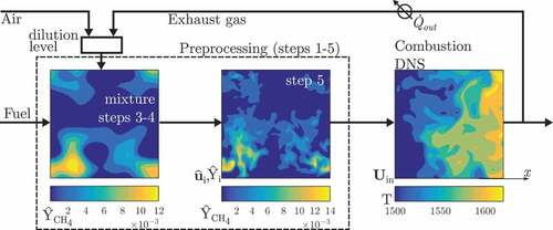
The required turbulence field was obtained in step 1 by simulating a decaying homogeneous isotropic turbulence. Laminar premixed flames under MILD conditions with a reactant temperature of $T_r=1500$ K were computed for various $Z$ values and the scalar mass fractions are tabulated as a function of $Z$ and $c$ in step 2. An initial turbulent mixture fraction, $\hat{Z}$, and reaction progress variable, $\hat{c}$, were constructed with prescribed means, $⟨Z⟩$ and $⟨c⟩$, and length scales ${\mathrm{\ell }}_Z$ and ${\mathrm{\ell }}_c$ in step 3. The symbol $⟨\cdot ⟩$ means quantities averaged over the entire computational volume. The mixture fraction definition of Bilger et al. (1990) was used for $Z$ and the reaction progress variable was based on fuel mass fraction. The species mass fractions $Y_{\alpha }(c,Z)$ obtained in step 2 were mapped onto $\hat{Z}$ and $\hat{c}$ fields in step 4. The turbulence from step 1 and scalar fields from step 4 were then allowed to interact in step 5 for about 40 µs, which is approximately one large eddy turnover time of the initial turbulence field of step 1. This time is much shorter than the lowest reference ignition delay time, which is about 5 ms, for the methane–air mixture conditions considered for this study but long enough to ensure that the scalar and turbulent flow fields have interacted sufficiently before the combustion begins. This ignition delay time was computed using a PSR configuration with fuel–air mixtures diluted with only $\mathrm{C}{\mathrm{O}}_2$, ${\mathrm{N}}_2$ and ${\mathrm{H}}_2\mathrm{O}$ without radical species as normally done for reference ignition delay time calculation. However, there are radical species present in the mixture and thus the actual delay time can be shorter than the reference value of 5 ms. If one uses the volume-averaged values of the various species from the step 4 for the PSR calculation then the $c_T$ value increases by about 10% over a time of 140 µs. This time is sufficiently larger than the mixing time of 40 µs used in the step 5. Also, this delay time is shorter than the residence time.

One could also use other canonical configurations such as a PSR or a counterflow flame instead of a freely propagating premixed flame for step 2 of the preprocessing stage described above to obtain the various scalar fields as a function of Z and c. However, it has been shown by Doan (2018) that $Y_{\alpha }(c,Z)$ does not vary unduly for these configurations.

The scalar fields obtained at the end of step 5 included unburnt ($c=0$), burnt ($c=1$) and partially burnt (intermediate values of $c$) mixtures with equivalence ratio, $\hat{\varphi }=\hat{Z}\left(1-{\hat{Z}}_{st}\right)/\left({\hat{Z}}_{st}\left(1-\hat{Z}\right)\right)$, where $Z_{st}$ is the stoichiometric mixture fraction, varying from 0 to 10 inside the computational domain. These preprocessed fields were then used as the initial and inflowing conditions for the MILD combustion DNS in the second stage as shown in Figure 1. Further details can be found in Doan et al. (2018).

Three cases were simulated by Doan et al. (2018) and their details are given in Tables 1 and 2. The first two cases, AZ1 and AZ2, used the same oxidizer with 3.5% ${\mathrm{O}}_2$ (by volume) but differed in the length scale ratio, ${\mathrm{\ell }}_c/{\mathrm{\ell }}_Z$. The third case BZ1 had more diluted oxidizer (2% of ${\mathrm{O}}_2$) and the same length scale ratio as AZ1, see Table 1. The case of ${\mathrm{\ell }}_c/{\mathrm{\ell }}_Z>1$ was not considered because the mixture fraction mixing length scales are generally larger than the chemical length scales such as the flame thickness or ignition kernel size at $T_r$ as large as 1500 K. All cases had a similar turbulence field with an integral length scale of ${\mathrm{\Lambda }}_0\approx 1.42\mathrm{m}\mathrm{m}$ and root-mean square value of $u^{\prime }\approx 16.66\mathrm{m}/\mathrm{s}$ for the velocity fluctuations. This yielded turbulence and Taylor microscale Reynolds numbers of $\mathrm{R}{\mathrm{e}}_t\approx 96$ and $\mathrm{R}{\mathrm{e}}_{\lambda }\approx 34.73$ respectively.

Table 1. Oxidizer composition for the initial MILD mixture.

Case	$X_{{\mathrm{O}}_2,ox}$	$X_{{\mathrm{H}}_{2}O,ox}$	$X_{\mathrm{C}{O}_2,ox}$	$X_{{\mathrm{N}}_2,ox}$
AZ1-2	0.035	0.134	0.067	0.764
BZ1	0.020	0.46	0.073	0.761

Table 2. MILD combustion DNS initial conditions.

Case	${\mathrm{\Lambda }}_0/{\mathrm{\ell }}_Z$	$⟨X_{{\mathrm{O}}_2}⟩$	$X_{{\mathrm{O}}_2}^{\mathrm{m}\mathrm{a}\mathrm{x}}$	${\mathrm{\ell }}_c/{\mathrm{\ell }}_Z$	$⟨Z⟩$	$Z_{st}$	${\sigma }_Z^2$	$⟨c⟩$	${\sigma }_c^2$
AZ1	0.60	0.0270	0.035	0.77	0.008	0.010	0.00007	0.56	0.068
AZ2	0.79	0.0285	0.035	0.99	0.008	0.010	0.00011	0.56	0.078
BZ1	0.60	0.0160	0.020	0.77	0.0046	0.0058	0.00003	0.56	0.068

The numerical domain was specified to have inflow and non-reflecting outflow boundary conditions in the $x$-direction and periodic conditions in the transverse, $y$ and $z$, directions. The numerical domain was discretized using uniformly distributed $512\times 512\times 512$ grid points to ensure that all chemical and turbulence length scales were resolved (Doan et al., 2018). A combination of Smooke and Giovangigli (1991) and Bilger et al. (1990) mechanisms for methane–air combustion was used for the combustion kinetics along with $\mathrm{O}{\mathrm{H}}^{\ast }$ chemistry from Kathrotia et al. (2012). The resulting mechanism involved 19 species and 58 reactions, and balanced the accuracy and computational cost appropriately by giving a good agreement for the measured values of the laminar flame speeds and ignition delay times. Details and validation of this mechanism are discussed by Doan et al. (2018).

The numerical code SENGA2 was used to solve the fully compressible conservation equations for mass, momentum, internal energy and species mass fractions, $Y_{\alpha }$. A tenth order central difference scheme was used for spatial discretization and a third order low storage Runge–Kutta scheme for time integration. The transport and thermo-chemical properties were temperature dependent with non-unity constant Lewis numbers. Each case was run for $1.5{\tau }_f$, where the flow-through time is ${\tau }_f=L_x/U_{in}$ with $U_{in}=20\mathrm{m}/s$ as the inflowing velocity. The simulations used a timestep of $\delta t=1$ ns. Samples, about 50 snapshots for statistical analysis, were taken after the first flow-through time to ensure that the initial transients had left the domain. These simulations have been run on ARCHER, a Cray XC30 system, and each simulation took approximately 550 wall-clock hours using 4096 cores.

In addition to the MILD combustion cases listed in Table 2, two turbulent premixed and a premixed MILD combustion cases are also used for comparative analysis using numerical schlieren to be discussed in Section 3.3. The characteristics of these three cases are summarized in Table 3. The premixed MILD combustion case of Minamoto and Swaminathan (2014), case P3 in Table 3, was simulated using the method described above and keeping the equivalence ratio of $\varphi =0.8$ to be constant across the whole domain with a reactant temperature of 1500 K. The oxidizer stream had the same composition as the one used for the cases AZ1 and AZ2 detailed in Table 1. The other premixed cases are statistically planar flames propagating in a rectangular domain with boundary conditions similar to those used for the MILD cases described above. The case P2 considered a stoichiometric flame with a one-step chemistry mechanism while case P1 is for conventional methane/air combustion with an equivalence ratio of 0.8 with reactants temperature of 600 K. The Damköhler and Karlovitz numbers are respectively defined as $Da={\mathrm{\Lambda }}_0{s}_L/({\delta }_{th}{u}^{\prime })$ and $Ka=(u^{\prime }/s_L{)}^{3/2}({\delta }_{th}/{\mathrm{\Lambda }}_0{)}^{1/2}$, where the laminar flame speed and its thermal thickness are $s_L$ and ${\delta }_{th}$ respectively. Detailed descriptions of these cases can be found in the references cited in Table 3.

Table 3. Conditions of additional DNS data used for numerical schlieren analysis.

Case	$u^{\prime }/s_L$	ϕ	${\mathrm{\Lambda }}_0/{\delta }_{th}$	$Re{}_t$	$Da$	$Ka$	Ref.
P1	2.19	0.8	2.11	38.5	0.97	2.22	Case C of Minamoto and Swaminathan (2014)
P2	11.25	1.0	3.75	110.0	0.33	19.5	Case K of Gao et al. (2014)
P3	9.88	0.8	1.15	96.1	0.69	11.9	Case B of Minamoto and Swaminathan (2014)

Results and discussion

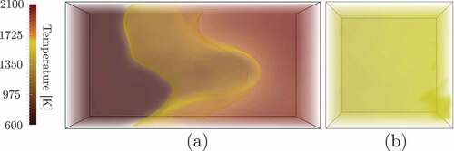
Figure 2 shows the volume rendered temperature field for a conventional premixed combustion case, P1, and the MILD combustion, case AZ1. These figures can be related to digital photographs from experiments showing the variation in luminescence of a flame. The existence of a flame front, and thus strong temperature gradient, in the conventional premixed combustion case is observed. On the other hand, a homogeneous temperature field is observed for the MILD case, which is similar to those observed in photographs from MILD combustion experiments (de Joannon et al., 2000). The volumetrically distributed reaction zones and their frequent interactions result in homogeneous and mild temperature rise resulting in the homogeneous field seen in Figure 2b. This behavior was observed for both premixed (Minamoto et al., 2014b) and non-premixed MILD combustion (Doan et al., 2018). For the premixed case P2, the behavior is similar to the P1 case but with increased wrinkling because of higher turbulence level.

Figure 2. Volume rendered temperature field of (a) conventional turbulent premixed combustion, Case P1, and (b) MILD combustion of Case AZ1.

It is quite common to use OH in experimental studies of turbulent combustion to deduce information on the distribution of HRR in general and this approach has also been used for MILD combustion in past studies. This radical is formed in the flame but it does not go to zero in hot products. Thus, it may become hard to distinguish the OH formed in heat releasing regions from those in the recirculated hot products for MILD combustion. Furthermore, the level of OH formed in the reaction zones may be comparable to or smaller than the background OH level in MILD combustion. These scenarios are assessed carefully in the following discussion. Figure 3 shows the contours of HRR, $Y_{\mathrm{O}\mathrm{H}}$ and $\mathrm{\Delta }{Y}_{\mathrm{O}\mathrm{H}}$ for case AZ1. The typical results are shown for the mid $x$-$y$ plane at $t={\tau }_f$. The HRR is concentrated in thin regions even in non-premixed MILD combustion as has been observed by Minamoto and Swaminathan (2014) for premixed MILD combustion. Also, the heat release or chemical reactions start to occur from the inlet plane because of the radicals present in the incoming mixture as observed in earlier MILD combustion studies. This is physical and one would expect this if a computational boundary cuts through reacting regions.

Figure 3. Contours of (a) heat release rate, (b) $\mathrm{T}\mathrm{C}\mathrm{I}\mathrm{M}\mathrm{\_}\mathrm{A}\mathrm{\_}1610575$ and (c) $\mathrm{\Delta }{Y}_{\mathrm{O}\mathrm{H}}$ in the mid $x$–$y$ plane at $t={\tau }_f$ in case AZ1.

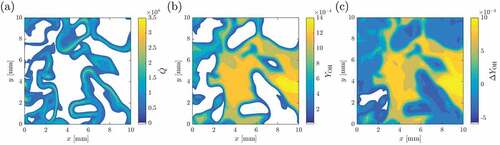
The corresponding spatial variation of OH mass fraction is shown in Figure 3b. The large values of $Y_{\mathrm{O}\mathrm{H}}$ are seen in regions of negligible HRR and these regions contain burnt gases. This is verified by analyzing the relative mass fractions of ${\mathrm{H}}_2\mathrm{O}$, $\mathrm{C}{\mathrm{O}}_2$, etc., which are not shown here. The negligible heat release in these regions can be easily verified by comparing Figure 3a,b. However, if one traces the locations of large $|\mathrm{\nabla }{Y}_{\mathrm{O}\mathrm{H}}|$ then it is quite easy to see that this locus (not shown) follows along the large HRR depicted in Figure 3a and the values of $Y_{\mathrm{O}\mathrm{H}}$ along this locus are nearly 20–30% of its peak value. The LIF imaging of such situation is likely to capture the product gas regions (large OH values) quite vividly and mask the heat releasing locations. Furthermore, these smaller values may not be substantially larger than the background $\mathrm{O}\mathrm{H}$ levels coming from the recirculated exhaust gases. This is verified in Figure 3c by showing the variation of $\mathrm{\Delta }{Y}_{\mathrm{O}\mathrm{H}}=Y_{\mathrm{O}\mathrm{H}}^{\mathrm{R}}-Y_{\mathrm{O}\mathrm{H}}^{\mathrm{C}\mathrm{D}}$. The mass fraction of $\mathrm{O}H$ shown in Figure 3b is denoted by $Y_{\mathrm{O}\mathrm{H}}^{\mathrm{R}}$, and $Y_{\mathrm{O}\mathrm{H}}^{\mathrm{C}\mathrm{D}}$ represents the local $\mathrm{O}\mathrm{H}$ mass fraction value arising from the recirculated hot gases entering through the inlet plane. The latter value is obtained by re-running the case AZ1 but with no reaction and thus there are only convective and diffusive processes. Alternatively, one can conduct another reacting DNS with a passive scalar to represent the incoming OH to obtain $Y_{\mathrm{O}\mathrm{H}}^{\mathrm{C}\mathrm{D}}$. Here, we took the former approach because (i) the reacting DNS was conducted for an earlier study and repeating it is very expensive because of the stiff chemical reactions and (ii) more importantly, the changes in the local velocity between the reactive and non-reactive (convective–diffusive) cases are observed to be very small because the temperature rise from the HRR is only about 150 K. Hence, this approach cannot be used for the conventional combustion cases.

A positive value of $\mathrm{\Delta }{Y}_{\mathrm{O}\mathrm{H}}$ implies that the combustion produced OH is larger than the background value. The negative value implies that (i) the local value is the background value coming from the convective–diffusive processes in regions with no HRR or (ii) $Y_{\mathrm{O}\mathrm{H}}^{\mathrm{C}\mathrm{D}}$ is larger than $Y_{\mathrm{O}\mathrm{H}}^{\mathrm{R}}$ in regions with non-negligible heat release. The second case seems to be paradoxical but it is physical – MILD combustion starts in regions with $\mathrm{\Delta }{Y}_{\mathrm{O}\mathrm{H}}<0$ as has been shown by Doan and Swaminathan (2019) and the production of $\mathrm{O}\mathrm{H}$ in these regions is smaller than the consumption of the background $\mathrm{O}\mathrm{H}$. The values of $\mathrm{\Delta }{Y}_{\mathrm{O}\mathrm{H}}$ is around zero in the locations corresponding to the large HRR (cf. Figure 3a,b). Thus, one needs to be cautious while interpreting $\mathrm{O}\mathrm{H}$-PLIF images to deduce characteristics of reaction zones or to identify heat releasing regions in MILD combustion.

The pdf (probability density function) of $\mathrm{\Delta }{Y}_{\mathrm{O}\mathrm{H}}$ constructed from the DNS data is shown in Figure 4 for the case AZ1. This pdf conditioned on the HRR, $\dot{Q}$, shows that the most probable value of $\mathrm{\Delta }{Y}_{\mathrm{O}\mathrm{H}}$ is about $1\times {10}^{-4}$, which is nearly 1/10th of the most probable largest value observed in the low heat releasing regions. The right peak for the low HRR corresponds to the burnt mixtures while the left peak is for the mixtures beginning to react. This behavior would be similar for the more diluted case BZ1 (not shown). These results point out that LIF imaging for MILD combustion needs more care and closer attention. The commonly employed LIF markers for the heat release are investigated next.

Figure 4. Pdf of $\mathrm{\Delta }{Y}_{\mathrm{O}\mathrm{H}}=Y_{\mathrm{O}\mathrm{H}}^{\mathrm{R}}-Y_{\mathrm{O}\mathrm{H}}^{\mathrm{C}\mathrm{D}}$ from Case AZ1 at $t={\tau }_f$.

Markers for heat release

The chemical markers for heat release used in experiments are based on chemiluminescence or LIF of some species. One can deduce the LIF signals using the DNS data and thus it is possible to evaluate the adequacy of these methods by comparing the heat release from the DNS to those obtained using the deduced LIF signals. This has been done in many past studies for premixed combustion (Chi et al., 2018; Minamoto and Swaminathan, 2014; Nikolaou and Swaminathan, 2014; Wabel et al., 2018) and also for premixed MILD combustion (Minamoto and Swaminathan, 2014). However, it is not quite easy to deduce the chemiluminescence signal from DNS unless the chemiluminescent species are transported in the simulations. The current DNS of non-premixed MILD combustion included $\mathrm{O}{\mathrm{H}}^{\ast }$, one of the chemiluminescence species, in the chemical kinetic mechanism and thus this transported $\mathrm{O}{\mathrm{H}}^{\ast }$ can be used.

The PLIF signal, $S_{\alpha }$, of a species $\alpha$ depends on the species molar concentration $[\alpha ]$ and temperature. This dependence is given by

(1) $S_{\alpha }\propto [\alpha ]T^{(1-\beta )}.$(1)

The commonly used species for PLIF are $\mathrm{C}{\mathrm{H}}_2\mathrm{O}$, OH and HCO. The LIF of atomic hydrogen H needs two-photon techniques as has been demonstrated in past studies (Kulatilaka et al., 2009; Marshall and Pitz, 2018; Mulla et al., 2016) and is also analyzed here. The values of $\beta$ for this study is set to be 2.6 for $\mathrm{C}{\mathrm{H}}_2\mathrm{O}$, 0 for OH and 1.25 for $\mathrm{H}\mathrm{C}\mathrm{O}$ based on past experimental studies (Najm et al., 1998; Paul and Najm, 1998). The value of this parameter for the atomic hydrogen is 2 (Kulatilaka et al., 2009). There are, however, some uncertainties for the $\beta$ values but the results did not change unduly if slightly different values are used. As noted in the Introduction, the product of two LIF signals, for example $\left(\mathrm{O}\mathrm{H}\times \mathrm{C}{\mathrm{H}}_2\mathrm{O}\right)$ or $\left(\mathrm{H}\times \mathrm{C}{\mathrm{H}}_2\mathrm{O}\right)$, is also used to mark heat releasing regions in combustion of hydrocarbon-air mixtures. Hence, we shall also consider these two-scalar based markers.

Figure 5 compares the synthesized PLIF signals for various heat release markers. These typical results, extracted using a single snapshot, are shown in the mid $x$–$y$ plane for the case AZ1. All of the quantities shown in the figure are normalized using their respective maximum values in the mid $x$–$y$ plane and these normalized quantities are denoted using a “tilde”. It is observed that the synthesized single species markers of $\mathrm{O}\mathrm{H}$, $\mathrm{C}{\mathrm{H}}_2\mathrm{O}$ and $\mathrm{H}$ do not represent the features of heat release shown in Figure 5a quite well. Indeed, Figure 5b,d depicting the $\mathrm{O}\mathrm{H}$- and $\mathrm{H}$-PLIF signals show that these two species are present in the downstream regions with nearly no reaction and they do not show up in heat releasing regions in the upstream part. This is because $\mathrm{O}\mathrm{H}$ and $\mathrm{H}$ radicals are consumed in the upstream regions where MILD combustion begins (Doan and Swaminathan, 2019). As one moves downstream, these species are found in regions with small heat release as products of combustion. On the other hand, the precursor species $\mathrm{C}{\mathrm{H}}_2\mathrm{O}$ is present in some of the upstream non-reacting regions. Only $\widetilde{S_{\mathrm{H}\mathrm{C}\mathrm{O}}}$ shown in Figure 5e represents the $\tilde{\dot{Q}}$ well. The two-scalar based markers $\tilde{S_{\mathrm{O}\mathrm{H}}\times S_{\mathrm{C}{\mathrm{H}}_2\mathrm{O}}}$ and $\tilde{S_{\mathrm{H}}\times S_{\mathrm{C}{\mathrm{H}}_2\mathrm{O}}}$ also reproduce most features of the heat releasing zones quite well. The PLIF image of $\tilde{S_{\mathrm{H}}\times S_{\mathrm{C}{\mathrm{H}}_2\mathrm{O}}}$ is similar to $\tilde{S_{\mathrm{O}\mathrm{H}}\times S_{\mathrm{C}{\mathrm{H}}_2\mathrm{O}}}$ and so it is not shown here.

Figure 5. Contours of (a) $\tilde{\dot{Q}}$, (b) $\widetilde{S_{\mathrm{O}\mathrm{H}}}$, (c) $\tilde{S_{\mathrm{C}{\mathrm{H}}_2\mathrm{O}}}$, (d) $\widetilde{S_{\mathrm{H}}}$, (e) $\widetilde{S_{\mathrm{H}\mathrm{C}\mathrm{O}}}$ and (f) $\tilde{S_{\mathrm{O}\mathrm{H}}\times S_{\mathrm{C}{\mathrm{H}}_2\mathrm{O}}}$ in the mid $x$–$y$ plane for case AZ1 at $t=1.5{\tau }_f$. Dark to light gray lines are for iso-contours of values 0.1, 0.2, .., 0.9.

The spatial correlation seen in Figure 5 becomes clearer if one cross plots the LIF signal with the HRR since a good marker should have the data points along the diagonal. Figure 6 shows the scatter plot for the case shown in Figure 5. These results do not change unduly if one uses the data from various planes or the entire computational volume or at different time instants. It is clear that the PLIF of $\mathrm{O}\mathrm{H}$, $\mathrm{H}$ and $\mathrm{C}{\mathrm{H}}_2\mathrm{O}$ are inadequate. As discussed earlier, $\widetilde{S_{\mathrm{O}\mathrm{H}}}$ shows a large scatter since it is present in regions of low heat release and it is absent in the upstream heat releasing regions. Although $\tilde{S_{\mathrm{C}{\mathrm{H}}_2\mathrm{O}}}$ is similar to that for $\widetilde{S_{\mathrm{O}\mathrm{H}}}$, it behaves differently. It is overly present in the upstream regions just ahead of heat releasing regions and absent in downstream regions as one would expect for a precursor. This is consistent with the findings of Medwell et al. (2009) where both $\mathrm{O}\mathrm{H}$ and $\mathrm{C}{\mathrm{H}}_2\mathrm{O}$ were exhibiting different behaviors than in conventional combustion, which led to reaction weakening in MILD combustion. The atomic hydrogen $\mathrm{H}$ behaves somewhat similar to $\mathrm{O}\mathrm{H}$ (see Figure 5b,d also). Figure 6e,f depict that the $\widetilde{S_{\mathrm{H}\mathrm{C}\mathrm{O}}}$ and the two-scalar marker $\left(\tilde{S_{\mathrm{O}\mathrm{H}}\times S_{\mathrm{C}{\mathrm{H}}_2\mathrm{O}}}\right)$ are good. The marker $\left(\tilde{S_{\mathrm{H}}\times S_{\mathrm{C}{\mathrm{H}}_2\mathrm{O}}}\right)$ behaves very similar to $\left(\tilde{S_{\mathrm{O}\mathrm{H}}\times S_{\mathrm{C}{\mathrm{H}}_2\mathrm{O}}}\right)$ and thus it is not shown here. The result of $\widetilde{[\mathrm{O}{\mathrm{H}}^{\ast }]}$ will be discussed later.

Figure 6. Scatter plots of normalized heat release rate vs (a) $\widetilde{[\mathrm{O}{\mathrm{H}}^{\ast }]}$, (b) $\widetilde{S_{\mathrm{O}\mathrm{H}}}$, (c) $\tilde{S_{\mathrm{C}{\mathrm{H}}_2\mathrm{O}}}$, (d) $\widetilde{S_{\mathrm{H}}}$, (e) $\widetilde{S_{\mathrm{H}\mathrm{C}\mathrm{O}}}$ and (f) $\tilde{S_{\mathrm{O}\mathrm{H}}\times S_{\mathrm{C}{\mathrm{H}}_2\mathrm{O}}}$ for case AZ1 obtained using the data shown in Figure 5. Points are colored by their streamwise locations.

The correlation between the various markers and heat release is quantified in Table 4 using the Pearson correlation coefficient. It is observed that $\widetilde{S_{\mathrm{H}\mathrm{C}\mathrm{O}}}$, $\left(\tilde{S_{\mathrm{O}\mathrm{H}}\times S_{\mathrm{C}{\mathrm{H}}_2\mathrm{O}}}\right)$ and $\left(\tilde{S_{\mathrm{H}}\times S_{\mathrm{C}{\mathrm{H}}_2\mathrm{O}}}\right)$ are the only adequate HRR markers since their correlation coefficients are generally larger than 0.9. Although the correlation coefficient for $\widetilde{S_{\mathrm{H}\mathrm{C}\mathrm{O}}}$ is about 0.95 it is generally hard to use this marker because of its low signal-to-noise ratio (Paul and Najm, 1998; Tanahashi et al., 2005) but this has been improved recently using multimode lasers (Kiefer et al., 2009; Zhou et al., 2014). The coefficients for the other cases are also listed in Table 4. Although there is some variations among the cases, the relative merit of various markers noted above for the case AZ1 also holds for other cases. These correlation coefficients do not change if one uses data from another plane or the entire computational volume or multiple snapshots. This is because, the MILD combustion is homogeneous (see Figure 2).

Table 4. Pearson correlation coefficients for the $\tilde{\dot{Q}}$-$\widetilde{S_{\alpha }}$ scatter plots.

Case	$\widetilde{[\mathrm{O}{\mathrm{H}}^{\ast }]}$	$\widetilde{S_{\mathrm{O}\mathrm{H}}}$	$\tilde{S_{\mathrm{C}{\mathrm{H}}_2\mathrm{O}}}$	$\widetilde{S_{\mathrm{H}}}$	$\widetilde{S_{\mathrm{H}\mathrm{C}\mathrm{O}}}$	$\tilde{S_{\mathrm{O}\mathrm{H}}\times S_{\mathrm{C}{\mathrm{H}}_2\mathrm{O}}}$	$\tilde{S_{\mathrm{H}}\times S_{\mathrm{C}{\mathrm{H}}_2\mathrm{O}}}$
AZ1	0.9153	−0.4835	0.5407	−0.1454	0.9447	0.9543	0.9549
AZ2	0.9431	0.0134	0.0890	0.3532	0.9511	0.9557	0.9306
BZ1	0.9458	0.2023	0.1091	0.4009	0.9529	0.9555	0.9279

In addition to the PLIF images discussed above, $\mathrm{O}{\mathrm{H}}^{\ast }$ chemiluminescence signal is also used to identify heat releasing regions. This technique is based on the line-of-sight method implying that the information captured through this signal is averaged along the line of sight. Typically, $\mathrm{C}{\mathrm{H}}^{\ast }$ or $\mathrm{O}{\mathrm{H}}^{\ast }$ is used for this method. In this work, only $\mathrm{O}{\mathrm{H}}^{\ast }$ is considered as it is the only chemiluminescent species available in the chemical mechanism used for the DNS (Doan et al., 2018). The chemiluminescent signal is constructed using Eq. (1) without the temperature dependence employing the transported mole fraction of $\mathrm{O}{\mathrm{H}}^{\ast }$. Figure 7 shows the volume rendered (line-of-sight) images of normalized HRR $\tilde{\dot{Q}}$ and $\widetilde{[\mathrm{O}{\mathrm{H}}^{\ast }]}$ for a qualitative comparison. A reasonably good qualitative agreement between the two images is seen and gross features and locations of the heat releasing regions are captured quite well. However, there are some minor differences. The scatter plot of these two quantities is shown in Figure 6a with the corresponding correlation coefficients listed in Table 4. Although there is some scatter in Figure 6a, the correlation coefficient is larger than 0.9 suggesting that $\mathrm{O}{\mathrm{H}}^{\ast }$ is a good marker to identify heat releasing zones. This is specifically so when compared to OH which has a significantly lower correlation coefficient.

Figure 7. Volume rendered images of normalized (a) heat release rate, $\tilde{\dot{Q}}$, and (b) $\widetilde{[\mathrm{O}{\mathrm{H}}^{\ast }]}$ for the case AZ1.

Premixed or non-premixed mode identification

Hartl et al. (2018) proposed a methodology to distinguish premixed from non-premixed modes in mixed-mode combustion using CEMA of Lu et al. (2010). The Jacobian of the chemical source term with respect to the thermodynamic quantities (temperature, species mole fractions and internal energy) is estimated first in this approach. Then, the eigenvalues of this Jacobian are computed and the eigenvalue with the largest real part, ${\lambda }_e$, is extracted. The $\mathrm{C}\mathrm{M}$ indicator is obtained using this ${\lambda }_e$ as

(2) $\mathrm{C}\mathrm{M}=\mathrm{s}\mathrm{i}\mathrm{g}\mathrm{n}\left(\mathrm{\Re }({\lambda }_e)\right){log}_{10}\left(1+|\mathrm{\Re }({\lambda }_e)|\right)$(2)

where $\mathrm{\Re }({\lambda }_e)$ is the real part of ${\lambda }_e$. A zero crossing of $\mathrm{C}M$ (sign changing from positive to negative) with a near constant mixture fraction value was noted to indicate premixed combustion. A region undergoing non-premixed combustion was characterized by the presence of heat release and $\mathrm{C}\mathrm{M}<0$ with a large variation of mixture fraction. The temperature and major species measured using 1D Raman/Rayleigh measurements and minor species and reaction rates obtained from homogenous reactor calculations constrained by the measured quantities were used to calculate the $\mathrm{C}\mathrm{M}$ indicator by Hartl et al. (2018). However, there is only one component of the local mixture fraction gradient in the 1D measurements along a line. Their study can be consulted for further details.

The DNS data can be used to compute the $\mathrm{C}\mathrm{M}$ indicator directly and compared to the FI analysis. The FI originally proposed by Yamashita et al. (1996) was modified by Briones et al. (2006) to distinguish lean and rich premixed from non-premixed combustion. This FI is given by

(3) $\mathrm{F}\mathrm{I}=\frac{Z-Z_{st}}{2|Z-Z_{st}|}\left(1+\frac{\mathrm{\nabla }{Y}_{\mathrm{C}{\mathrm{H}}_4}\cdot \mathrm{\nabla }{Y}_{{\mathrm{O}}_2}}{|\mathrm{\nabla }{Y}_{\mathrm{C}{\mathrm{H}}_4}||\mathrm{\nabla }{Y}_{{\mathrm{O}}_2}|}\right)$(3)

where $Z_{st}$ is the stoichiometric mixture fraction. The first part of the above equation is simply a “sign” or “signum” function. A zero value of FI indicates a non-premixed mode, while −1 and +1 respectively denote lean and rich premixed modes. The contribution of rich premixed combustion to the total HRR was shown to be smaller than 10% by Doan et al. (2018) for the non-premixed MILD combustion cases used for this study. This is because of the globally lean mixtures used for those DNS cases. The non-premixed mode contribution varied from 11% to 20% for the total HRR depending on the dilution level. Hence, the interest here is on the comparison of non-premixed combustion regions identified using the $\mathrm{C}\mathrm{M}$ and FI indicators. Thus, regions with only $\mathrm{C}\mathrm{M}<0$ will be considered and these region should have $\mathrm{F}\mathrm{I}=0$. This analysis is done only for the non-premixed MILD cases, AZ1, AZ2 and BZ1, since they involve mixture fraction variations.

The variations of FI and CM for case AZ1 in the mid $x$–$y$ plane are shown respectively in Figure 8a,b. These are shown only for regions with the normalized HRR, ${\dot{Q}}^{+}=\dot{Q}{\delta }_{th}/({\rho }_r{s}_L{C}_p(T_b-T_r))$, larger than 1 and the normalizing quantities used are for the local mixture fraction value. The above conditioning on ${\dot{Q}}^{+}$ allows one to focus on regions with significant heat release where the FI and CM indices are meaningful. The results presented here are not unduly influenced by the exact value used for this threshold as long as sufficient number of regions (samples) with significant HRR are identified. The choice of ${\dot{Q}}^{+}\ge 1$ is guided by earlier DNS studies of MILD combustion. It is observed that most of these regions have $\mathrm{C}\mathrm{M}>0$ indicating the presence of strong chemical activities or chemical explosive modes. There is, however, only a small region with $\mathrm{C}\mathrm{M}<0$ which is also marked in Figure 8b. This region is supposed to be a non-premixed region which is also confirmed by the FI results, ie., $\mathrm{F}\mathrm{I}=0$, shown in Figure 8a. There are other regions with negative $\mathrm{C}\mathrm{M}$ but these are indicated to be lean premixed regions by the FI.

Figure 8. Variations of $\mathrm{F}\mathrm{I}$ (in a,c) and $\mathrm{C}\mathrm{M}$ (b,d) in the mid $x$–$y$ plane for cases AZ1 (a,b) and BZ1 (c,d) at $t=1.5{\tau }_f$. The results are shown for regions with ${\dot{Q}}^{+}\ge 1.0$.

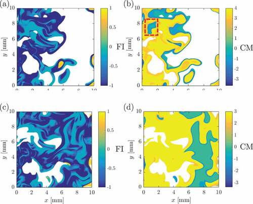
The non-premixed mode contribution was shown to increase with increasing dilution by Doan et al. (2018) and thus it is instructive to see if this trend is captured by the $\mathrm{C}\mathrm{M}$ indicator. The results for the case BZ1 are shown in Figure 8c,d respectively for the $\mathrm{F}\mathrm{I}$ and $\mathrm{C}\mathrm{M}$ indicators. Indeed, there is an increase in the regions with $\mathrm{C}\mathrm{M}<0$ but these regions include those with lean premixed combustion (indicated by $\mathrm{F}\mathrm{I}\simeq -1$). The qualitative comparisons shown in Figure 8 suggest that there is some agreement between $\mathrm{C}\mathrm{M}$ and $\mathrm{F}\mathrm{I}$ indicators but there are large differences. The statistical behavior of these quantities can be obtained by constructing the joint-pdf of $\mathrm{F}\mathrm{I}$ and $\mathrm{C}\mathrm{M}$ subject to the condition of $\mathrm{C}\mathrm{M}<0$ because of the interest here.

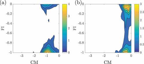
Figure 9 shows the joint-pdf of $\mathrm{F}\mathrm{I}$ and $\mathrm{C}\mathrm{M}$ subject to the condition $\mathrm{C}\mathrm{M}<0$ constructed using the samples collected from regions with ${\dot{Q}}^{+}\ge 1$ for both cases AZ1 and BZ1. The above two conditionings ensure that the identified reacting regions are non-premixed as per the views of Hartl et al. (2018). Thus, if the identified regions are indeed non-premixed then one would expect the joint-pdf contours to lie along $\mathrm{F}\mathrm{I}=0$ for all negative values of $\mathrm{C}\mathrm{M}$. The $\mathrm{C}\mathrm{M}$ approach does capture some of the non-premixed regions shown by the upper peak of the pdf and it also includes some lean premixed regions (lower peak). The second aspect comes from the inability to discriminate between a large patch of negative $\mathrm{C}\mathrm{M}$ and the regions of negative $\mathrm{C}\mathrm{M}$ around its zero crossings. The increased contribution of non-premixed mode with higher dilution is also seen in the joint-pdf for the case BZ1 shown in Figure 9b, which is also captured by the $\mathrm{C}\mathrm{M}$ marker. The joint-pdf constructed using samples, subject to the above two conditions, collected over the entire computational volume and the sampling period is similar to that shown in the figure above. Also, similar behavior is observed for the case AZ2 and thus it is not shown here.

Figure 9. Joint-pdf of ($\mathrm{C}\mathrm{M}$, $\mathrm{F}\mathrm{I}$) in regions with ${\dot{Q}}^{+}\ge 1.0$ and $\mathrm{C}\mathrm{M}<0$ for cases (a) AZ1 and (b) BZ1 using samples collected in the mid $x$–$y$ plane at $t=1.5{\tau }_f$ shown in Figure 8.

The above comparison showed that the approach using the $\mathrm{C}\mathrm{M}$ indicator captures the existence of non-premixed mode to some extent. However, it focuses only on identifying regions of negative $\mathrm{C}\mathrm{M}$ and does not distinguish the regions of negative $\mathrm{C}\mathrm{M}$ associated with the zero crossing of $\mathrm{C}\mathrm{M}$ (related to premixed combustion). Hence, the comparison did not distinguish lean premixed and non-premixed modes with CEMA while the FI approach did. Thus, further analysis is needed for this comparison using DNS and experimental data of turbulent partially premixed combustion under conventional and MILD conditions.

Schlieren approach

The next question that we like to tackle briefly is, how to appropriately discriminate the conventional from MILD combustion. This is quite hard to do using OH-LIF for the reasons discussed earlier. Indeed, direct photographs in furnace-like configuration showed no flame but some similarity with conventional flames were shown for MILD combustion in a JHC configuration as pointed out in the Introduction. Despite these, one of the main features reported for MILD combustion is the existence of mild gradients of temperature in experimental (Ozdemir and Peters, 2001; Wünning and Wünning, 1997) and DNS (Minamoto and Swaminathan, 2014) studies. The mild temperature gradient implies mild density gradient as well which is contrasting to a conventional flame having strong density and temperature gradients. Thus, the schlieren method which employs density gradients can be the first step to assess whether the combustion is MILD or not.

A numerical schlieren image can be synthesized using the DNS data by computing (Hadjadj and Kudryavtsev, 2005):

(4) $Sc=\beta exp\left(\frac{-\kappa |\mathrm{\nabla }\rho |}{|\mathrm{\nabla }\rho {|}_{max}}\right)$(4)

with $\beta =0.8$ and $\kappa =15$. These are standard values used for numerical schlieren images and it was observed that the results discussed here are not sensitive to these specific values. Figure 10 shows the schlieren images obtained for the premixed flames (P1 and P2), premixed MILD combustion (P3) and the three non-premixed MILD combustion cases (see Tables 2 and 3). The technique is a line of sight method and thus the images shown has $Sc$ from Eq. (4) integrated along the axis ($z$) normal to the images shown. The values given above for $\beta$ and $\kappa$ are used for all the cases shown in this figure and all the images are generated using the same greyscale so that they can be compared directly. Darker regions mark stronger density gradients, which is the preheat zone in conventional premixed flames, and brighter regions imply almost uniform density field (unreacted and burnt mixtures in premixed flames). The density gradient is almost negligible in reaction zones and thus it will be hard to identify distinctly in the schlieren image. Also, this is a line of sight technique and thus finer details such as flame wrinkling, etc., cannot be gathered from the schlieren images. However, the premixed combustion in flamelets and other regimes such as thin reaction zones or distributed flamelets can be distinguished quite easily. For example, the darker regions of the schlieren image will be thicker for the thin reaction zones combustion regime because the preheat zone with large density gradients is thickened by the small scale turbulence. This feature is seen for the premixed case P2 shown in Figure 10b compared to the case P1 in Figure 10a. The thickening of the preheat zone in thin reaction zones combustion can be seen clearly if a 2D cut of the DNS data is used to construct the numerical schlieren image and this is shown in Figure 11. It is quite obvious that the reaction zones marked using the iso-line of normalized HRR are thin and they are at the back end of the flame.

Figure 10. Numerical schlieren for the premixed cases (a) P1 and (b) P2, (c) premixed MILD combustion case P3 and the non-premixed MILD combustion cases (d) AZ1, (e) AZ2 and (f) BZ1. Axes for cases P1 and P2 are normalized by their respective laminar flame thicknesses.

Figure 11. Numerical schlieren image for the data in the mid $x$–$y$ plane of the (a) MILD combustion case AZ1 and (b) premixed combustion case P2. The iso-lines show the normalized heat release rate (white dotted line is for 0.2, dashed line is for 0.5, dash-dotted line is for 0.7 and solid line is for 0.9).

The schlieren image for the premixed MILD combustion case is shown in Figure 10c and for the non-premixed MILD combustion cases in Figure. 10d–f These images are distinctly different from those for the premixed cases. The density gradients are distributed over a larger region and this gradient comes from flames, ignition fronts and mixing layers of hot products and cooler reactants. It is not straightforward to identify these three elements contributing to the density gradient. However, it is quite straightforward to distinguish MILD combustion from the conventional flames using the images such as those shown in Figure 10. The mixing layers can be distinguished from the heat releasing regions by plotting iso-lines of normalized HRR in a representative plane as shown in Figure 11a for the non-premixed MILD combustion case AZ1. The schlieren image shown in this figure is also constructed using the density gradient in that representative plane. The darker regions with no HRR correspond to the mixing layers. These kinds of information is helpful to delineate MILD combustion from conventional flames. However, obtaining the kind of 2D information shown in Figure 11 using schlieren in experimental studies may not be possible because the schlieren technique is a line of sight method and thus laser diagnostics are very much required to acquire finer information. Nevertheless, schlieren images help to quickly differentiate between MILD and conventional combustion and to establish that the conditions are indeed MILD before applying detailed laser diagnostics.

Conclusions

DNS data of turbulent premixed flames, premixed and non-premixed MILD combustion have been used to analyze the various markers employed to identify heat releasing, premixed and non-premixed reactions zones. For the heat release markers, several choices used quite commonly in experimental studies of turbulent combustion were assessed for their suitability for MILD combustion by synthesizing the laser-induced fluorescence (LIF) signals of these markers using the DNS data. Out of the various single-scalar heat release markers investigated, $\mathrm{H}\mathrm{C}\mathrm{O}$ was observed to be good but it has a poor signal-to-noise ratio which can be improved using multimode lasers (Kiefer et al., 2009; Zhou et al., 2014).The two-scalar markers $\left(\mathrm{O}\mathrm{H}\times \mathrm{C}{\mathrm{H}}_2\mathrm{O}\right)$ and $\left(\mathrm{H}\times \mathrm{C}{\mathrm{H}}_2\mathrm{O}\right)$ were observed to identify the heat releasing zones well in combustion under both premixed and non-premixed MILD conditions. Since the recirculated hot gases in MILD combustion contain many of the single-scalar markers such as $\mathrm{O}\mathrm{H}$, one needs to be cautious in using them. The analysis of the DNS data showed that the local increase in the $\mathrm{O}\mathrm{H}$ values above the background level is very small in regions of large HRR in MILD combustion and thus the commonly used $\mathrm{O}\mathrm{H}$-PLIF may not identify these regions of importance unambiguously. Hence, the heat releasing zone information deduced using $\mathrm{O}\mathrm{H}$-PLIF in MILD combustion must be used cautiously.

The chemiluminescent images based on $\mathrm{O}{\mathrm{H}}^{\ast }$ obtained from the DNS data show a good correlation with heat releasing regions. However, these images are line-of-sight images and thus the finer information on the reaction zones such as their wrinkling, morphology and topology cannot be deduced. Nonetheless, the $\mathrm{O}{\mathrm{H}}^{\ast }$ images allow for an improved identification of reaction zones compared to OH-PLIF for MILD combustion.

The non-premixed MILD combustion was shown to have premixed and non-premixed reaction zones along with autoignition (Doan et al., 2018). Hartl et al. (2018) proposed a methodology using the CEMA concept to distinguish the premixed and non-premixed modes of combustion. This methodology is assessed along with the FI using the DNS data. A comparison with the FI approach shows that the CEMA methodology identifies major parts of the non-premixed regions as premixed. Further work is required to delineate these regions and auto-ignition unambiguously.

The schlieren images deduced using the DNS data clearly identified the differences between the conventional and MILD combustion qualitatively. The images from MILD combustion are characterized by mild gradients of temperature and density. Hence, schlieren imaging can be used to assess quickly whether a combustor is operating under MILD conditions or not before applying detailed laser diagnostics.

It should be noted that none of the methods discussed above helps to distinguish ignition from propagating flames since both are present in MILD combustion. Indeed, the interplay and importance of these two modes in MILD combustion were shown in past studies (Doan and Swaminathan, 2019; Minamoto et al., 2014a) and thus, identifying a marker to distinguish them would allow for additional understanding of MILD combustion. Furthermore, some variations in the suitability of each marker for non-premixed MILD combustion is observed, depending on the dilution level, and analyzing the causes behind these differences would also be of interest. This will be explored in future investigations.

Acknowledgments

N.A.K.D. acknowledges the financial support of the Qualcomm European Research Studentship Fund in Technology. This work used the ARCHER UK National Supercomputing Service (http://www.archer.ac.uk) using the computing time provided by EPSRC under the RAP project numbered e419 and the UKCTRF (e305).

Additional information

Funding

This work was supported by the Qualcomm European Research Studentship Fund in Technology  at the University of Cambridge.

References

- Balachandran, R., Ayoola, B.O., Kaminski, C.F., Dowling, A.P., and Mastorakos, E. 2005. Experimental investigation of the nonlinear response of turbulent premixed flames to imposed inlet velocity oscillations. Combust. Flame, 143(1–2), 37–55. doi:10.1016/j.combustflame.2005.04.009
- Bilger, R.W., Starner, S.H., and Kee, R.J. 1990. On reduced mechanisms for methane-air combustion in nonpremixed flames. Combust. Flame, 80, 135–149. doi:10.1016/0010-2180(90)90122-8
- Briones, A.M., Aggarwal, S.K., and Katta, V.R. 2006. A numerical investigation of flame liftoff, stabilization, and blowout. Phys. Fluids, 18, 043603. doi:10.1063/1.2191851
- Cavaliere, A., and de Joannon, M. 2004. Mild Combustion. Prog. Energy Combust. Sci., 30(4), 329–366. doi:10.1016/j.pecs.2004.02.003
- Chi, C., Janiga, G., Zähringer, K., and Thévenin, D. 2018. DNS study of the optimal heat release rate marker in premixed methane flames. Proc. Combust. Inst., 37(2), 2363–2371. doi:10.1016/j.proci.2018.07.095
- Dally, B.B., Riesmeier, E., and Peters, N. 2004. Effect of fuel mixture on moderate and intense low oxygen dilution combustion. Combust. Flame, 137(4), 418–431. doi:10.1016/j.combustflame.2004.02.011
- de Joannon, M., Saponaro, A., and Cavaliere, A. 2000. Zero-dimensional analysis of diluted oxidation of methane in rich conditions. Proc. Combust. Inst., 28(2), 1639–1646. doi:10.1016/S0082-0784(00)80562-7
- Doan, N.A.K. 2018 Physical Insights of Non-Premixed MILD Combustion using DNS. PhD thesis, University of Cambridge.
- Doan, N.A.K., and Swaminathan, N. 2019. Role of radicals on MILD combustion inception. Proc. Combust. Inst., 37, 4539–4546. doi:10.1016/j.proci.2018.07.038
- Doan, N.A.K., Swaminathan, N., and Minamoto, Y. 2018. DNS of MILD combustion with mixture fraction variations. Combust. Flame, 189, 173–189. doi:10.1016/j.combustflame.2017.10.030
- Duwig, C., Li, B., Li, Z.S., and Aldén, M. 2012. High resolution imaging of flameless and distributed turbulent combustion. Combust. Flame, 159(1), 306–316. doi:10.1016/j.combustflame.2011.06.018
- Fayoux, A., Zähringer, K., Gicquel, O., and Rolon, J.C. 2005. Experimental and numerical determination of heat release in counterflow premixed laminar flames. Proc. Combust. Inst., 30(1), 251–257. doi:10.1016/j.proci.2004.08.210
- Gao, Y., Chakraborty, N., and Swaminathan, N. 2014. Algebraic closure of scalar dissipation rate for large eddy simulations of turbulent premixed combustion. Combust. Sci. Technol., 186(10–11), 1309–1337. doi:10.1080/00102202.2014.934581
- Hadjadj, A., and Kudryavtsev, A. 2005. Computation and flow visualization in high-speed aerodynamics. J. Turbul., 6(16), 1–25. https://doi.org/10.1080/14685240500209775.
- Hartl, S., Geyer, D., Dreizler, A., Magnotti, G., Barlow, R.S., and Hasse, C. 2018. Regime identification from Raman/Rayleigh line measurements in partially premixed flames. Combust. Flame, 189, 126–141. doi:10.1016/j.combustflame.2017.10.024
- Kathrotia, T., Riedel, U., Seipel, A., Moshammer, K., and Brockhinke, A. 2012. Experimental and numerical study of chemiluminescent species in low-pressure flames. Appl. Phys. B Lasers Opt., 107(3), 571–584. doi:10.1007/s00340-012-5002-0
- Katsuki, M., and Hasegawa, T. 1998. The science and technology of combustion in highly preheated air. 27th Symp. Combust., 27, 3135–3146. doi:10.1016/S0082-0784(98)80176-8
- Kiefer, J., Li, Z.S., Seeger, T., Leipertz, A., and Aldén, M. 2009. Planar laser-induced fluorescence of HCO for instantaneous flame front imaging in hydrocarbon flames. Proc. Combust. Inst., 32(1), 921–928. doi:10.1016/j.proci.2008.05.013
- Kulatilaka, W.D., Frank, J.H., and Settersten, T.B. 2009. Interference-free two-photon LIF imaging of atomic hydrogen in flames using picosecond excitation. Proc. Combust. Inst., 32, 955–962. doi:10.1016/j.proci.2008.06.125
- Li, Z.S., Li, B., Sun, Z.W., Bai, X.S., and Aldén, M. 2010. Turbulence and combustion interaction: high resolution local flame front structure visualization using simultaneous single-shot PLIF imaging of CH, OH, and CH2O in a piloted premixed jet flame. Combust. Flame, 157(6), 1087–1096. doi:10.1016/j.combustflame.2010.02.017
- Lu, T.F., Yoo, C.S., Chen, J.H., and Law, C.K. 2010. Three-dimensional direct numerical simulation of a turbulent lifted hydrogen jet flame in heated coflow: a chemical explosive mode analysis. J. Fluid Mech., 652, 45–64. doi:10.1017/S002211201000039X
- Marshall, G., and Pitz, R.W. 2018. Evaluation of heat release indicators in lean premixed H2/air cellular tubular flames. Proc. Combust. Inst., 37(2), 2029–2036.
- Medwell, P.R., Kalt, P.A.M., and Dally, B.B. 2007. Simultaneous imaging of OH, formaldehyde, and temperature of turbulent nonpremixed jet flames in a heated and diluted coflow. Combust. Flame, 148(1–2), 48–61. doi:10.1016/j.combustflame.2006.10.002
- Medwell, P.R., Kalt, P.A.M., and Dally, B.B. 2009. Reaction zone weakening effects under hot and diluted oxidant stream conditions. Combust. Sci. Technol., 181(7), 937–953. doi:10.1080/00102200902904138
- Menon, S. 2018. Multi-scale subgrid modelling of turbulent premixed combustion at engine relevant conditions. Combust. Sci. Technol, Special issue on UKCTRF Workshop 2018.
- Minamoto, Y., and Swaminathan, N. 2014. Scalar gradient behaviour in MILD combustion. Combust. Flame, 161(4), 1063–1075. doi:10.1016/j.combustflame.2013.10.005
- Minamoto, Y., Swaminathan, N., Cant, R.S., and Leung, T. 2014a. a Morphological and statistical features of reaction zones in MILD and premixed combustion. Combust. Flame, 161(11), 2801–2814. doi:10.1016/j.combustflame.2014.04.018
- Minamoto, Y., Swaminathan, N., Cant, R.S., and Leung, T. 2014b. Reaction zones and their structure in MILD Combustion. Combust. Sci. Technol., 186(8), 1075–1096. doi:10.1080/00102202.2014.902814
- Mulla, I.A., Dowlut, A., Hussain, T., Nikolaou, Z.M., Chakravarthy, S.R., Swaminathan, N., and Balachandran, R. 2016. Heat release rate estimation in laminar premixed flames using laser-induced fluorescence of CH2O and H-atom. Combust. Flame, 165, 373–383. doi:10.1016/j.combustflame.2015.12.023
- Najm, H.N., Paul, P.H., Mueller, C.J., and Wyckoff, P.S. 1998. On the adequacy of certain experimental observables as measurements of flame burning rate. Combust. Flame, 113(3), 312–332. doi:10.1016/S0010-2180(97)00209-5
- Nguyen, Q.-V., and Paul, P.H. 1996. The time evolution of a vortex-flame interaction observed via planar imaging of CH and OH. 26th Symp. Combust., 26(1), 357–364. doi:10.1016/S0082-0784(96)80236-0
- Nikolaou, Z.M., and Swaminathan, N. 2014. Heat release rate markers for premixed combustion. Combust. Flame, 161(12), 3073–3084. doi:10.1016/j.combustflame.2014.05.019
- Ozdemir, I.B., and Peters, N. 2001. Characteristics of the reaction zone in a combustor operating at mild combustion. Exp. Fluids, 30(6), 683–695. doi:10.1007/s003480000248
- Paul, P.H., and Najm, H.N. 1998. Planar laser-induced fluorescence imaging of flame heat release rate. 27th Symp. Combust., 27(1), 43–50. doi:10.1016/S0082-0784(98)80388-3
- Plessing, T., Peters, N., and Wünning, J.G. 1998. Laseroptical investigation of highly preheated combustion with strong exhaust gas recirculation. 27th Symp. Combust., 27, 3197–3204. doi:10.1016/S0082-0784(98)80183-5
- Pope, S.B. 2013. Small scales, many species and the manifold challenges of turbulent combustion. Proc. Combust. Inst., 34(1), 1–31. doi:10.1016/j.proci.2012.09.009
- Richter, M., Collin, R., Nygren, J., Aldén, M., Hildingsson, L., and Johansson, B. 2005. Studies of the combustion process with simultaneous formaldehyde and OH PLIF in a direct-injected HCCI engine. JSME Int. J. Ser. B, 48(4), 701–707. doi:10.1299/jsmeb.48.701
- Rosell, J., Bai, X.-S., Sjoholm, J., Zhou, B., Li, Z., Wang, Z., Petersson, P., Li, Z., Richter, M., and Aldén, M. 2017. Multi-species PLIF study of the structures of turbulent premixed methane/air jet flames in the flamelet and thin-reaction zones regimes. Combust. Flame, 182, 324–338. doi:10.1016/j.combustflame.2017.04.003
- Sidey, J.A.M., Mastorakos, E., and Gordon, R.L. 2014. Simulations of autoignition and laminar premixed flames in methane/air mixtures diluted with hot products. Combust. Sci. Technol., 186(4–5), 453–465. doi:10.1080/00102202.2014.883217
- Smooke, M.D., and Giovangigli, V. 1991. Formulation of the premixed and nonpremixed test problems. In Reduc. Kinet. Mech. Asymptot. Approx. Methane-Air Flames, (Ed.) Smooke, M.D., Lecture Notes in Physics Vol. 384, pp. 1–28. Berlin/Heidelberg: Springer Berlin Heidelberg.
- Sorrentino, G., Sabia, P., de Joannon, M., Cavaliere, A., and Ragucci, R. 2016. The effect of diluent on the sustainability of MILD combustion in a cyclonic burner. Flow, Turbul. Combust., 96(2), 449–468. doi:10.1007/s10494-015-9668-3
- Tanahashi, M., Murakami, S., Choi, G.-M., Fukuchi, Y., and Miyauchi, T. 2005. Simultaneous CHOH PLIF and stereoscopic PIV measurements of turbulent premixed flames. Proc. Combust. Inst., 30(1), 1665–1672. doi:10.1016/j.proci.2004.08.270
- Wabel, T.M., Zhang, P., Zhao, X., Wang, H., Hawkes, E., and Steinberg, A.M. 2018. Assessment of chemical scalars for heat release rate measurement in highly turbulent premixed combustion including experimental factors. Combust. Flame, 194, 485–506. doi:10.1016/j.combustflame.2018.04.016
- Wünning, J.A., and Wünning, J.G. 1997. Flameless oxidation to reduce thermal no-formation. Prog. Energy Combust. Sci., 23(1), 81–94. doi:10.1016/S0360-1285(97)00006-3
- Yamashita, H., Shimada, M., and Takeno, T. 1996. A numerical study on flame stability at the transition point of jet diffusion flames. 26th Symp. Combust., 26(1), 27–34. doi:10.1016/S0082-0784(96)80196-2
- Zhou, B., Kiefer, J., Zetterberg, J., Li, Z., and Aldén, M. 2014. Strategy for PLIF single-shot HCO imaging in turbulent methane/air flames. Combust. Flame, 161, 1566–1574. doi:10.1016/j.combustflame.2013.11.019