Restoring Property of the Michelson–Sivashinsky Equation

ABSTRACT

In this paper, we propose a derivation of the Michelson–Sivashinsky (MS) equation that is based on front propagation only, in opposition to the classical derivation based also on the flow field. Hence, the characteristics of the flow field are here reflected into the characteristics of the fluctuations of the front positions. As a consequence of the presence of the nonlocal term in the MS equation, the probability distribution of the fluctuations of the front positions results to be a quasi-probability distribution, i.e. a density function with negative values. We discuss that the appearance of these negative values, and so the failure of the pure diffusive approach that we adopted is mainly due to a restoring property that is inherent to the phenomenology of the MS equation. We suggest to use these negative values to model local extinction and counter-gradient phenomena.

KEYWORDS:

• Turbulent premixed combustion
• Michelson–Sivashinsky equation
• G-equation
• fluctuations

In this Short Communication, we focus on the hydrodynamic instabilities in turbulent-premixed combustion that are described by the Michelson–Sivashinsky (MS) equation (Fogla 2010; Michelson and Sivashinsky 1977; Sivashinsky 1977). In particular, we test the feasibility of a derivation of the MS equation that is based on front propagation only, in opposition to the classical derivation based also on the flow field. Hence, the characteristics of the flow field are here reflected into the characteristics of the fluctuations of the front positions. In particular, the nonlocal term in the MS equation, that from classical derivation emerges in relation with the flow velocity at the interface, now explicitly emerges in the evolution equation of the probability density function (PDF) of the fluctuations of the front positions.

By studying the information entropy of the PDF of the fluctuations of front position and its rate, it emerges that the MS equation describes a dynamic that includes the restoring of the system condition. Hence, the fluctuations of the front position are not driven by a diffusive motion only, but also and more by a wave-like motion. This wave-like motion restores the system configuration. This restoring property, that is related to the nonlocal term, is responsible for negative values of the PDF of front position fluctuations and highlights that a pure diffusive model is not consistent with the dynamics of the MS equation. Notwithstanding this, we propose such negative values as a mere ad hoc modeling approach for local extinction and counter-gradient phenomena. The discussed derivation can be understood also as an alternative method for computing the solution of MS equation that provides properties that are complementary to, for example, the skewness of the flame curvature (Creta et al. 2016; Zhang et al. 2019) or the stability of the front (Assier and Wu 2014; Vaynblat and Matalon 2000a, 2000b).

The one-dimensional MS equation is

(1) $\frac{\mathrm{\partial }\varphi }{\mathrm{\partial }t}=\frac{{\mathrm{\partial }}^2\varphi }{\mathrm{\partial }{x}^2}-{\left(\frac{\mathrm{\partial }\varphi }{\mathrm{\partial }x}\right)}^2-{\mathbb{D}}_x^1\varphi ,$(1)

where ${\mathbb{D}}_x^1$ is the nonlocal space-fractional derivative in the sense of Riesz–Feller (Podlubny 1999) of order $1$. According to the standard derivation of MS equation in cylindrical symmetry (Fogla 2010), function $\varphi (x)$ represents the height of the flame in point $x$ of the axis directed along the size of the cylinder. Hence, in MS equation the space derivative and the nonlocality refers to “neighbor” points belonging to the flame plane. The main idea here is to replace these tangential “neighboring” effects into random effects, namely $\varphi (x)$ is still the height of the flame with respect to a reference located in $x$ but such height is modeled as the average position of a random front fluctuating with respect to a reference front, and these fluctuations are from a tangential plane.

In analogy with a previous modeling approach (Pagnini and Bonomi 2011), we introduce the field $g(\mathit{y},t)$ defined by

(2) $g(\mathit{y},t)={\int }_{\stackrel{⌣}{\mathrm{\Omega }}(t)}{\mathcal{P}}_c(\mathit{y}-\hat{\mathit{y}};t)d\hat{\mathit{y}},$(2)

where $\stackrel{⌣}{\mathrm{\Omega }}(t)$ is the domain enclosed by the front contour provided by the G-equation for the mean front position (Oberlack, Wenzel, Peters 2001)

(3) $\frac{\mathrm{\partial }\stackrel{⌣}{G}}{\mathrm{\partial }t}+\hat{\mathit{u}}\cdot \mathrm{\nabla }\stackrel{⌣}{G}=s_T\parallel \mathrm{\nabla }\stackrel{⌣}{G}\parallel ,$(3)

where $s_T$ is the turbulent burning velocity, and ${\mathcal{P}}_c(\mathit{x};t)$ is the PDF of the fluctuations of the front positions.

Let any point $x$ of equation (1) be the point of tangency of an iso-line of $g(\mathit{y},t)$ such that all these points of tangency $x$ form both the space-axis in equation (1) and also the whole envelope of a family of reference fronts (in analogy with Huygen’s principle): this family is the consequence of the evolution of an ensemble of source points.

The fluctuations of the positions of the random front are in the tangential direction with respect to the reference front $\stackrel{⌣}{G}$, then we look for an evolution equation for the PDF of front fluctuations in this direction only, such that it reduces to a one-dimensional problem along an axis that we call $r$. Consider the fractional differential equation

(4) $\frac{\mathrm{\partial }{\mathcal{P}}_c}{\mathrm{\partial }t}=\frac{{\mathrm{\partial }}^2{\mathcal{P}}_c}{\mathrm{\partial }{r}^2}-{\mathbb{D}}_r^1{\mathcal{P}}_c,{\mathcal{P}}_c(r;0)=\delta (r),$(4)

then, its solution can be written in integral form as follows

(5) ${\mathcal{P}}_c(r,t)=\frac{1}{2\pi }{\int }_{-\mathrm{\infty }}^{+\mathrm{\infty }}{\mathrm{e}}^{-i\xi r}{\mathrm{e}}^{-{\xi }^{2}t+|\xi |t}d\xi .$(5)

The second term on the RHS of (4), because of the sign minus, may be understood as a counter-damping effect of an harmonic oscillator.

Finally, since the fluctuations of the positions of the random front are in the tangential direction with respect to the reference front $\stackrel{⌣}{G}$, and it holds $\mathrm{\nabla }{\mathcal{P}}_c\cdot \mathrm{\nabla }\stackrel{⌣}{G}=0$, under the assumptions of null-mean velocity field, i.e. $\hat{\mathit{u}}=0$, the evolution equation of $g(\mathit{y},t)$ along the tangential axis $r$ is

(6) $\frac{\mathrm{\partial }g}{\mathrm{\partial }t}=\frac{{\mathrm{\partial }}^{2}g}{\mathrm{\partial }{r}^2}-{\mathbb{D}}_r^{1}g+{\int }_{\stackrel{⌣}{\mathcal{L}}(t)}{s}_T(\hat{r},t){\mathcal{P}}_c(r-\hat{r};t)d\hat{r},$(6)

where $\stackrel{⌣}{\mathcal{L}}(t)$ is the size of a section of the domain $\stackrel{⌣}{\mathrm{\Omega }}(t)$ aligned with the tangential axis $r$. Let $s_T^{\ast }(\hat{\mathit{y}},t)=s_T(\hat{\mathit{y}},t)\mathrm{\nabla }\cdot \hat{\mathit{n}}$, with $\hat{\mathit{n}}=\mathrm{\nabla }\stackrel{⌣}{G}/\parallel \mathrm{\nabla }\stackrel{⌣}{G}\parallel$, then by comparing (1) and (6) we set

(7) $-{\left(\frac{\mathrm{\partial }g}{\mathrm{\partial }r}\right)}^2={\int }_{\stackrel{⌣}{\mathcal{L}}(t)}{s}_T^{\ast }(\hat{r},t){\mathcal{P}}_c(r-\hat{r};t)d\hat{r}\equiv \omega ,$(7)

and $s_T^{\ast }$ turns out to be

(8) $s_T^{\ast }(r,t)=\frac{1}{2\pi }{\int }_{-\mathrm{\infty }}^{+\mathrm{\infty }}{\mathrm{e}}^{-i\xi r}{\mathrm{e}}^{{\xi }^{2}t-|\xi |t}\tilde{\omega }(\xi ,t)d\xi .$(8)

Hence, for any given point $x$, the solution $\varphi (x,t)$ to the MS equation (1) is equal to $g(0,t)$ that can be obtained by computing the integral (2) where the kernel function ${\mathcal{P}}_c$ is the Green function of (4) and $\stackrel{⌣}{G}$ is the solution of the G-equation (3) with $s_T$ established by using (8) for $s_T^{\ast }$.

We stress that the PDF of fluctuations which solves (4) emerges to be a quasi-probability distribution showing negative values that requires high care, see Figures 1 and 2. This fact addresses a non-complete correspondence between the proposed modeling approach for random front propagation and the MS equation. In particular, we argue that this failure is mainly due to a restoring property of the nonlocal term, i.e.

(9) $\frac{1}{2}{\mathbb{D}}_x^1\varphi =\frac{1}{4\pi }{\int }_{-\mathrm{\infty }}^{+\mathrm{\infty }}{\int }_{-\mathrm{\infty }}^{+\mathrm{\infty }}|\xi |{\mathrm{e}}^{i\xi (x-\mu )}\varphi (\mu ,t)d\xi d\mu =v^{\ast },$(9)

Figure 1. Top: evolution in time of the quasi-probability ${\mathcal{P}}_c$ (5). The colors from brown to purple stay for time since $t=0.3$ to $t=18$. Bottom: the same as in the Top panel but for the function $|{\mathcal{P}}_c|$ normalized in order to represent a probability density function.

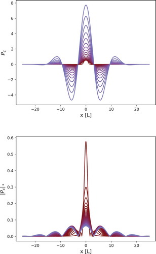
Figure 2. Surface plot of ${\mathcal{P}}_c$. Space is reported in the horizontal axis and time in the vertical axis. The appearance of the two new modes around the $x$-$t$ point $(\pm 10,7)$ establishes a connection with the peak in the information entropy, see Figure 3. We hypothesize that the solution of the considered fractional differential equation (4) due to its nonlocal nature creates new information (two new maximums appear in the quasi Probability ${\mathcal{P}}_c$) thus decreasing the entropy rate of the PDF portrayed in Figure 1.

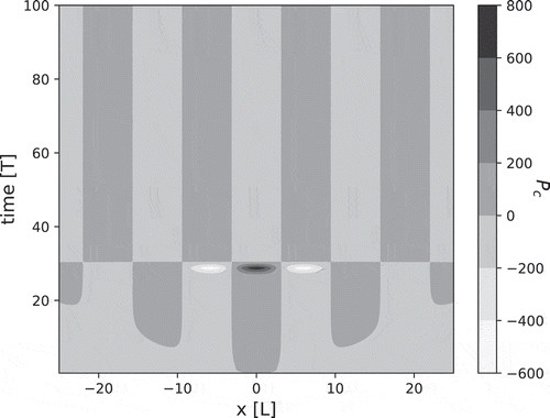
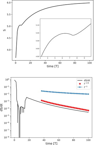
Figure 3. Information entropy (Top) and its rate (Bottom) of the PDF $|{\mathcal{P}}_c|$ versus time. Blue stars and red dots decay as $t^{-1}$ and $t^{-2.6}$, respectively.

where $v^{\ast }$ is the velocity of the flow field at the interface. Then, as a mere modeling approach, the negative values of the quasi-probability can be interpreted as due to local reversibility of the Eulerian progress variable that can be ascribed to the so-called counter-gradient phenomenon. This means that if a fixed point is occupied by a burned volume it turns to be occupied by an unburned one and then the modelization of the local extinction follows, together with the counter-gradient.

To study this restoring we consider the information entropy of the modulus of the PDF ${\mathcal{P}}_c(x;t)$, namely:

(10) $S(t)=-\int |{\mathcal{P}}_c|ln|{\mathcal{P}}_c|dx,$(10)

and the plots of the entropy and the entropy production rate $dS/dt$ are displayed in Figure 3.

The entropy production rate is a measure for the irreversibility of a process. The diffusion equation represents the canonical irreversible process and has positive entropy production. The wave propagation corresponds to the reversible process and has zero entropy production. In Figure 3, we observe that the rate of the information entropy decays faster, i.e. $\sim t^{-2.6}$, than in the standard diffusive case, i.e. $\sim t^{-1}$.

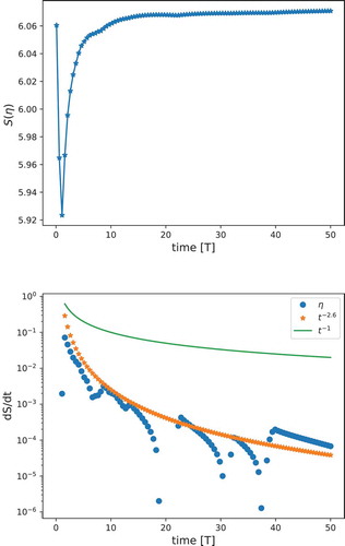
In order to reproduce a similar decay of the rate of information entropy, we look for a simpler equivalent to $|{\mathcal{P}}_c|$ that share similarities with respect to the spatial and temporal variations observed in Figure 2. In particular, we chose a function that expresses temporal and spatial variations in a first window of time, and then decayed to a standing spatial wave depending only on $x$. The selected wave-like function consists of the superposition of a wave and decaying wave-like disturbances with high frequency. In formulas it reads:

(11) $\eta (x,t)=cos\left[\frac{x}{2}\right]+cos[30x]t^{-0.6}.$(11)

In Figure 4, the information entropy and its rate of function $|\eta (x,t)|$ are displayed against the scaling $t^{-1}$ and $t^{-2.6}$, and the fast decay $t^{-2.6}$ is plotted as reference for the entropy. The fact that the same decay of entropy rate of Figure 3 is expressed by making use of a simpler analytical representation confirms that the salient features of the Green function of the fractional differential equation (4) are a spatial (traveling) wave with initial spatiotemporal perturbations.

Figure 4. Information entropy (Top) and its rate (Bottom) of function $|\eta (x,t)|$ defined in (11) versus time. Green line and orange stars decay as $t^{-1}$ and $t^{-2.6}$, respectively.

To conclude, the solution provided by formula (2) highlights through the function ${\mathcal{P}}_c$ the existence of a restoring wave-like motion inside the MS equation. Such behavior cannot be reproduced by a pure diffusive process, and from this the emergence of negative values of ${\mathcal{P}}_c$ and the failure of the proposed approach. This wave-like motion is introduced in the MS equation through the nonlocal velocity $v^{\ast }$ defined in (9). This nonlocal term, together with its sign, provides a restoring force that does not allow for modeling the MS dynamic by diffusive random fronts only (Pagnini and Bonomi 2011).

The emergence of a quasi-probability suggests the idea to introduce, in analogy with quantum mechanics, a probability amplitude whose squared modulus provides the observable for the purely propagating front. In formulas, the following can be stated.

Let $C=|C|{\mathrm{e}}^{iQ}=C_R+i{C}_I$ be a probability amplitude with real and imaginary part. If we assume that function $g(y,t)$ defined in (2), and related to the MS equation (1) as previously derived, corresponds to the square of the real part of $C$, then we have

(12) $g=C_R^2=|C{|}^2-C_I^2,$(12)

where accordingly to definition (2)

(13) $|C{|}^2={\int }_{{\mathcal{P}}_c\ge 0}{\mathcal{P}}_c(x-\hat{x},t)d\hat{x},$(13)

and

(14) $C_I^2=-{\int }_{{\mathcal{P}}_c<0}{\mathcal{P}}_c(x-\hat{x},t)d\hat{x}.$(14)

Hence, the negative values of the quasi-probability result to be associated with the imaginary part of the probability amplitude $C$ and they have a role in slowing the propagation because $C_I^2\ge 0$. In particular, if we integrate (2) in space we have that in correspondence of the negative values of the quasi-probability there is a reduction of the mass amount. Actually, the negative values highlight where statistically the fraction of burned mixture is replaced by unburned mixture.

From this reasoning, we propose to use the negative intervals of the quasi-probability for modeling the non-propagating features of the process as local extinction and counter-gradient phenomena. In fact, the negative values refer to a Eulerian local reversibility of the progress variable (and not to a reversibility of the Lagrangian volume of mixture), that occurs because of the entering of fresh mixture into a volume just now fully burned. This effect can be ascribed first to the local extinction, that stops the propagation of the combustion, and then to the so-called counter-gradient, which is generated by the density difference between reactants and products, that pushes back the front of the burned mixture.

Acknowledgments

The authors would like to acknowledge the editor and the two anonymous referees for their efforts, suggestions and positive attitude that helped us for a proper tailoring of the text which remarkably improved the manuscript.

Additional information

Funding

This work was supported by the Eusko Jaurlaritza [BERC 2014–2017,BERC 2018–2021];Ministerio de Economía y Competitividad [MTM2016-76016-R,SEV-2013-0323,SEV-2017-0718];“la Caixa” Foundation [PhD Grant “La Caixa 2014”].

References

- Assier, R. C., and X. Wu. 2014. Linear and weakly nonlinear instability of a premixed curved flame under the influence of its spontaneous acoustic field. J. Fluid Mech. 758:180–220. doi:10.1017/jfm.2014.525.
- Creta, F., R. Lamioni, P. E. Lapenna, and G. Troiani. 2016. Interplay of Darrieus–Landau instability and weak turbulence in premixed flame propagation. Phys. Rev. E 94:053102. doi:10.1103/PhysRevE.94.053102.
- Fogla, N., Interplay between background turbulence and Darrieus-Landau instability in premixed flames via a model equation. M.S. Thesis at University of Illinois at Urbana-Champaign 2010, http://hdl.handle.net/2142/16182.
- Michelson, D. M., and G. I. Sivashinsky. 1977. Nonlinear analysis of hydrodynamic instability in laminar flames - II. Numerical experiments. Acta Astronaut 4:1207–21. doi:10.1016/0094-5765(77)90097-2.
- Oberlack, M., H. Wenzel, and N. Peters. 2001. On symmetries and averaging of the G-equation for premixed combustion. Combust. Theory Modell. 5:363–83. doi:10.1088/1364-7830/5/3/307.
- Pagnini, G., and E. Bonomi. 2011. Lagrangian formulation of turbulent premixed combustion. Phys. Rev. Lett. 107:044503. doi:10.1103/PhysRevLett.107.044503.
- Podlubny, I. 1999. Fractional differential equations. New York: Academic Press.
- Sivashinsky, G. I. 1977. Nonlinear analysis of hydrodynamic instability in laminar flames - I. Derivation of basic equations. Acta Astronaut 4:1177–206. doi:10.1016/0094-5765(77)90096-0.
- Vaynblat, D., and M. Matalon. 2000a. Stability of pole solutions for planar propagating flames: I. Exact eigenvalues and eigenfunctions. SIAM J. Appl. Math 60:679–702. doi:10.1137/S0036139998346439.
- Vaynblat, D., and M. Matalon. 2000b. Stability of pole solutions for planar propagating flames: II. Properties of eigenvalues/eigenfunctions and implications to stability. SIAM J. Appl. Math 60:703–28. doi:10.1137/S0036139998346440.
- Zhang, M., A. Patyal, Z. Huang, and M. Matalon. 2019. Morphology of wrinkles along the surface of turbulent Bunsen flames – Their amplification and advection due to the Darrieus–Landau instability. Proc. Combust. Inst. 37:2335–43. doi:10.1016/j.proci.2018.06.204.