Characteristic Chemical Time Scales for Reactive Flow Modeling

ABSTRACT

The chemical time scale can be used to characterize a reactive system(’s behavior). In addition, various dimensionless numbers (e.g. Damköhler number) rely on a characteristic chemical time scale. The inverse eigenvalues of a system are regarded as the system’s time scales. This means, the number of time scales is equal the numbers of eigenvalues. A formulation for a single characteristic time scale is required for the system characterization and to calculate dimensionless numbers. Recently proposed modifications of the Eddy Dissipation Concept (a turbulence-chemistry interaction model) also incorporate the Damköhler number in their formulation. Besides accuracy, the numerical efficiency is important, since the chemical time scale needs to be computed in each cell at every time step. We present different chemical time scale definitions found in literature, evaluate them on simple test problems and use them for flame simulations in conjunction with the modified Eddy Dissipation Concept. For the simple test case, most formulations give satisfactory results. The complexity of the chemical reaction mechanism greatly impacts the calculated time scale values. Therefore, we suggest to use a simple global mechanism for the calculation of chemical time scales to ensure reproducibility and consistency of the results.

KEYWORDS:

• Reactive flows
• chemical time scales
• eddy dissipation concept

Introduction

Time scales characterize a system and its behavior. Many dimensionless numbers (e.g. Damköhler, Karlovitz, Stokes number) incorporate time scales and are reported to describe a system(’s behavior) or are used to design scale-up of plants. Many engineering processes incorporate reactive flows. In these cases, it is of particular interest to characterize those flows with time scales.

For reactive flows, the flow itself as well as the reaction determines the overall characteristics. The issue with reaction systems is that their chemical time scale is not inherently defined. Many different time scale definitions or time scale approximations exist in literature. Especially for the calculation of dimensionless numbers a characteristic and representative time scale of the system is needed.

Computational Fluid Dynamics (CFD) can provide detailed information of flows, to determine, for example, flow time scales. But time scale definitions are also used to develop and tailor CFD models. For example, the Eddy Dissipation Concept (EDC) is widely used for the simulation of reactive flows. A recent proposition for its modification incorporates the Damköhler number. This poses the need for a numerically efficient chemical time scale definition to calculate the Damköhler number and apply the suggested modifications in CFD.

Therefore, we discuss the theoretical background of chemical time scales and test proposed definitions for a characteristic chemical time scale, possibly suitable for the application to CFD. These are discussed and applied to simplified test cases, where they can be compared to an analytical solution.

Furthermore, we apply the most suitable chemical time scale formulations to simulations using the modified Eddy Dissipation Concepts and compare them to available flame measurement data. This investigates the practical applicability of the formulations.

Chemical time scales of a system

A chemical reaction system can be described by the following set of Ordinary Differential Equations (ODEs):

(1) $\frac{\mathrm{d}\mathit{Y}}{\mathrm{d}t}=\dot{\mathit{\omega }}\mathrm{w}\mathrm{i}\mathrm{t}\mathrm{h}\mathit{Y}\left(0\right)={\mathit{Y}}_0$(1)

where $\mathit{Y}$ denotes the mass fractions of species and $\dot{\omega }$ denotes the net production/consumption rates. If the system is disturbed with a small perturbation in its initial value (Equation (2)(2) $\mathit{Y}\left(0\right)={\mathit{Y}}_0+\mathrm{\Delta }{\mathit{Y}}_0$(2) ), the change of the ODE can be approximated by the Jacobian $\mathit{J}$ multiplied by $\mathrm{\Delta }\mathit{Y}$ (Equation (3)(3) $\frac{\mathrm{d}\mathrm{\Delta }\mathit{Y}}{\mathrm{d}t}=\mathit{J}\mathrm{\Delta }t$(3) ), see (Nagy and Turànyi 2009; Tomlin, Whitehouse, Pilling 2002).

(2) $\mathit{Y}\left(0\right)={\mathit{Y}}_0+\mathrm{\Delta }{\mathit{Y}}_0$(2)

(3) $\frac{\mathrm{d}\mathrm{\Delta }\mathit{Y}}{\mathrm{d}t}=\mathit{J}\mathrm{\Delta }t$(3)

The Jacobian matrix is defined in the following way and assumed to be independent of time for sufficiently small time intervals:

(4) $\mathit{J}=\frac{\mathrm{\partial }\dot{\mathit{\omega }}}{\mathrm{\partial }\mathit{Y}}$(4)

Therefore, the time evolution of perturbations of the system is assumed to depend on the eigenvalues of the Jacobian, which consequently represent the characteristic time scales of the system. For a more thorough discussion of the connection between time scales and eigenvalues we refer to (Nagy and Turànyi 2009; Tomlin et al. 2002).

For complex reaction mechanisms this leads to large Jacobian matrices and a time scale for each species. These time scales describe the chemical system. In the next section we present formulations to derive one characteristic time scale for chemical reaction systems, which is necessary for the calculation of dimensionless numbers.

Characteristic chemical time scale definitions

Different definitions of the characteristic chemical time scale have been proposed in literature (Caudal et al. 2013; Evans et al. 2019; Golovitchev and Chomiak 2001; Golovitchev and Nordin 2001; Isaac et al. 2013; Lam and Goussis 1991; Li et al. 2017; Løvås et al. 2002; Prüfert et al. 2014; Ren and Goldin 2011). Some of them were derived for the purpose of mechanism reduction and are based on the separation of the chemical system into a slow and a fast reacting subspace to identify the dominating system time scales. Others are based on eigenvalue approximations or simple ones only incorporate the reaction rates.

The main objective for the in-situ application to CFD is to obtain a characteristic chemical time scale which describes the chemical system with sufficient accuracy. The complexity of existing definitions varies greatly from simple algebraic expressions to complex eigenvalue problems or principle component analysis (PCA) (Isaac 2014; Parente et al. 2011). Some of them, for example computational singular perturbation (Lam and Goussis 1991) or intrinsic-low dimensional manifold (Glassmaker 1999), have also been developed for a different purpose and have only been recently adapted to determine a characteristic time scale.

The existing expressions for chemical time scale characterization can be divided into algebraic and eigenvalue based definitions. Typically the algebraic expressions employ combinations of species concentrations, chemical reaction rates and/or species consumption/destruction rates. Eigenvalue based formulations require the calculation or approximation of the Jacobian matrix and its decomposition.

Within this wide variety of definitions, the eigenvalue based, for example the CSP theory, have a solid theoretical foundation, while others try to approximate the characteristic scales of the system. The aim of this study is to identify sufficiently accurate, but numerically efficient, characteristic chemical time scale definitions, which can be applied within CFD. Therefore, selected time scale approximations suitable for in-situ determination from literature are discussed in the following sections. They are compared to an analytical solution of a simple reaction system and are employed within simulations of a “classical” turbulent and a moderate or intense low oxygen dilution (MILD) combustion flame.

Inverse Reaction Rate Time Scale (IRRTS)

The probably simplest time scale definition is the reciprocal of the chemical reaction rate ($k_r$):

(5) ${\tau }_{IRRTS}=\underset{r\in N_R}{min}\left(\frac{1}{\left|k_r\right|}\right)$(5)

where $N_R$ is the number of reactions.

For a global single-step reaction this definition is a good choice, since the chemical time scale is unambiguously defined. However, for more complex mechanisms, as many time scales as reactions exist. In this case, the fastest reaction is assumed to dominate the system, thus, defining the characteristic time scale. A drawback of this approach is that all reactions are considered equally important, although some might be of minor importance due to insignificant educt and/or product concentrations.

Ren Time Scale (RTS)

Ren and Goldin (2011) proposed the minimum ratio of the fuel species mass fraction ($Y_i$) and the corresponding species consumption rates (${\dot{\omega }}_i$) as time scale (Equation (6)(6) ${\tau }_{RTS}=C_e\underset{\genfrac{}{}{0ex}{}{i\in N_s}{{\dot{\omega }}_i<0}}{min}\left(\frac{Y_i}{{\dot{\omega }}_i}\right)$(6) ). Instead of defining a user-defined set of fuel species, in this work all species with a negative net production rate are taken into account. Additionally, Ren and Goldin (2011) introduced an empirical constant $C_e$ to adapt the time scale. Since the numerical value of $C_e$ was not defined, it is set to unity in this work. However, this definition also assumes that the fastest time scale is the dominant one.

(6) ${\tau }_{RTS}=C_e\underset{\genfrac{}{}{0ex}{}{i\in N_s}{{\dot{\omega }}_i<0}}{min}\left(\frac{Y_i}{{\dot{\omega }}_i}\right)$(6)

Ren Product Time Scale (RPTS)

In analogy to RTS, (section 3.2) the Ren Product Time Scale (RPTS) is defined for the product species (Equation (7)(7) ${\tau }_{RPTS}=C_e\underset{\genfrac{}{}{0ex}{}{i\in N_s}{{\dot{\omega }}_i>0}}{min}\left(\frac{Y_i}{{\dot{\omega }}_i}\right)$(7) ). This means all species with a positive net production rate are considered.

(7) ${\tau }_{RPTS}=C_e\underset{\genfrac{}{}{0ex}{}{i\in N_s}{{\dot{\omega }}_i>0}}{min}\left(\frac{Y_i}{{\dot{\omega }}_i}\right)$(7)

OpenFOAM Time Scale (OFTS)

Golovitchev and Nordin (2001) defined the chemical time scale as the ratio of the total species concentration $c_{\mathrm{t}\mathrm{o}\mathrm{t}}$ and the sum of the production rate $k_{f,r}$ times the stoichiometric coefficient $\nu$ of the product species $N_{s,RHS}$. For mechanisms consisting of more than one reaction $n_R$, the ratios of all reactions are summed up, as follows (Li et al. 2018):

(8) ${\tau }_{OFTS}=\sum _{r=1}^{n_R}\frac{c_{\mathrm{t}\mathrm{o}\mathrm{t}}}{{\sum }_{n=1}^{N_{s,RHS}}{\nu }_{n,r}{k}_{f,r}}$(8)

Evans Time Scale (ETS)

Evans et al. (2019) suggests to use the major species $N_{\mathrm{m}\mathrm{a}\mathrm{j}}$ (for example CH₄, H₂, O₂, CO and CO₂) for the time scale definition shown in Equation (9)(9) ${\tau }_{ETS}=\underset{i\in N_{\mathrm{m}\mathrm{a}\mathrm{j}}}{max}\left[\frac{Y_i}{\left|{\dot{\omega }}_i\right|/\rho }\right]$(9) . To avoid using non-reacting species for the calculation, species with a reaction rate ${\dot{\omega }}_i<{10}^{-16}$ are neglected.

(9) ${\tau }_{ETS}=\underset{i\in N_{\mathrm{m}\mathrm{a}\mathrm{j}}}{max}\left[\frac{Y_i}{\left|{\dot{\omega }}_i\right|/\rho }\right]$(9)

Inverse Jacobian Time Scale (IJTS)

The inverse Jacobian time scale requires the numerically expensive calculation of the species rate Jacobian (Equation (4)(4) $\mathit{J}=\frac{\mathrm{\partial }\dot{\mathit{\omega }}}{\mathrm{\partial }\mathit{Y}}$(4) ). Since most chemistry solvers need the Jacobian anyway, the increased numerical effort is negligible. Prüfert et al. (2014) and Caudal et al. (2013) interpreted the diagonal elements of the Jacobian as approximation of the system’s eigenvalues. For diagonal dominant matrices this approximation is valid, see Gerschgorin’s circle theorem (Gerschgorin 1931). However, if the off-diagonal elements are relevant, this approximation can give bad results, since oscillating behavior indicated by complex eigenvalues is not covered. Further information on the quality of the eigenvalue approximation by the Jacobian diagonal can be found elsewhere, e.g. (Prüfert et al. 2014).

One way to get the characteristic time scale is to assume that the inverse of the smallest absolute diagonal element is the dominating time scale (Equation (10)(10) ${\tau }_{IJTS}=min\left(\frac{1}{{\mathcal{J}}_{ii}}\right)$(10) ). However, this approach does not check the significance of the individual time scales.

(10) ${\tau }_{IJTS}=min\left(\frac{1}{{\mathcal{J}}_{ii}}\right)$(10)

Prüfert et al. (2014) defined a relevant sub set of time scales ($i\in \mathcal{I}$) by comparing the sub set reaction rate $\dot{\omega }{e}_i$ and the total absolute rate $\dot{\omega }$ (Equation (11)(11) $∥\left(\sum _{i\in \mathcal{I}}\dot{\omega }{e}_i\right)-\dot{\omega }∥<ϵ$(11) ), where $e_i$ is the i${ }^{th}$ canonical basis vector.

(11) $∥\left(\sum _{i\in \mathcal{I}}\dot{\omega }{e}_i\right)-\dot{\omega }∥<ϵ$(11)

The smallest sub set time scale is then assumed to be the characteristic system time scale.

System Progress Time Scale (SPTS)

Prüfert et al. (2014) also defined a chemical time scale based on the inverse norm of the Jacobian matrix multiplied by a weighting factor. The normalized species consumption rates are employed as weighting factor:

(12) ${\tau }_{SPTS}={\left(∥\mathit{J}\frac{\dot{\mathit{\omega }}\left(t_0\right)}{∥\dot{\mathit{\omega }}\left(t_0\right)∥}∥\right)}^{-1}$(12)

The SPTS represents the time evolution of the whole system, because ${\tau }_{SPTS}$ approximates ${\left|\left|\mathit{J}\right|\right|}^{-1}$. Using the von Mises iteration it can be shown that ${\tau }^{-2}$ converges toward ${\left|\left|\mathit{J}\right|\right|}^2$ (Prüfert et al. 2014). This method incorporates the significance of the different reactions by considering their contribution to the overall progress.

Inverse Eigenvalue Time Scale (IETS)

The simplest eigenvalue based time scale is the Inverse Eigenvalue Time Scale (IETS), which assumes that the largest eigenvalue (${\mathit{\lambda }}_i$) defines the characteristic chemical time scale:

(13) ${\tau }_{IETS}=\underset{i\in N_s}{min}\left(\frac{1}{\left|{\lambda }_i\right|}\right)$(13)

This formulation is also described in (Prüfert et al. 2014) and parts of the derivation are shown in (Caudal et al. 2013; Løvås et al. 2002).

Eigenvalue Time Scale (EVTS)

The Eigenvalue Time Scale (EVTS), also called characteristic time scale identification (CTS-ID) in (Caudal et al. 2013), is based on a complex-to-real transformation of the, in general, complex conjugate eigenvalues and eigenvectors. A transformed matrix $\tilde{V}$ is constructed as:

(14) $\tilde{\mathit{V}}=\left(\begin{array}{cccccc}{L}_1& \hspace{0.17em}& \hspace{0.17em}& \hspace{0.17em}& \hspace{0.17em}& \hspace{0.17em}\\ \hspace{0.17em}& \ddots & \hspace{0.17em}& \hspace{0.17em}& \hspace{0.17em}& \hspace{0.17em}\\ \hspace{0.17em}& \hspace{0.17em}& L_{N_r}& \hspace{0.17em}& \hspace{0.17em}& \hspace{0.17em}\\ \hspace{0.17em}& \hspace{0.17em}& \hspace{0.17em}& {\mathit{L}}_{N_r+1}& \hspace{0.17em}& \hspace{0.17em}\\ \hspace{0.17em}& \hspace{0.17em}& \hspace{0.17em}& \hspace{0.17em}& \ddots & \hspace{0.17em}\\ \hspace{0.17em}& \hspace{0.17em}& \hspace{0.17em}& \hspace{0.17em}& \hspace{0.17em}& {\mathit{L}}_{N_s-1}\end{array}\right)$(14)

with $L_1$ to $L_{N_r}$ being the sorted real eigenvalues and ${\mathit{L}}_{N_r+1}$ to ${\mathit{L}}_{N_s-1}$ being $2\times 2$ block matrices:

(15) ${\mathit{L}}_i=\left[\begin{array}{cc}\mathrm{R}\mathrm{e}\left({\lambda }_i\right)& \mathrm{I}\mathrm{m}\left({\lambda }_i\right)\\ -\mathrm{I}\mathrm{m}\left({\lambda }_i\right)& \mathrm{R}\mathrm{e}\left({\lambda }_i\right)\end{array}\right]$(15)

This matrix describes a transformed system. Then, the system time scales are defined as:

(16) ${\tau }_i=\frac{1}{{\lambda }_i}$(16)

for the real eigenvalues and

(17) ${\tau }_{2i-1+N_r}=\frac{1}{\left|\mathrm{R}\mathrm{e}\left({\lambda }_{2i-1+N_r}\right)\right|}{\tau }_{2i+N_r}=\frac{1}{\left|\mathrm{I}\mathrm{m}\left({\lambda }_{2i-1+N_r}\right)\right|}$(17)

for imaginary eigenvalues. To obtain the important time scales, an importance criterion ${\gamma }_i$ is defined for all species $N_s$ in Equation (18)(18) ${\gamma }_i=\frac{∥a_i{\mathit{b}}_i∥}{{max}_{k\in N_s}∥a_k{\mathit{b}}_k∥}$(18) using the definition in Equation (20)(20) $\mathit{a}={\tilde{\mathit{V}}}^{-1}\dot{\mathit{\omega }}$(20) . In Equation (18)(18) ${\gamma }_i=\frac{∥a_i{\mathit{b}}_i∥}{{max}_{k\in N_s}∥a_k{\mathit{b}}_k∥}$(18) , the transformed vectors ${\mathit{b}}_i$ are used, which originate from the eigenvectors of the original system ${\tilde{\mathit{b}}}_i$. The vectors corresponding to the real eigenvalues ($i=\mathrm{1...}{N}_r$) are equal to the original eigenvectors. The ones corresponding to complex eigenvectors ($i=N_r+\mathrm{1...}{N}_s-1$) are defined in Equation (19)(19) ${\mathit{b}}_{2i-1+N_r}=\mathrm{R}\mathrm{e}\left({\tilde{\mathit{b}}}_{2i-1+N_r}\right){\mathit{b}}_{2i+N_r}=\mathrm{I}\mathrm{m}\left({\tilde{\mathit{b}}}_{2i-1+N_r}\right)$(19) .

(18) ${\gamma }_i=\frac{∥a_i{\mathit{b}}_i∥}{{max}_{k\in N_s}∥a_k{\mathit{b}}_k∥}$(18)

(19) ${\mathit{b}}_{2i-1+N_r}=\mathrm{R}\mathrm{e}\left({\tilde{\mathit{b}}}_{2i-1+N_r}\right){\mathit{b}}_{2i+N_r}=\mathrm{I}\mathrm{m}\left({\tilde{\mathit{b}}}_{2i-1+N_r}\right)$(19)

(20) $\mathit{a}={\tilde{\mathit{V}}}^{-1}\dot{\mathit{\omega }}$(20)

Using the importance criterion ${\gamma }_i$, all time scales greater than a threshold value $ϵ$ are considered to be important. The characteristic chemical time scale of the system is then the smallest of the remaining (important) time scales.

Simple test cases

Single-step reaction

The chemical time scale definitions from section 3 are tested on a simple one-step carbon monoxide (CO) oxidation reaction:

(21) $2\mathrm{C}\mathrm{O}+{\mathrm{O}}_2->2\mathrm{C}{\mathrm{O}}_2$(21)

According to Westbrook and Dryer (1981) the reaction is reversible; the forward rate ($k_f$) depends on the CO, H₂O, and O₂ concentrations (Equation (22)(22) $k_f=\underset{\mathrm{k}}{\underbrace{3.98\cdot {10}^{14}{e}^{-\frac{20129}{T}}}}\left[\mathrm{C}\mathrm{O}\right]{\left[{\mathrm{H}}_2\mathrm{O}\right]}^{0.5}{\left[{\mathrm{O}}_2\right]}^{0.25}$(22) ) while the reverse reaction rate ($k_r$) is a function of the CO₂ concentration (Equation (23)(23) $k_r=5.0\cdot {10}^8{e}^{-\frac{20129}{T}}\left[\mathrm{C}{\mathrm{O}}_2\right]$(23) ). (Units are cm/s/mol/K)

(22) $k_f=\underset{\mathrm{k}}{\underbrace{3.98\cdot {10}^{14}{e}^{-\frac{20129}{T}}}}\left[\mathrm{C}\mathrm{O}\right]{\left[{\mathrm{H}}_2\mathrm{O}\right]}^{0.5}{\left[{\mathrm{O}}_2\right]}^{0.25}$(22)

(23) $k_r=5.0\cdot {10}^8{e}^{-\frac{20129}{T}}\left[\mathrm{C}{\mathrm{O}}_2\right]$(23)

The reverse reaction rate is neglected for this test case. Further simplifying the rate dependency by removing H₂O, a $3\times 3$ matrix is obtained for calculating the eigenvalues of the reaction system:

(24) $\mathrm{d}\mathrm{e}\mathrm{t}\left(\mathcal{J}-\lambda \right)=\left|\left(\begin{array}{ccc}-2k{\left[{\mathrm{O}}_2\right]}^{0.25}-{\lambda }_1& -0.25k\left[\mathrm{C}\mathrm{O}\right]{\left[{\mathrm{O}}_2\right]}^{-0.75}& 0\\ -2k{\left[{\mathrm{O}}_2\right]}^{0.25}& -0.25k\left[\mathrm{C}\mathrm{O}\right]{\left[{\mathrm{O}}_2\right]}^{-0.75}-{\lambda }_2& 0\\ 2k{\left[{\mathrm{O}}_2\right]}^{0.25}& 0.25k\left[\mathrm{C}\mathrm{O}\right]{\left[{\mathrm{O}}_2\right]}^{-0.75}& -{\lambda }_3\end{array}\right)\right|$(24)

The eigenvalues of this matrix can be easily calculated analytically. Only one none zero eigenvalue exists:

(25) ${\lambda }_1=-k{\left[{\mathrm{O}}_2\right]}^{0.25}-0.25k\left[\mathrm{C}\mathrm{O}\right]{\left[{\mathrm{O}}_2\right]}^{-0.75}$(25)

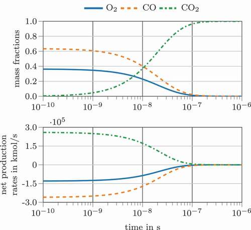
This analytic eigenvalue solution and the resulting chemical time scale is compared to the previously discussed time scale definitions. The conversion of a stoichiometric CO and O₂ mixture at 1500 K and 1 bar is modeled in a plug flow reactor (PFR) with Cantera (Goodwin, Moffat, Speth 2017). Chemical time scales were calculated at each output time step using a threshold value of $ϵ=0.00001$ where necessary. Figure 1 shows the species concentration and the species consumption profiles versus time. Obviously, under these conditions, the CO oxidation is a fast reaction reaching full conversion after around ${10}^{-7}$ seconds.

Figure 1. Species concentration (top) and species rates (bottom) for the simplified, one-step three species carbon monoxide oxidation

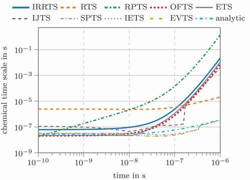
Figure 2 shows the corresponding time scales during the conversion. At the beginning, the different definitions span a range between ${10}^{-8}$ and ${10}^{-7}$ seconds, except for RTS. After around ${10}^{-8}$ second reaction time, different expressions form two groups: one giving a steep decrease in chemical time scales reaching values of more than ${10}^{-3}$ seconds, while the other reaches values around ${10}^{-6}$ seconds, only RTS and RPTS can not clearly be added to those groups. The analytic eigenvalue time scale is part of the latter group. The time scale definitions predicting higher values are the IRRTS, ETS, OFTS and IJTS. One might conclude that the system possesses two distinct time scales. However, since only a single reaction is considered, there should be a clearly defined system time scale. Therefore, the deviations between these two groups can be considered inherent to their definition. A different interpretation could be that the first group represents the current characteristic system velocity, since the time scales increase at a similar rate as the species consumption and production rates (compare Figs. 1 and 2). Contrary, the second group might represent the ability to react on perturbations, meaning that the chemical system compensates disturbances quickly at high temperatures.

Figure 2. Chemical time scales for the simplified, one-step three species carbon monoxide oxidation

Comprehensive reaction mechanism

Comprehensive reaction mechanisms consist of multiple reactions and complex reaction rate dependencies of concentrations and pressure, e.g. Three-Body reactions, SRI, TROE or TSA fall-off (Gilbert et al. 1983; Lindemann et al. 1922; Stewart et al. 1989; Troe 1983; Tsang and Herron 1991). Thus, the calculation of chemical time scales, the Jacobian and eigenvalues becomes numerically more expensive than for an one-step reaction mechanism. Furthermore, identifying the relevant time scales is essential to obtain the characteristic ones. The same initial conditions are employed in combination with the well-known methane combustion mechanism GRI 3.0 (Smith et al. 2018). Figure 3 shows species concentration and species consumption/production rates for the involved main species (CO, CO₂, H₂O, O₂) and radical species (H, O, OH). 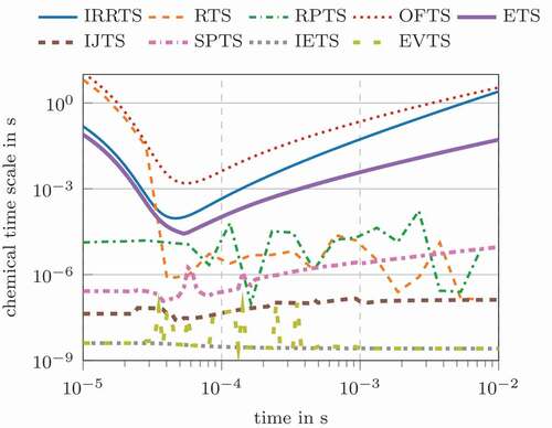The CO oxidation process takes longer when employing the detailed mechanism (${10}^{-3}$ compared to ${10}^{-7}$ seconds). This is caused by an incubation time necessary for the formation of a radical pool which enables the overall oxidation reaction. In this test case, water vapor acts as a reaction promoter, since it forms the radical pool by dissociation. This is clearly visible in the species and consumption rate profiles. However, Figure 4 shows, that not all chemical time scale definitions depict these incubation effects. The IRRTS, ETS and OFTS clearly feature a time scale decrease followed by an increase due to the reaction progress. The SPTS definition indicates a slight decrease, while the IJTS, and IETS predict almost constant chemical time scales around ${10}^{-8}$ seconds. The RTS and RPTS definitions have quite strong fluctuations, caused by the fast changing net production and consumption rates of some radical species.

Figure 3. Species concentration (top) and species rates (bottom) for the carbon monoxide oxidation according to the GRI3.0 mechanism (Smith et al. 2018)

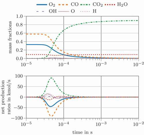
Figure 4. Chemical time scales for the carbon monoxide oxidation based on the GRI3.0 mechanism

Methods for computational fluid dynamics

A characteristic chemical time scale can also be necessary for CFD models. Recently, adaptations of the EDC have been proposed, which need a characteristic chemical time scale (Bao 2017; Parente et al. 2016). Therefore, the EDC is described shortly in the next section and its modifications are discussed.

Eddy dissipation concept

The physical foundation of the EDC is the assumption that educts react only in the fine structures (denoted by $\ast$), since they are mixed on a molecular level there (Magnussen 1981). Based on the turbulent energy cascade, the fine structure length scale ${\gamma }_L$ and the fine structure mass fraction ${\gamma }^{\ast }$ can be calculated (Equation (26)(26) ${\gamma }_L=C_{\gamma }{\left(\frac{ϵ\nu }{k^2}\right)}^{1/4}={\left({\gamma }^{\ast }\right)}^{\left(1/3\right)}$(26) ) using the molecular viscosity $\nu$, the dissipation rate $ϵ$, the turbulent kinetic energy $k$ and a constant $C_{\gamma }$.

(26) ${\gamma }_L=C_{\gamma }{\left(\frac{ϵ\nu }{k^2}\right)}^{1/4}={\left({\gamma }^{\ast }\right)}^{\left(1/3\right)}$(26)

The mass transfer rate between the fine structures and the surrounding divided by the fine-structure mass is also calculated based on $ϵ$, $\nu$ and a constant $C_{\tau }$, which was derived from the turbulence energy cascade (Ertesvåg and Magnussen 1999):

(27) ${\dot{m}}^{\ast }=\frac{1}{C_{\tau }}{\left(\frac{ϵ}{\nu }\right)}^{1/2}=\frac{1}{{\tau }^{\ast }}$(27)

The mass transfer rate per unit volume of species i in the mean cell is calculated based on the introduced quantities, the concentrations of species i in the fine structures $Y_i^{\ast }$ and the mean cell ${\bar{Y}}_i$, and the reacting fraction $\chi$ (Equation (28)(28) ${\bar{R}}_i=\frac{\bar{\rho }{\dot{m}}^{\ast }{\gamma }_L^2\chi }{1-{\gamma }_L^3\chi }\left({\bar{Y}}_i-Y_i^{\ast }\right)$(28) ). This formulation is an adaptation of the original version by (Gran and Magnussen 1996). The different versions of the EDC and their development over time can be reviewed for example in (Bösenhofer et al. 2018; Ertesvåg 2019).

(28) ${\bar{R}}_i=\frac{\bar{\rho }{\dot{m}}^{\ast }{\gamma }_L^2\chi }{1-{\gamma }_L^3\chi }\left({\bar{Y}}_i-Y_i^{\ast }\right)$(28)

The reacting fraction $\chi$ is often set to unity (Gran and Magnussen 1996). Although this practice recently lead to some discussion (Ertesvåg 2019; Lewandowski et al. 2017), we follow this suggestion in our calculations.

The general relation for a quantity $\mathrm{\Psi }$ in the fine structures ($\ast$), surroundings ($\circ$) and mean cell values (${ }^{-}$) is given as:

(29) $\bar{\mathrm{\Psi }}={\gamma }^{\ast }\chi {\mathrm{\Psi }}^{\ast }+(1-{\gamma }^{\ast }\chi ){\mathrm{\Psi }}^{\circ }$(29)

A perfectly stirred reactor model can describe the actual reaction in the fine structures. The change in species concentration depends on the reaction term ${\dot{\omega }}_i$ and the mixing term $\frac{1}{{\tau }^{\ast }}\left(Y_i^{\circ }-Y_i^{\ast }\right)$:

(30) $\frac{\mathrm{d}{Y}_i}{\mathrm{d}t}={\dot{\omega }}_i+\frac{1}{{\tau }^{\ast }}\left(Y_i^{\circ }-Y_i^{\ast }\right)$(30)

This leads to a set of ordinary differential equations with as many equations as number of species in the employed reaction mechanism, which has to be solved to steady-state. This system can become computationally very expensive to solve. Therefore, many CFD codes simplify the model to a plug flow reactor model, e.g. in Ansys Fluent (Ansys-Inc., n.d.) or OpenFoam® (Weller et al. 1998), by dropping the second term on the right-hand side in Equation (30)(30) $\frac{\mathrm{d}{Y}_i}{\mathrm{d}t}={\dot{\omega }}_i+\frac{1}{{\tau }^{\ast }}\left(Y_i^{\circ }-Y_i^{\ast }\right)$(30) . The plug-flow reactor simplification is also used within this work.

Parente’s formulation

MILD combustion has been under investigation to reduce emissions in combustion devices. The reaction zone in MILD combustion is more distributed (Cavaliere and de Joannon 2004) and differs from the “classical” turbulent combustion, which was the basis of original EDC (Magnussen 1981) and the turbulent energy cascade model (Ertesvåg and Magnussen 1999). Many authors suggested to modify the constants $C_{\gamma }$ and $C_{\tau }$ when simulating MILD combustion conditions, for example (De et al. 2011; Evans et al. 2015; Farokhi and Birouk 2016; Rehm et al. 2009). Parente et al. (2016) proposed, that for thickened and distributed flame structures in MILD combustion regimes, the speed of the fine structures $u^{\ast }$ could be approximated by the turbulent flame speed $S_{\mathrm{t}\mathrm{u}\mathrm{r}\mathrm{b}}$. Furthermore, the length scale of the fine structures $L^{\ast }$ can be related to the laminar flame speed $S_L$. Those assumptions are used for the derivation of EDC constants and yield relations depending on the turbulent Damköhler (Equation (33)(33) $\mathrm{D}{\mathrm{a}}_{\eta }=\frac{{\tau }_{\eta }}{{\tau }_{\mathrm{c}\mathrm{h}\mathrm{e}\mathrm{m}}}$(33) ) and Reynolds number (Equation (34)(34) $\mathrm{R}{\mathrm{e}}_{\mathrm{t}\mathrm{u}\mathrm{r}\mathrm{b}}=\frac{k^2}{\nu ϵ}$(34) ):

(31) $C_{\tau }\propto \frac{1}{\mathrm{D}{\mathrm{a}}_{\eta }\sqrt{\mathrm{R}{\mathrm{e}}_{\mathrm{t}\mathrm{u}\mathrm{r}\mathrm{b}}+1}}$(31)

(32) $C_{\gamma }\propto {\left(\mathrm{D}{\mathrm{a}}_{\eta }\right)}^{\frac{1}{2}}{\left(\mathrm{R}{\mathrm{e}}_{\mathrm{t}\mathrm{u}\mathrm{r}\mathrm{b}}+1\right)}^{\frac{1}{2}}$(32)

(33) $\mathrm{D}{\mathrm{a}}_{\eta }=\frac{{\tau }_{\eta }}{{\tau }_{\mathrm{c}\mathrm{h}\mathrm{e}\mathrm{m}}}$(33)

(34) $\mathrm{R}{\mathrm{e}}_{\mathrm{t}\mathrm{u}\mathrm{r}\mathrm{b}}=\frac{k^2}{\nu ϵ}$(34)

(35) ${\tau }_{\eta }=\sqrt{\frac{\nu }{ϵ}}$(35)

The relations were further developed by the authors (Evans et al. 2019), introducing the factor $1/2$ in Equation 31(31) $C_{\tau }\propto \frac{1}{\mathrm{D}{\mathrm{a}}_{\eta }\sqrt{\mathrm{R}{\mathrm{e}}_{\mathrm{t}\mathrm{u}\mathrm{r}\mathrm{b}}+1}}$(31) and ${\left(2/3\right)}^{1/2}$ in Equation 32(32) $C_{\gamma }\propto {\left(\mathrm{D}{\mathrm{a}}_{\eta }\right)}^{\frac{1}{2}}{\left(\mathrm{R}{\mathrm{e}}_{\mathrm{t}\mathrm{u}\mathrm{r}\mathrm{b}}+1\right)}^{\frac{1}{2}}$(32) . The formulation of $C_{\tau }$ is then equal to Bao’s formulation in the next section, therefore, the original modification was used in this study.

Bao’s formulation

Bao (2017) used a similar approach as Parente to derive relationships for the EDC constants. The main difference is, that he derived a quantitative formulation by eliminating the laminar flame speed:

(36) $C_{\tau }=\frac{1}{2}\frac{1}{\mathrm{D}{\mathrm{a}}_{\eta }\sqrt{\mathrm{R}{\mathrm{e}}_{\mathrm{t}\mathrm{u}\mathrm{r}\mathrm{b}}+1}}$(36)

(37) $C_{\gamma }={\left(\mathrm{D}{\mathrm{a}}_{\eta }\right)}^{\frac{3}{4}}\sqrt{\frac{3}{2}\left(\mathrm{R}{\mathrm{e}}_{\mathrm{t}\mathrm{u}\mathrm{r}\mathrm{b}}+1\right)}$(37)

Limits of the modified model constants

The model constants $C_{\gamma }$ and $C_{\tau }$ are calculated based on the relations given by Bao and Parente, but are limited to their original values, as suggested by both. Therefore, the maximum of $C_{\gamma }$ is its original value of 2.13 and the minimum of $C_{\tau }$ is 0.4082. To avoid unreasonable small or large values of $C_{\gamma }$ and $C_{\tau }$ and to ensure stability of the simulations also the Damköhler number was limited between 0.01 and 1000.

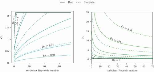
Figure 5 shows the model constants depending on the turbulent Reynolds number and the Damköhler number. The upper limit of the Damköhler number has virtually no effect on the model constants since they are always in the limit of the classical constant values in this range.

Figure 5. EDC Constants depending on $\mathrm{R}{\mathrm{e}}_{\mathrm{t}\mathrm{u}\mathrm{r}\mathrm{b}}$ and Damköhler number Da${ }_{\eta }$; Da${ }_{\eta }$ is ranging from 0.01 (lightest color) to 1 (darkest color) and plots are logarithmically spaced between

Numerical eigenvalue and eigenvector computation

For the chemical time scale definitions IETS and EVTS (see sections 3.8 and 3.9) the eigenvalues, and for EVTS also the eigenvectors, for a real nonsymmetric matrix have to be computed. The Jacobian matrix of the reaction system is in general neither sparse nor symmetric. The numerical calculation is usually done by first transforming the matrix into Hessenberg form and applying the eigenvalue search to this simplified matrix. The transformation can be conducted by a sequence of Householder transformations or by an elimination method analogous to Gaussian elimination with pivoting. Algorithmic details are presented in (Press et al. 2007; Wilkinson and Reinsch 1971). This algorithm needs approximately $5\left(N^3/3\right)$ operations (Press et al. 2007).

For the application in conjunction with the EDC, these operations need to be conducted at each time step and in each cell of the computational grid. This leads to long computational times which hinder practical applications of those eigenvalue based time scale formulations. Therefore, the IETS and EVTS will not be used in the flame simulations. Furthermore, the simple test cases showed that also simpler formulations approximate the analytically calculated chemical time scale well, section 4.1 and 4.2.

Numerical characterization of flame D

Sandia Flame D, a turbulent jet flame, is used to compare the time scales. Barlow and Frank (1998), Masri et al. (1996) provided detailed measurement data for this flame.

Although the modifications of the EDC, section 5.1, were suggested to improve the predictions for MILD combustion, they are also tested for the “classical” turbulent combustion regime to ensure their generality. As section 5.2 shows, for high turbulent Reynolds numbers and high Damköhler numbers the EDC model constants fall into the limit of the original EDC (Magnussen 2005).

The Flame was simulated in OpenFoam-6.x with an in-house code extension, based on the reactingFoam solver. The solver was modified to use the EDC-models from Parente and Bao. A wedge of the flame is simulated consisting of 5 170 cells. The $k-ϵ$ turbulence model (Jones and Launder 1972; Launder and Spalding 1974) was used with its original constants (Tannehill et al. 1984).

The suggested time scale formulations were tested with both, Parente’s and Bao’s EDC modification. The flame was simulated with the global Jones-Lindstedt mechanism (Jones and Lindstedt 1988) (see Table 1) and the detailed GRI-3.0 mechanism (Smith et al. 2018). This was done to study the effects of the difference in chemical time scale prediction on the flame simulation, because we saw already in the simplified test cases in section 4 that we get different results using a single-step and a comprehensive reaction mechanism.

Table 1. Methane combustion mechanism from Jones and Lindstedt (1988). Units in cm, s, cal and mol

reactions	A	$\beta$	$E_a$	reaction orders
CH4 + 0.5 O2 → CO + 2 H2	$7.820e13$	0	$30e3$	$[\mathrm{C}{\mathrm{H}}_4{]}^{0.5}[{\mathrm{O}}_2{]}^{1.25}$
CH4 + H2O → CO + 3 H2	$0.300e12$	0	$30e3$	$[\mathrm{C}{\mathrm{H}}_4][{\mathrm{H}}_2\mathrm{O}]$
H2 + 0.5 O2 ↔ H2O	$1.209e18$	−1	$40e3$	$[{\mathrm{H}}_2{]}^{0.25}[{\mathrm{O}}_2{]}^{1.5}$
CO + H2O ↔ CO2 + H2	$0.275e13$	0	$20e3$	$[\mathrm{C}\mathrm{O}][{\mathrm{H}}_2\mathrm{O}]$

Results using Jones-Lindstedt mechanism

The simulations using the time scale formulations IJTS, IRRTS and ETS failed to ignite the flame. The calculated characteristic chemical time scales were large and therefore, the Damköhler number was at the limit of Da = 0.01, which leads to low $C_{\gamma }$ and high $C_{\tau }$ values. This usually happens in MILD combustion and depicts a thickening of the flame front, (Parente et al. 2016), but is not known to occur in “classical” turbulent flames.

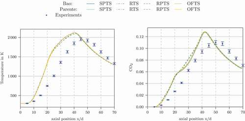
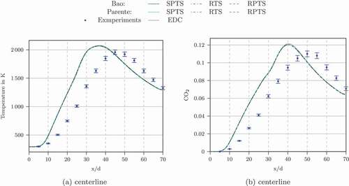
The simulations with the other time scale formulations (SPTS, RTS, RPTS and OFTS) gave results in line with the experimental data, see Figure 6. The results were also compared with the original EDC formulation. The original EDC results are not shown to avoid overlaps. They are very close to the modified ones.

Figure 6. Temperature and CO${ }_2$ concentration profiles at the centerline of Flame D calculated using the Jones-Lindstedt mechanism

Figure 7 shows the characteristic chemical time scales for the simulation domain. The profiles show a qualitative agreement of the different definitions. Only the RPTS method gives a time scale decrease in the flame zone. This is probably caused by a scarcity of product species/produced species in this region. The differences in the absolute values can be more clearly seen in Figure 8 and in the deviations of the Damköhler number.

Figure 7. Characteristic chemical time scale in Flame D calculated with different methods using the Jones-Lindstedt mechanism. Upper half: Bao’s formulation, lower half: Parente’s formulation

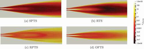
Figure 8. Profiles of the characteristic chemical time scale and the Damköhler number for Flame D simulated with the Jones-Lindstedt mechanism at different axial location

Figure 8 shows selected profiles of the characteristic chemical time scale and the Damköhler number. In some regions, especially outside the reaction zone, the Damköhler number is also at the lower limit with these time scale definitions. Low Damköhler values occur within the reaction zone for some time scale definitions. OFTS and RPTS even give Damköhler numbers below unity in this region. However, Figure 5 shows, that $C_{\tau }$ and $C_{\gamma }$ might reach their original values even with these low Damköhler numbers, when the turbulent Reynolds number is sufficiently large.

Results using GRI-3.0 mechanism

The OFTS, the IJTS, the IRRTS and ETS failed to ignite the flame also using the GRI-3.0 mechanism. Similar to the Jones and Lindstedt calculations (section 6.1) the Damköhler number was at its lower limit using those formulations.

Figure 9 shows the chemical time scales calculated with the methods SPTS, RTS and RPTS. The left half shows the simulation with Bao’s formulation and the right half with Parente’s.

Figure 9. Characteristic chemical time scale in Flame D calculated with different methods (SPTS, RTS, RPTS). Left: Bao’s formulation, Right: Parente’s formulation

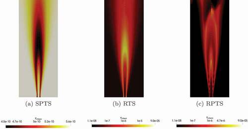
Figure 10. Profiles of the characteristic chemical time scale for Flame D simulated with GRI-3.0 at different radial and axial location(s). ${\tau }_{\mathrm{c}\mathrm{h}\mathrm{e}\mathrm{m}}$ calculated by the SPTS method is shown on the right axis in all the diagrams

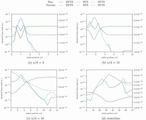
The SPTS method gives lower chemical time scales in the reaction zone, whereas the other two methods give higher chemical time scale values in the reaction zone. This might seem unreasonable, since the reactions proceed faster in the reaction zone and, therefore, ${\tau }_{\mathrm{c}\mathrm{h}\mathrm{e}\mathrm{m}}$ should be lower than in the area surrounding the flame. It can be argued, that the characteristic chemical time scale can not be estimated properly outside the reaction zone because the reaction rate is close to zero. Therefore, ${\tau }_{\mathrm{c}\mathrm{h}\mathrm{e}\mathrm{m}}$ takes default values in these regions, which do not correspond to the state of the chemical system. In the actual “flame region”, the SPTS method gives the lowest values inside the flame and higher values at the flame fronts, where oxidizer and methane mix. For the RTS method, ${\tau }_{\mathrm{c}\mathrm{h}\mathrm{e}\mathrm{m}}$ is slower at the flame front, while the RPTS method gives low values in this region. The trends of SPTS and RTS are similar in the flame and at the flame fronts.

Figure 10 and Figure 11 underline these observations for certain radial and axial profiles. It has to be noted, that the SPTS method gives time scale values orders of magnitudes lower than the RTS and RPTS method. Therefore, SPTS is shown on the right axis.

Figure 11. Temperature and CO${ }_2$ profiles at the centerline of Flame D calculated using GRI-3.0 mechanism

In general, the time scale definitions SPTS, RTS and RPTS run into the limits for the original EDC values $C_{\gamma }$ and $C_{\tau }$ with the complex reaction mechanism.

Comparison of the mechanisms

The difference between the formulation of Bao and Parente, section 5.1.1 and 5.1.2, are negligible compared to the differences induced by the different time scale formulations.

The IJTS, IRRTS and ETS methods modified the EDC constants in a way, that Flame D did not ignite in the simulation. The same holds true for the OFTS method in conjunction with the GRI-3.0 reaction mechanism. These time scale formulations should not be used in conjunction with the modified EDC, especially not for “classical” turbulent flames.

When comparing the definitions, which showed good results for Flame D, namely SPTS, RTS and RPTS, it has to be noted that they are strongly influenced by the reaction mechanism. Especially RTS and RPTS show different trends for the overall flame.

Numerical characterization of AJHC

To test the suggested EDC modifications for MILD conditions the Adelaide Jet in Hot Coflow (AJHC) Burner was chosen. It is a laboratory-scale burner, using methane and hydrogen. Dally, Karpetis, and Barlow (2002) published extensive measurement data of the flame, with different levels of oxygen in the coflow (3, 6 and 9%). The cases are named HM1, HM2 and HM3. For this study HM1 was simulated as a wedge with 19 500 cells using the $k$-$ϵ$ turbulence model with its original constants.

Compared to the Flame D simulations, a slightly different solver was used here to also account for differential diffusion effects. Christo and Dally (2005) showed that they play an essential role in MILD combustion simulations.

As for the classical combustion test case we employed two different reaction mechanisms, the Jones-Lindstedt mechanism (Jones and Lindstedt 1988) and the GRI-3.0 (Smith et al. 2018), as in section 6.1 and 6.2.

Results using Jones-Lindstedt mechanism

The Jones-Lindstedt mechanism (Table 1) was originally derived for methane oxidation, but it also incorporates hydrogen. It has already been used before for the simulation of hydrogen-methane flames, for example by Li et al. (2019).

The flame ignited only partially using the IRRTS formulation and extinction occurred, because the chemical time scales were large and lead to $\mathrm{D}\mathrm{a}=0.01$ in the entire domain. This seems too low, even for a MILD combustion flame.

Also, the results using ETS were not very satisfactory. The high values of the chemical time scales lead to extinction of the flame, despite initial ignition. Damköhler numbers ranged from $0.01$ to $1000$. Therefore, the failure of this method could not be clearly related to an incorrect prediction of the Damköhler number.

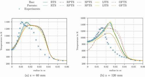
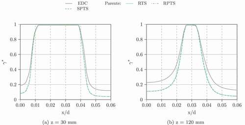
The temperature profiles using the other characteristic chemical time scale formulations in conjunction with Bao’s and Parente’s EDC modification are shown in Figure 12. They all show reasonable agreement for the profiles at the z = 4, 30 and 60 mm locations. For z = 120 mm we see differences between the formulations. Bao’s model in conjunction with IJTS underestimates the temperature. The flame in this simulation was not fully ignited. Using OFTS, the temperature peak was overestimated.

Figure 12. Radial temperature profiles at different locations for Adelaide Jet in Hot Coflow using the Jones-Lindstedt mechanism

Figure 14 shows the Damköhler number for the flame simulations. The method, which overpredict the temperature peak the most (OFTS), have lower Damköhler numbers, especially compared to SPTS and RTS definition. OFTS might overestimate the characteristic chemical time scale leading to Damköhler numbers being too low.

The differences between the temperatures (Figure 12) are related to the chemical time scale definitions primarily and not to the EDC formulation (Bao vs. Parente). Only the IJTS method gives significantly different results for the two EDC constant formulations. Figure 13 reveals that those differences in temperature and other major scalars are caused by differences in ${\gamma }^{\ast }$ and ${\tau }^{\ast }$. The different ${\gamma }^{\ast }$ and ${\tau }^{\ast }$ originate from the variable EDC constants $C_{\tau }$ and $C_{\gamma }$ (Equation (26)(26) ${\gamma }_L=C_{\gamma }{\left(\frac{ϵ\nu }{k^2}\right)}^{1/4}={\left({\gamma }^{\ast }\right)}^{\left(1/3\right)}$(26) and Equation (27)(27) ${\dot{m}}^{\ast }=\frac{1}{C_{\tau }}{\left(\frac{ϵ}{\nu }\right)}^{1/2}=\frac{1}{{\tau }^{\ast }}$(27) ). The variation in those constants arises from the different chemical time scale approximations .

Figure 13. Radial profile for ${\gamma }^{\ast }$ and ${\tau }^{\ast }$ s at z = 120 mm for Adelaide Jet in Hot Coflow using the Jones-Lindstedt mechanism

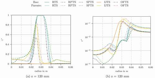
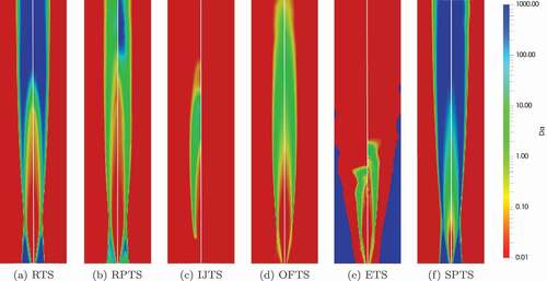
Figure 14. Damköhler numbers for the AJHC simulation domain (r = 0–127 mm, z = 0–1 m) using the Jones-Lindstedt mechanism; left: Parente’s formulations, right = Bao’s formulation

Results using GRI-3.0 mechanism

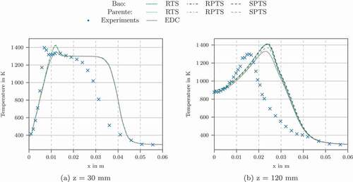
Similarly to the simulation of Flame D using GRI-3.0 mechanism, only the RTS, RPTS and SPTS formulations show good results. The OFTS, IJTS, and IRRTS methods run into the limit of $\mathrm{D}\mathrm{a}=0.01$ which lead to a failed ignition of the flame. Figure 15 shows the time scale methods which gave accurate results. For comparison, also the results using the original EDC model are shown. The modified models predict the temperature better for the profile at z = 120 mm (Figure 15b) but for the profile at z = 60 mm (Figure 15a) and z = 30 mm the modified models are superior.

Figure 15. Radial temperature profiles at different locations for Adelaide Jet in Hot Coflow using GRI-3.0 mechanism

Figure 16 shows selected chemical time scale profiles and the Damköhler number on the computational domain. The Damköhler number obtained with the SPTS method is not shown, since $\mathrm{D}\mathrm{a}=1000$ in the whole domain. This seems unreasonable for a MILD combustion flame and suggests that the SPTS method underestimates the characteristic chemical time scale in combination with the GRI-3.0 mechanism.

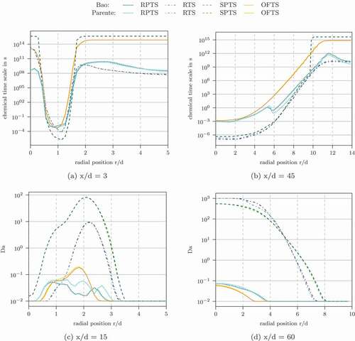
Figure 16. Chemical time scale profiles for AJHC using GRI-3.0 ((a) and (b) – SPTS on the right axis) and the Damköhler number ((c) and (d)) (left: Parente’s formulation, right plane: Bao’s formulation)

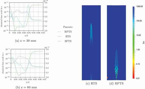
The characteristic chemical time scale profiles for z = 30 mm and z = 60 mm in Figure 16a and 16b (only the results with Parente’s formulation are shown, since the results between the formulations do not differ significantly) show that SPTS gives values, which are orders of magnitudes lower than the others. This leads to the high Damköhler numbers. The other methods (RTS and RPTS) estimate lower characteristic chemical time scales and lead to Damköhler numbers, which seem high for a MILD combustion flame.

The differences between the original EDC formulation and the modified constants (Figure 15) is related to a difference in${\gamma }^{\ast }$. The fine structure residence time values ${\tau }^{\ast }$ are nearly equivalent for all the cases. Figure 17 shows the differences in ${\gamma }^{\ast }$ for selected profiles. (Only the results from Parente are depicted here, because Bao’s formulation shows very similar results for ${\gamma }^{\ast }$.) The modified constants yield different results compared to the original EDC which agrees well with the differences seen in the temperature profiles (Figure 15).

Figure 17. Radial profiles of ${\gamma }^{\ast }$ at different locations for Adelaide Jet in Hot Coflow using GRI-3.0 mechanism

Comparison of the mechanisms

Figure 18 compares the characteristic chemical time scales calculated with the Jones-Lindstedt and GRI-3.0 mechanism. For the definitions shown, the characteristic chemical time scales in conjunction with GRI-3.0 are orders of magnitudes lower than with the Jones-Lindstedt mechanism.

Figure 18. Comparison of chemical time scale profiles using Jones-Lindstedt and GRI-3.0 mechanism, In (c) the results from GRI-3.0 are shown on the right axis

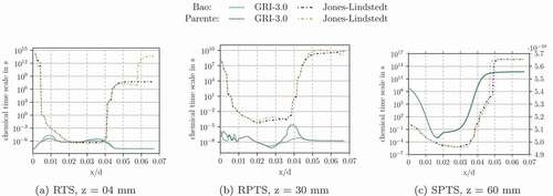
If we consider the chemical time scale as a value to characterize a flame, this depicts a problem with the available time scale approximations: They are highly dependent on the reaction mechanism. These variations could be eliminated by always using global mechanisms to approximate the characteristic chemical time scale.

Conclusion

We presented various numerically efficient characteristic chemical time scale definitions – ranging from simple analytical expressions to complex eigenvalue based formulations. They were compared for a simple test case, where also an analytical eigenvalue can be computed. For this case, they all predict the trend of the time scales reasonably well. We see that, there are two groups, incorporating two different trends, though. One group, with the eigenvalue based methods approximate the analytic solution better.

Using a more complex reaction mechanism, the time scale predictions vary by several orders of magnitude and give different trends for the test case. Due to the lack of an analytical solution, the values can not be verified. Based on the simple test case, a good choice for the time scale approximation are the eigenvalue based definitions, for example EVTS, if fast computation of the time scale is not essential.

For CFD applications, such as the EDC model variations, the characteristic chemical time scale needs to be computed in every cell at every time step. In this case, eigenvalue based methods are not viable at the moment due to the numerical effort. Therefore, only the simpler formulations, without the need to compute eigenvalues, were tested for the flame simulations with the modified EDC.

The RTS, RPTS and SPTS seem to provide a suitable characteristic chemical time scale definition for combustion simulations. These formulations gave reasonable predictions for all test cases. Nevertheless, differences were observed and a great influence of the mechanism complexity on the chemical time scale was shown. This also leads to varying EDC model constants and consequently, differing simulation results.

Therefore, we suggest to use a simple, preferably one-step reaction mechanism, for the chemical time scale calculation, while using a complex chemical mechanism for the simulation. This enables comparable and consistent results, even when using chemical mechanisms with different levels of complexity. A detailed mechanism can be used to calculate temperatures and species concentrations, and a one step mechanism should be used to approximate the chemical time scale.

Parente et al. (2011) also used a single-step reaction mechanism for the determination of the chemical time scale and more complex ones for the calculation of the combustion progress. Computational time was their reason for the global mechanism and no results using complex mechanisms were presented.

Within the tested time scale methods, the RTS, and SPTS gave the best results. The RPTS could also be a good choice, but shows some deficiencies since its formulation is only based on product species. Therefore, we recommend to use the RTS or SPTS formulation based on a single-step reaction mechanism for the modified EDC.

Disclosure statement

The authors declare no conflict of interest.

Additional information

Funding

The authors gratefully acknowledge the funding support of K1-MET GmbH, metallurgical competence center. The research program of the competence center K1-MET is supported by COMET (Competence Center for Excellent Technologies), the Austrian program for competence centers. COMET is funded by the Federal Ministry for Transport, Innovation and Technology, the Federal Ministry for Digital and Economic Affairs, the province of Upper Austria, Tyrol, and Styria. Apart from funding, the project activities are financed by the industrial partners Primetals Technologies Austria, voestalpine Stahl and voestalpine Stahl Donawitz;Österreichische Forschungsförderungsgesellschaft [869295].The authors acknowledge the TU Wien University Library for financial support through its Open Access Funding Program.

References

- Ansys-Inc. n.d. Ansys fluent theory guide release 17.0. Canonsburg, PA, USA: Ansys Inc.
- Bao, H. (2017). Development and validation of a new Eddy Dissipation Concept (EDC) model for MILD combustion, Master’s thesis, Delft University of Technology.
- Barlow, R. S., and J. H. Frank. 1998. Effects of turbulence on species mass fractions in methane/air jet flames. Twenty-Seventh Symp. (Int.l) Combust. 27:1087–95.
- Bösenhofer, M., E.-M. Wartha, C. Jordan, and M. Harasek. 2018. The eddy dissipation concept-analysis of different fine structure treatments for classical combustion. Energies 11:7.
- Caudal, J., B. Fiorina, M. Massot, B. Labégorre, N. Darabiha, and O. Gicquel. 2013. Characteristic chemical time scales identification in reactive flows. Proc. Combust. Inst. 34 (1):1357–64.
- Cavaliere, A., and M. de Joannon. 2004. MILD combustion. Progr. Energy Combust. Sci. 30 (4):329–66.
- Christo, F. C., and B. B. Dally. 2005. Modeling turbulent reacting jets issuing into a hot and diluted coflow. Combust. Flame 142 (1–2):117–29.
- Dally, B., A. Karpetis, and R. Barlow. 2002. Structure of turbulent non-premixed jet flames in a diluted hot coflow. Proc. Combust. Inst. 29 (1):1147–54.
- De, A., E. Oldenhof, P. Sathiah, and D. Roekaerts. 2011. Numerical simulation of Delft- Jet-in-Hot-Coflow (DJHC) flames using the eddy dissipation concept model for turbulence- chemistry interaction. Flow Turbul. Combust. 87,4:537–67.
- Ertesvåg, I. S. 2019. Analysis of some recently proposed modifications to the Eddy Dissipation Concept (EDC) analysis of some recently proposed modifications to the Eddy Dissipation Concept (EDC). Combust. Sci. Technol. 1–29.
- Ertesvåg, I. S., and B. F. Magnussen. 1999. The eddy dissipation turbulence energy cascade model. Combust. Sci. Technol. 159 (1):213–35.
- Evans, M. J., P. R. Medwell, and Z. F. Tian. 2015. Modeling lifted jet flames in a heated coflow using an optimized Eddy Dissipation Concept model. Combust. Sci. Technol. 187 (7):1093–109.
- Evans, M. J., C. Petre, P. R. Medwell, and A. Parente. 2019. Generalisation of the eddy- dissipation concept for jet flames with low turbulence and low Damköhler number. Proc. Combust. Inst. 37:4497–505.
- Farokhi, M., and M. Birouk. 2016. Application of eddy dissipation concept for modelling biomass combustion, part 2: Gas-phase combustion modeling of a small-scale fixed bed furnace. Energy Fuels 30 (12):10800–08.
- Gerschgorin, S. 1931. Über die Abgrenzung der Eigenwerte einer Matrix. Bulletin de l’Académie des Science de l’URSS. Classe des science mathématiques et na 6:749–54.
- Gilbert, R. G., K. Luther, and J. Troe. 1983. Theory of thermal unimolecular reactions in the fall-off range. ii. weak collision rate constants. Berichte der Bunsengesellschaft fr physikalische Chemie 87 (2):169–77.
- Glassmaker, N. J. 1999. Intrinsic low-dimensional manifold method for rational simplification of chemical kinetics.
- Golovitchev, V. I., and J. Chomiak (2001). Numerical modeling of high temperature air ”flameless” combustion, The 4th International Symposium on High Temperature Air Combustion and Gasification, Rome, Italy.
- Golovitchev, V. I., and N. Nordin. 2001. Detailed chemistry spray combustion model for the KIVA code by. Int. Multidimension. Engine Model. User’s Group Meeting SAE Congr.
- Goodwin, D. G., H. K. Moffat, and R. L. Speth (2017). Cantera: An object-oriented software toolkit for chemical kinetics, thermodynamics, and transport processes, http://www.cantera.org.Version 2.3.0.
- Gran, I. R., and B. F. Magnussen. 1996. A numerical study of a bluff-body stabilized diffusion flame. Part 2. influence of combustion modeling and finite-rate chemistry. Combust. Sci. Technol. 119 (1–6):191–217.
- Isaac, B. J. (2014). Principal component analysis-based combustion models, PhD thesis, The University of Utah. http://content.lib.utah.edu/cdm/singleitem/collection/etd3/id/2932/rec/1962
- Isaac, B. J., A. Parente, C. Galletti, J. N. Thornock, P. J. Smith, and L. Tognotti. 2013. A novel methodology for chemical time scale evaluation with detailed chemical reaction kinetics. Energy Fuels 27 (4):2255–65.
- Jones, W., and R. Lindstedt. 1988. Global reaction schemes for hydrocarbon combustion. Combust. Flame 78:233–49.
- Jones, W. P., and B. E. Launder. 1972. The prediction of laminarization with a two-equation model of turbulence. Int. J. Heat Mass Transfer 15:301–14.
- Lam, S. H., and D. A. Goussis. 1991. Conventional asymptotics and computational singular perturbation for simplified kinetics modelling. In Reduced kinetic mechanisms and asymptotic approximations for methane-air flames, chapter 10. Berlin, Heidelberg: Springer Verlag.
- Launder, B. E., and D. B. Spalding. 1974. The numerical computation of turbulent flows. Comput. Methods Appl. Mech. Eng. 3:269–89.
- Lewandowski, M. T., I. S. Ertesvåg, and J. Pozorski (2017). Influence of the reactivity of the fine structures in modelling of the jet-in-hot-coflow flames with the eddy dissipation concept, 8th European Combustion Meeting, Dubrovnik, Croatia.
- Li, Z., A. Cuoci, and A. Parente. 2019. Large eddy simulation of MILD combustion using finite rate chemistry: Effect of combustion sub-grid closure. Proc. Combust. Inst. 37:4519–29.
- Li, Z., A. Cuoci, A. Sadiki, and A. Parente. 2017. Comprehensive numerical study of the adelaide jet in hot-coflow burner by means of RANS and detailed chemistry. Energy 139:555–70.
- Li, Z., M. Ferrarotti, A. Cuoci, and A. Parente. 2018. Finite-rate chemistry modelling of non-conventional combustion regimes using a partially-stirred reactor closure: Combustion model formulation and implementation details. Appl. Energy 225:637–55.
- Lindemann, F. A., S. Arrhenius, I. Langmuir, N. R. Dhar, J. Perrin, and L. W. C. McC. 1922. Discussion on the radiation theory of chemical action. Trans. Faraday Soc. 17:598–606.
- Løvås, T., F. Mauss, C. Hasse, and N. Peters. 2002. Development of adaptive kinetics for application in combustion systems. Proc. Combust. Inst. 29:1403–10.
- Magnussen, B. F. (1981). On the structure of turbulence and a generalized eddy dissipation concept for chemical reaction in turbulent flow, 19th Aerospace Sciences Meeting, St. Louis, MO, USA.
- Magnussen, B. F. (2005). The eddy dissipation concept—A bridge between science and technology, ECCOMAS Thematic Conference on Computational Combustion, Lisbon, Portugal.
- Masri, A. R., R. W. Dibble, and R. S. Barlow. 1996. The structure of turbulent nonpremixed flames revealed by Raman-Rayleigh-LIF measurements. Progr. Energy Combust. Sci. 22:307–62.
- Nagy, T., and T. Turànyi. 2009. Relaxation of concentration perturbation in chemical kinetic systems. React. Kinet. Catal. Lett. 96 (2):269–78.
- Parente, A., M. R. Malik, F. Contino, A. Cuoci, and B. B. Dally. 2016. Extension of the eddy dissipation concept for turbulence/chemistry interactions to MILD combustion. Fuel 163:98–111.
- Parente, A., J. C. Sutherland, B. B. Dally, L. Tognotti, and P. J. Smith. 2011. Investigation of the MILD combustion regime via principal component analysis. Proc. Combust. Inst. 33 (2):3333–41.
- Press, W. H., S. A. Teukolsky, W. T. Vetterling, and B. P. Flannery. 2007. Numerical recipes - the art of scientific computing. Cambridge: Cambridge University Press.
- Prüfert, U., F. Hunger, and C. Hasse. 2014. The analysis of chemical time scales in a partial oxidation flame. Combust. Flame 161 (2):416–26.
- Rehm, M., P. Seifert, and B. Meyer. 2009. Theoretical and numerical investigation on the EDC-model for turbulence–chemistry interaction at gasification conditions. Comput. Chem. Eng. 33 (2):402–07.
- Ren, Z., and G. M. Goldin. 2011. An efficient time scale model with tabulation of chemical equilibrium. Combust. Flame 158 (10):1977–79.
- Smith, G. P., D. M. Golden, M. Frenklach, N. W. Moriarty, B. Eiteneer, M. Goldenberg, C. T. Bowman, R. K. Hanson, S. Song, W. C. Gardiner Jr., et al. (2018). GRI-Mech 3.0.
- Stewart, P., C. Larson, and D. Golden. 1989. Pressure and temperature dependence of reactions proceeding via a bound complex. 2. application to 2ch3 c2h5 + h. Combust. Flame 75 (1):25–31.
- Tannehill, J. C., D. A. Anderson, and R. H. Pletcher. 1984. Computational fluid mechanics and heat transfer. Second. Boca Raton: CRC Press.
- Tomlin, A. S., L. Whitehouse, and M. J. Pilling. 2002. Low-dimensional manifolds in tropospheric chemical systems. Faraday Discuss. 120:125–46.
- Troe, J. 1983. Theory of thermal unimolecular reactions in the fall-off range. i. strong collision rate constants. Berichte der Bunsengesellschaft fr physikalische Chemie 87 (2):161–69.
- Tsang, W., and J. T. Herron. 1991. Chemical kinetic data base for propellant combustion i. reactions involving no, no2, hno, hno2, hcn and n2o. J. Phys. Chem. Ref. Data 20 (4):609–63.
- Weller, H., G. Tabor, H. Jasak, and C. Fureby. 1998. A tensorial approach to computational continuum mechanics using object-oriented techniques. Comput. Phys. 12:6.
- Westbrook, C. K., and F. L. Dryer. 1981. Simplified reaction mechanisms for the oxidation of hydrocarbon fuels in flames. Combust. Sci. Technol. 27 (1–2):31–43.
- Wilkinson, J., and C. Reinsch. 1971. Handbook for automatic computation, vol. II, linear algebra. Springer-Verlag Berlin Heidelberg, New York.