A Skeletal Mechanism for MILD Combustion of n-Heptane/Air Mixtures

ABSTRACT

Moderate, intense or low-oxygen dilution (MILD) Combustion has many attributes such as low emissions, noiseless combustion with high thermal efficiency which are attractive for greener combustion systems. Past studies investigated flow and chemical kinetics effects in establishing this combustion mode for methane-air mixtures. Many of the practical fuels are large hydrocarbons and hence this study aims to develop a skeletal mechanism suitable for turbulent MILD combustion simulations of n-heptane/air. Computer Assisted Reduction Mechanism approach is employed to develop a mechanism involving 36 species and 205 reactions, which is validated for wide range of conditions using measurements or results obtained from a comprehensive mechanism. This mechanism is found to be excellent for predicting both ignition delay times and flame speeds for MILD conditions. The OH* and CH* obtained using quasi-steady state assumptions agree well with those obtained using the comprehensive mechanism with these chemiluminescent species. The performance of the skeletal mechanism for turbulent MILD combustion simulation is tested using Unsteady Reynolds Averaged Navier-Stokes (URANS) simulations with a finite-rate chemistry model. The computed statistics of temperature and $\mathrm{O}\mathrm{H}$ number density agree quite well with measurements for highly diluted combustion cases.

KEYWORDS:

• n-heptane
• combustion kinetics
• skeletal mechanism
• computer assisted reduction mechanism (CARM)
• MILD combustion
• finite rate chemistry model

Introduction

Moderate, intense or low-oxygen dilution (MILD) combustion features low emissions, high efficiency, uniform thermal field, almost quiet and stable combustion with high fuel flexibility (Cavaliere and de Joannon 2004; Katsuki and Hasegawa 1998; Wünning and Wünning 1997). These are attractive for environmentally friendly combustion systems and hence MILD combustion research is attracting increased interest (Arghode, Gupta, Bryden 2012; de Joannon, Sorrentino, Cavaliere 2012; Khalil and Gupta 2017; Perpignan, Rao, Roekaerts 2018; Weber, Gupta, Mochida 2020). This combustion is also known as Colorless Distributed Combustion (CDC) and so, ascertaining its presence requires some visual imaging either a photograph or chemiluminescent imaging of the combustion zone in addition to other measurements (Arghode and Gupta 2010). One cannot use only combustor exit temperature and emission measurements to claim presence of MILD combustion. This is because combustor aerodynamics (Arghode and Gupta 2010; Arghode, Gupta, Bryden 2012; Khalil and Gupta 2014, 2017), local thermochemical conditions (Arghode, Gupta, Bryden 2012; Karyeyen, Feser, Gupta 2019) and operating pressure (Khalil and Gupta 2015; Ye et al. 2015) were shown to strongly affect conditions conducive for CDC. The combustion was observed to depart from MILD regime when the fuel and air were injected separately as in non-premixed mode (Khalil and Gupta 2015) or fuel is changed at elevated pressures (Ye et al. 2015). This is because of inadequate mixing of fuel and air with hot diluents or a change in the chemical time scale due to the fuel change. Typically, MILD regime is achieved using high speed jets to create strong recirculating flows enhancing fuel/air mixing with hot burnt gases. These gases act as diluents to achieve homogeneous combustion resulting in uniform temperature field with substantially low levels of CO, soot and thermal $\mathrm{N}{\mathrm{O}}_x$ production (Cavaliere and de Joannon 2004; Katsuki and Hasegawa 1998; Wünning and Wünning 1997).

Fuel–air mixture temperature, $T_r$, is larger than the ignition temperature, $T_{\mathrm{i}\mathrm{g}\mathrm{n}}$, and the overall temperature rise across reaction zone $\mathrm{\Delta }T$ is smaller than $T_{\mathrm{i}\mathrm{g}\mathrm{n}}$ in MILD combustion (Cavaliere and de Joannon 2004). Typically, $T_r$ is above 1100 K and this combustion is different from HiTAC, High Temperature Air Combustion, which has $\mathrm{\Delta }T>T_{\mathrm{i}\mathrm{g}\mathrm{n}}$ (Weber, Gupta, Mochida 2020). The application of CDC technology is demonstrated for practical systems such as furnace (Galletti, Parente, Tognotti 2007; Parente, Galletti, Tognotti 2008), gas turbine (Kruse et al. 2015; Perpignan, Rao, Roekaerts 2018) and hybrid solar thermal system (Chinnici et al. 2017). The salient characteristics of this combustion were investigated using different laboratory-scale burners such as Jet in Hot Coflow (JHC) burners of Dally, Karpetis, and Barlow (2002) and De et al. (2011), reverse-flow adiabatic arrangement of Graça et al. (2013) and Ye et al. (2015), cylindrical non-adiabtic combustor used by Veríssimo, Rocha, and Costa (2011) and a cyclonic burner of Sorrentino et al. (2016, 2019). These studies considered atmospheric pressure and simple gaseous fuels like methane, hydrogen, ethylene, propane and ammonia, showing some common characteristics such as broadened heat releasing regions, weakened correlation between maximum reaction rate locations and stoichiometric mixture fraction as well as the disappearance of pyrolysis region (de Joannon et al. 2009; de Joannon, Sorrentino, Cavaliere 2012).

Despite the high fuel flexibility of CDC noted by Khalil and Gupta (2017), Karyeyen, Feser, and Gupta (2019) and, Medwell and Dally (2012), few studies observed that CDC of complex fuels, such as oxygenated fuels and long-chain alkanes, led to distinct features like increased pollutants emission and appearance of visible flames. Also, higher dilution level was required to achieve CDC for these complex fuels compared to those for simple fuels (Li et al. 2021a; Reddy et al. 2014; Saha et al. 2014; Weber, Smart, Vd Kamp 2005; Ye et al. 2015).

CDC occurs only under appropriate thermochemical condition even for methane as noted by Arghode, Gupta, and Bryden (2012), Khalil and Gupta (2017), and Karyeyen, Feser, and Gupta (2019). Hence, fuel chemistry plays a vital role in the inception of sustained CDC as demonstrated in direct numerical simulation (DNS) of Doan and Swaminathan 2019a;Doan and Swaminathan 2019b) and thus the use of one-step reaction with high activation energy commonly employed for combustion analyses is insufficient to investigate CDC. Both comprehensive and skeletal mechanisms for simple hydrocarbon like $\mathrm{C}{\mathrm{H}}_4$ were developed and tested in past studies. However, there aren’t skeletal mechanisms suitable for numerical studies of turbulent CDC of large hydrocarbons such as $n$-heptane.

Mehl et al. (2011) developed a comprehensive mechanism involving 654 species and 2827 reactions for 3 to 50 atm and $650\le T_r\le 1200K$, which are relevant for IC engines and showed a good agreement between computed and measured ignition delay times. Zhang et al. (2016) used the sub $n$-heptane mechanism of Mehl et al. (2011) along with C0-C4 sub-mechanism of Zhou et al. (2016) and Li et al. (2017a) to develop a comprehensive mechanism with 1268 species and 5336 reactions to predict not only the ignition delay times but also the laminar flame speeds and species concentrations over a wide range of conditions, 1 to 55 atm and $500\le T_r\le 1412$ K, for $n$-heptane oxidation. Comprehensive mechanisms involving several hundreds of species and many thousands of reactions were also developed and tested in past studies for $n$-heptane/air combustion, for example see the studies of Pelucchi et al. (2014) and Seidel et al. (2015).

These comprehensive mechanisms are required for capturing salient characteristics such as the negative temperature coefficient (NTC) behavior and chemical species responsible for it. Such investigations are possible only for laminar conditions and using these mechanisms for turbulent combustion simulations is impractical. This is specifically so for three-dimensional DNS and Large Eddy Simulation (LES) and thus a skeletal mechanism is typically used as in the past studies of Minamoto et al. (2014), Doan and Swaminathan (2019a), Li, Cuoci, and Parente (2019), Li et al. (2021b), and Bhaya, De, and Yadav (2014) for CH₄–air MILD combustion. Several skeletal mechanisms involving 70 to 100 species are available for liquid hydrocarbons (Liu et al. 2012; Lu and Law 2008; Ra and Reitz 2008; Wang, Yao, Reitz 2013; Yoo et al. 2011; Zhen, Wang, Liu 2016), which are targeted toward primary reference fuels (PRFs) with iso-octane and $n$-heptane mixtures (Liu et al. 2012; Ra and Reitz 2008; Wang, Yao, Reitz 2013; Zhen, Wang, Liu 2016). Hence, these mechanisms are unsuitable for DNS and LES of turbulent CDC of $n$-heptane. Past experiences with DNS of CH₄-air MILD combustion by Minamoto et al. (2014) and Doan and Swaminathan (2019a) suggest that a mechanism with about 40 species would be a good compromise between the computational cost and chemical detail. However, the abilities of such a mechanism to capture the chemical complexities of $n$-heptane/air MILD combustion is yet to be investigated. Furthermore, past DNS studies demonstrated that both autoignition and flame propagation are present in MILD combustion as its distinctive feature Doan and Swaminathan 2019a, Doan and Swaminathan 2019b; Minamoto et al. 2014; Minamoto and Swaminathan 2014). Hence, a skeletal mechanism for CDC should be able to capture the variations of both ignition delay time, $\tau$, and flame speed, $S_L$, with $T_r$, pressure, equivalence ratio and dilution.

It is common to consider either $\tau$ or $S_L$ for developing a skeletal mechanism depending on its intended use. Two mechanisms involving 41 species were developed for IC engine conditions (Liu et al. 2012; Ra and Reitz 2008) and they have not been tested for conditions relevant for MILD regime. Hence, the objectives of this study are to

1. Test the suitability of the 41-species mechanisms of Ra and Reitz (2008) and Liu et al. (2012) for MILD regime and develop, if required, a suitable skeletal mechanism for MILD combustion of $n$-heptane/air mixtures using CARM (Computer Assisted Reduction Mechanism) methodology (Chen 1988, 2001; Tham, Bisetti, Chen 2008; Chen and Tham 2008; Chen et al. 2017b; Chen and Chen 2018);

2. Validate the new skeletal mechanism using experimental data, if it is available, or results of a comprehensive mechanism; and

3. Evaluate the suitability of the new skeletal mechanism for turbulent MILD combustion simulations using finite rate chemistry models and experimental results for pre-vaporized $n$-heptane/air MILD combustion.

It is worth noting that the two requirements, $T_r>T_{\mathrm{i}\mathrm{g}\mathrm{n}}$ and $\mathrm{\Delta }T<T_{\mathrm{i}\mathrm{g}\mathrm{n}}$ for MILD combustion cannot be met over temperature range exhibiting low-temperature ignition for large hydrocarbons such as $n$-heptane. The low-temperature ignition, commonly known as NTC (negative temperature coefficient), regime predominantly involves breakdown of large fuel molecule into smaller ones. This process continues to high-temperature ignition/combustion where the complete oxidations of carbon and hydrogen to CO₂ and H₂O occur.

This paper is organized as follows. CARM methodology is described briefly in Section 2 along with the new skeletal mechanism for $n$-heptane/air mixtures. This mechanism is developed carefully for a wide range of conditions, specifically the dilution level, relevant for MILD regimes. The validation of this mechanism for $\tau$ and $S_L$ are presented in Sections 3.1 and 3.2 respectively. The chemiluminescent species such as $\mathrm{O}{\mathrm{H}}^{\ast }$ and $\mathrm{C}{\mathrm{H}}^{\ast }$ obtained using quasi-steady state assumptions (QSSA) along with the new skeletal mechanism are presented and compared to the results from the comprehensive mechanism in Section 3.3. The results of turbulent MILD combustion simulations involving the new skeletal mechanism are described in Section 3.4 and the conclusions of this study are summarized in the final section.

Brief description of CARM methodology

The Computer Assisted Reduction Mechanism (CARM) (Chen 1988, 2001; Tham, Bisetti, Chen 2008; Chen and Tham 2008; Chen et al. 2017b; Chen and Chen 2018) approach automates the process of mechanism reduction using methodologies such as Directed Relation Graph with Error Propagation (DRGEP) (Niemeyer and Sung 2011; Pepiot-Desjardins and Pitsch 2008), Targeted Search Algorithm (TSA) (Tham, Bisetti, Chen 2008) and QSSA (Chen 1988; Chen and Tham 2008).

Starting from the high-temperature part of the comprehensive mechanism of Zhang et al. (2016) with 252 species and 1931 reaction, DRGEP method is used as first reduction step with target species of fuel, major products and $\mathrm{H}$, allowing a cutoff threshold value of 0.01. The target set consists of 336 autoignition conditions with pressures at 1 and 10 atm, equivalence ratios of 0.7, 1.0, and 1.3, 28 values of $T_r$ ranging from 550 to 1450 K, and two dilution levels of 0% and 40%.

A starting skeletal mechanism with high accuracy for flame speeds is generated and this is used subsequently to determine $S_L$ variations for MILD conditions. To get this starting mechanism, a set of species important for $S_L$ predictions is identified using typical sensitivity analysis for $S_L$ with respect to species as suggested by Chen and Chen (2018). For this sensitivity analysis, the thermo-chemical and thermo-physical conditions of reactant mixture are kept in the ranges noted above which are of interest for MILD combustion applications. Next, the trial-and-error brute force method TSA of Tham, Bisetti, and Chen (2008) is applied on the starting skeletal mechanism for further reduction. Species with relative error larger than $10\mathrm{\%}$ in autoignition delay will be kept or otherwise removed. The species set required for flame speed is kept when using TSA. Finally, a skeletal mechanism with 36 species and 205 steps is obtained¹ and the various steps described above for this mechanism reduction is depicted using a flow chart shown in Figure 1

Figure 1. Flow chart for mechanism reduction.

Also, possible violations of collision limits for bi-molecular reactions are calculated following Chen, Wang, and Wang (2017a) and using the kinetic preprocessor of OpenSMOKE++ (Cuoci et al. 2015) and it is found that only one reaction, backward step of $2C2H4\iff C2H5+C2H3$, exceeds the collision limit by about 85% for only $T=300$ K. The QSSA is used to obtain a set of 31 intermediate species, such as OH*, CH*, C, and C2H, etc., in the post-processing step using a computer routine generated by CARM.

The conditions for validation are chosen carefully to cover ranges relevant for potential MILD combustion applications: the reactant mixture equivalence ratio, $\varphi$, ranges from 0.7 to 1.6 with pressure varying from 1 to 10 atm and dilution level, $\alpha$, from 0 to $50\mathrm{\%}$ in steps of $10\mathrm{\%}$ for both $\tau$ and $S_L$ calculations. The dilution level is defined as the ratio of $\left(\mathrm{C}{\mathrm{O}}_2+{\mathrm{H}}_2\mathrm{O}\right)$ mass in the reactant mixture to total mass of the mixture which is the sum of diluents, fuel, and air masses in the reactant mixture. For $S_L$ calculations, the mixture temperature is varied from 298 to $930\mathrm{K}$. The mixture temperature for $\tau$ calculations vary in the range of $950\le T_r\le 1450\mathrm{K}$, excluding NTC region. Indeed, high molecular weight hydrocarbons such as $n$-heptane can have low $T_{\mathrm{i}\mathrm{g}\mathrm{n}}$, about 500 K, giving low/intermediate temperature ignition which is also known as low-temperature combustion (LTC) (Ju 2021). It is well understood from past studies that LTC is likely to continue to high temperatures to complete the oxidation of carbon and hydrogen to their final products. The overall temperature rise, after the high-temperature oxidation, would be many hundreds of Kelvin which would violate the requirement for MILD combustion, ie., $\mathrm{\Delta }T<T_{\mathrm{i}\mathrm{g}\mathrm{n}}$. As noted earlier, this temperature raise is not for the entire combustor but it is across the local reaction zones. It may be possible to select experimental conditions with sufficiently large dilution through exhaust recirculation and short combustor residence time so that the average temperature raise across the entire combustor is lower than $T_{\mathrm{i}\mathrm{g}\mathrm{n}}$ with low NO $x$ emission at the combustor exit. This may be insufficient to say that the turbulent combustion is in MILD/CDC regime or not, without detailed temperature measurements or an appropriate imaging across the combustion zone. Nevertheless, the low temperature ignition is important for HiTAC conditions which is not the focus here.

Results and discussion

The performances of the 36-species skeletal mechanism, presented in the previous section, is tested and described below for its ability to capture both $\tau$ and $S_L$ for a range of thermo-chemical and thermo-physical conditions of interest for CDC. Also, the variations of chemiluminescent species such as $\mathrm{O}{\mathrm{H}}^{\ast }$ and $\mathrm{C}{\mathrm{H}}^{\ast }$ obtained using the $n$-heptane comprehensive mechanism of Zhang et al. (2016) with $\mathrm{O}{\mathrm{H}}^{\ast }$ and $\mathrm{C}{\mathrm{H}}^{\ast }$ reactions from Kathrotia et al. (2012) are compared to those obtained from QSSA involving chemical species in the 36-species skeletal mechanism. This comparative analysis is performed for MILD combustion conditions. The use of this skeletal mechanism for turbulent MILD combustion simulations is also tested and discussed in this section.

Validation for ignition delay times

A constant volume adiabatic reactor model in the Cantera package (Goodwin, Moffat, Speth 2017) is used to compute $\tau$, which are obtained as the time corresponding to the maximum $\mathrm{d}{\mathrm{Y}}_{\mathrm{O}\mathrm{H}}/dt$. The ignition delay times based on $\mathrm{d}{\mathrm{Y}}_{\mathrm{C}{\mathrm{H}}^{\ast }}/dt$ were also tested and compared with those obtained using $\mathrm{d}{\mathrm{Y}}_{\mathrm{O}\mathrm{H}}/dt$, and no large discrepancy was observed. Since CH* is unavailable as a species in the skeletal mechanisms, OH is used to calculate $\tau$ for all the cases discussed here. The results obtained using the comprehensive high-temperature kinetics described by Zhang et al. (2016) and experimental data from Ciezki and Adomeit (1993), Gauthier, Davidson, and Hanson (2004), Shen et al. (2009), and Campbell et al. (2015) are used to verify and validate the 36-species skeletal mechanism for its ability to predict $\tau$. Some of these experimental data were also used by Ra and Reitz (2008) and Liu et al. (2012) to check their 41-species skeletal mechanisms.

Figure 2 shows $\tau$ plotted as a function of $1000/T_r$ and the temperature range excludes NTC region. These results are shown for undiluted $n$-heptane/air mixtures. Values of $\tau$ obtained using the 41-species skeletal mechanisms of Liu et al. (2012) and Ra and Reitz (2008) are also shown for a comparative evaluation. The comprehensive high-$T$ and 36-species skeletal mechanisms agree well with the experimental data for $1000/T_r\le 0.95$ and there is noticeable over estimate for $1000/T_r>0.95$ in Figure 2a. The other two mechanisms perform better for $1000/T_r>0.95$ as they were developed to capture low-temperature chemistry relevant for IC engine conditions. The comprehensive and 36-species mechanisms show overall improved performance compared to the other two 41-species mechanisms as seen in Figure 2b. One can arrive at similar conclusions using the results in Figure 3 for other pressures.

Figure 2. Comparison of ignition delay times calculated using the 36-species skeletal and high-$T$ part of the comprehensive (Zhang et al. 2016) mechanisms. Results for the skeletal mechanisms of Ra and Reitz (2008) and Liu et al. (2012) are also shown. Experimental data is from Ciezki and Adomeit (1993) and Shen et al. (2009)

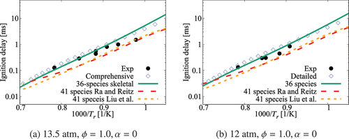
Figure 3. Comparison of ignition delay times calculated using the 36-species skeletal and high-$T$ part of the comprehensive (Zhang et al. 2016) mechanisms. Results for the skeletal mechanisms of Ra and Reitz (2008) and Liu et al. (2012) are also shown. Experimental data is from Gauthier, Davidson, and Hanson (2004) and Ciezki and Adomeit (1993)

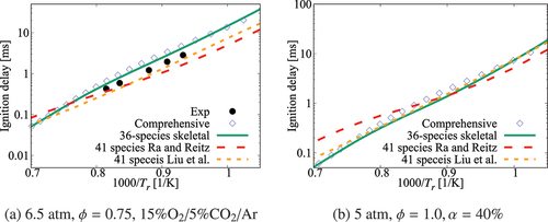
The measurement of $\tau$ for diluted mixture is scarce. Figure 4a compares the computed and measured values of $\tau$ for CO₂ diluted mixtures. All the mechanisms show some minor deviations from the measurements, however, the 36-species and Liu et al. (2012) mechanisms yield improved estimates. The values of $\tau$ obtained using the comprehensive mechanism are set as reference values for comparison shown in Figure 4b as there is no measurement available. The results of 36-species and Liu et al. (2012) mechanisms agree with estimates from the comprehensive mechanism over the temperature range of interest. The mechanism of Ra and Reitz (2008) shows large discrepancy for $1000/T_r\le 0.8$. Although the results in this figure are shown for $\alpha =40\mathrm{\%}$, this comparison is typical for diluted mixtures. Despite the lack of experimental data for diluted conditions, it is worth to comment that the 36-species mechanism along with the comprehensive mechanism perform uniformly better compared to the other two skeletal mechanisms for conditions tested in Figures 2-4. A weak non-linear behavior in the range $0.9<1000/T_r<1.0$ is observed for the non-diluted cases. However, for the diluted case shown in Figure 4a, the measurements suggest a linear behavior over this temperature range, which is captured well by the skeletal mechanisms.

Figure 4. Comparison of ignition delay times calculated using the 36-species skeletal and high-$T$ part of the comprehensive (Zhang et al. 2016) mechanisms along with those for the skeletal mechanisms of Ra and Reitz (2008) and Liu et al. (2012). Experimental data is from Campbell et al. (2015)

It is worth to note that the 41-species mechanisms of Ra and Reitz (2008) and Liu et al. (2012) were obtained using the comprehensive mechanism of Curran et al. (1998, 2002) with more than 550 species and 4500 reactions employing different reduction strategies as described in their papers. One may contemplate that the differences in autoignition delays computed using the 36-species and 41-species mechanisms shown in Figures 2-4 of the current study may come from the respective comprehensive mechanisms. This is tested in the Appendix and the results are shown in Figures A1 and A2. It is clear that these two comprehensive mechanisms yield almost the same ignition delay times which compare well with measurements. Thus, the differences seen in Figures 2-4 arise from the reduction strategies employed by Ra and Reitz (2008) and Liu et al. (2012).

Performance of the 36-species mechanism is tested further against the comprehensive mechanism for various values of pressure, $\varphi$ and $\alpha$. The results in Figures 5–7 show an excellent agreement for $1000/T_r\le 0.85$. Small differences appear for $1000/T_r>0.85$ which corresponds to $T_r<1176$ K. The typical errors for $1000/T_r>0.85$ are listed in Table 1 for 1, 5, and 10 atm, three equivalence ratios and four dilution levels. The absolute error values suggest a positive correlation with the dilution level at atmospheric pressure and for some specific conditions like 5 atm with $\varphi =1.0$ and 10 atm with an equivalence ratio of 0.95. However, it is difficult to generalize this observation since such a trend is not observed for other conditions listed in the Table. Overall, the error is observed to be below $30\mathrm{\%}$, which may be considered to be acceptable given that there are only 36 species while a typical comprehensive mechanism involves many 100s of species. Furthermore, the aim here is to get a skeletal mechanism which can be used in simulations of turbulent MILD combustion involving wide range of $\alpha$, $p$ and $\varphi$ values while capturing the trends in $\tau$ variations using as small number of species as possible.

Figure 5. Comparison of ignition delay times calculated using the 36-species skeletal (symbols) and comprehensive (lines) mechanisms for 1 atm and $\varphi =0.7$ $n$-heptane/air mixture with various dilution levels. Solid line and squares are for no dilution, dashed line and circles are for $20\mathrm{\%}$ dilution, dotted line and stars are for $40\mathrm{\%}$ dilution, dash-dotted line and triangles are for $50\mathrm{\%}$ dilution.

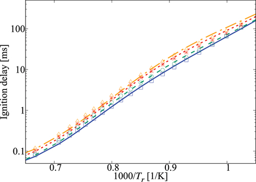
Figure 6. Comparison of ignition delay times calculated using the 36-species skeletal (symbols) and comprehensive (lines) mechanisms for 5 atm and $\varphi =1.6$ $n$-heptane/air mixture with various dilution levels. Solid line and squares are for no dilution, dashed line and circles are for $20\mathrm{\%}$ dilution, dotted line and stars are for $40\mathrm{\%}$ dilution, dash-dotted line and triangles are for $50\mathrm{\%}$ dilution.

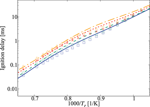
Figure 7. Comparison of ignition delay times calculated using the 36-species skeletal (symbols) and comprehensive (lines) mechanisms for 10 atm and $\varphi =1$ $n$-heptane/air mixture with various dilution levels. Solid line and squares are for no dilution, dashed line and circles are for $20\mathrm{\%}$ dilution, dotted line and stars are for $40\mathrm{\%}$ dilution, dash-dotted line and triangles are for $50\mathrm{\%}$ dilution.

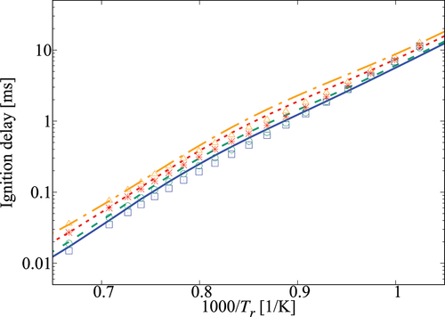
Table 1. Percentage error in $\tau$ computed using the 36-species skeletal mechanism in comparison to that obtained using the comprehensive mechanism.

Pressure	$\alpha$ ($\mathrm{\%}$)		error ($\mathrm{\%}$)
		$\varphi$ = 1.0	$\varphi$ = 0.95	$\varphi$ = 0.85
1 atm	0	+3.62	−3.02	−3.62
	20	−5.21	−10.11	−0.17
	40	−12.76	−13.25	+5.59
	50	−15.76	−13.18	+8.86
5 atm	0	+13.69	−4.84	−25.70
	20	+0.087	−16.94	−26.61
	40	−13.53	−27.46	−22.39
	50	−20.69	−31.90	−18.91
10 atm	0	+24.34	5.19	−20.55
	20	+11.57	5.95	−25.14
	40	−0.89	−16.65	−26.67
	50	−7.49	−21.76	−25.80

Reaction sensitivity analysis for $\tau$ using brute force method (Ji et al. 2015) is conducted and the normalized sensitivity coefficients are presented in Figure 8. The reactions with sensitivity coefficient of $\left|(\mathrm{\partial }ln\tau )/(\mathrm{\partial }lnk)\right|15\mathrm{\%}$ (rate constant $k$ is perturbed by 5 $\mathrm{\%}$) are shown in this figure for 1 and 10 atm. The comprehensive and skeletal mechanisms show similar reactions with top sensitivities. Regardless of dilution level, $\tau$ is most sensitive to the forward reaction of the chain branching step H + O₂ $\iff$ O + OH in the comprehensive mechanism for the atmospheric pressure. Additionally, the chain propagation reactions C₂H₄ + OH $\iff$ C₂H₃ + H₂O and CH₃ + HO₂ $\iff$ CH₃O + OH rank as the top three most sensitive reactions. All of them show negative sensitivity. The reaction with highest positive sensitivity (ranks as 4th or 5th if one uses sensitivity coefficient) is CH₃ + HO₂ $\iff$ CH₄ + O₂, which falls in the chain termination category.

Figure 8. Typical reaction sensitivity for ignition delay time at 1 and 10 atm with $T_r=1200\mathrm{K}$.

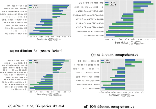
Similar conclusion can be drawn with minor difference on the absolute values of normalized sensitivity for the elevated pressure case. Additionally, several pyrolysis-related reactions show noticeable contribution for $T_r=1200\mathrm{K}$, for example, the parent fuel pyrolysis through H atom abstraction leading to C₇H₁₅ isomers: NC₇H₁₆ + OH $\iff$ C₇H₁₅-3 + H₂O, NC₇H₁₆ + H $\iff$ C₇H₁₅-3 + H₂ and an alternative route: NC₇H₁₆ $\iff$ NC₃H₇ + PC₄H₉. These reactions, except the alternative route, have higher sensitivity for $\tau$ at $T_r$ lower than 1000 K for the following reasons. The pyrolysis of $n$-heptane starts at about 750 K contributing to low-temperature ignition. Many of these pyrolysis reactions have either negative or zero activation energy implying that these reactions are low-temperature reactions and thus show higher sensitivity to $\tau$ for lower $T_r$, which may not be of interest to MILD combustion because $T_r$ is typically above 1100 K. At $T_r$ higher than 1300 K, their sensitivities are much lower – these are not shown here for brevity. The skeletal mechanism shows similar reaction sensitivity rankings and values which are comparable to those from the comprehensive mechanism for the range of conditions investigated. For the diluted case, the pressure dependent reaction C₂H₄ + H (+M) = C₂H₅(+M) does not appear in the list while it has a sensitivity coefficient of 0.5 for the undiluted case. More importantly, the sensitivity coefficient for C₂H₄ + OH = C₂H₃ + H₂O changes from −0.75 to −1.0, at 10 atm, for the diluted case because of the increased level of OH produced through diluent species H₂O.

Laminar flame speed comparisons

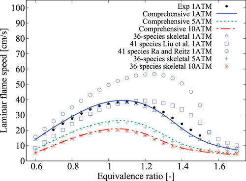
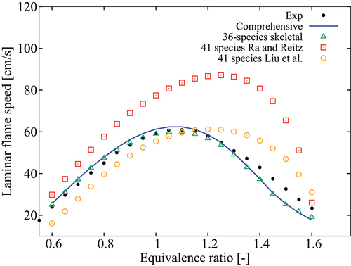
Figure 9 compares the measured and computed $S_L$ over a range of pressure for undiluted mixtures with $T_r=298$ K. The flame speeds are obtained from freely propagating, adiabatic, 1-D laminar flames computed using Cantera (Goodwin, Moffat, Speth 2017). Various chemical mechanisms are used for these calculations as noted in the figure. The experimental data of Dirrenberger et al. (2014) for 1 atm agrees well with those computed using the comprehensive and 36-species skeletal mechanisms. The 41-species skeletal mechanisms of Liu et al. (2012) and Ra and Reitz (2008) show some deviations. For 5 and 10 atm, $S_L$ computed using the 36-species mechanism agree well with those obtained from the comprehensive mechanism.

Figure 9. Comparison of laminar flame speeds computed using various mechanisms with measurement at 1/5/10 atm, $T_r=298$ K and $\alpha =0$.

Further validations of $S_L$ for undiluted $n$-heptane/air mixtures at different pressures and $T_r$ are presented in Figures 10–12. The 41-species mechanisms yield noticeably different flame speeds for all the cases whereas the 36-species mechanism yields a good agreement. It is worth noting that the 41-species mechanisms gave reasonable agreement for $\tau$ as discussed in Section 3.1 but they give substantially different flame speeds. This is because, these two mechanisms were developed for autoignition at high pressures relevant for IC engines. Furthermore, the $n$-heptane oxidation part in the mechanisms of Ra and Reitz (2008) and Liu et al. (2012) was based on the comprehensive mechanism of Curran et al. (1998, 2002) which was developed with interest to capture autoignition delay time variations. Hence, its ability to capture $S_L$ variations with equivalence ratio, $T_r$ and $p$ is studied in Figure A3 of the Appendix. Thus, the over estimate of $S_L$ by the two 41-species mechanisms is not surprising as it stems from the base comprehensive mechanism itself. Therefore, it is reasonable to conclude that the errors in $\tau$ and $S_L$ for the 41-species mechanisms are for different reasons – the reduction strategies employed in these previous studies contribute to the error in $\tau$ while the error in $S_L$ arises from the comprehensive mechanism itself. From these observations, it is quite clear that one must be careful while developing skeletal mechanism for MILD combustion since autoignition and flame propagation are equally important for this combustion.

Figure 10. Comparison of laminar flame speeds computed using various mechanisms with measurements of Dirrenberger et al. (2014) for 1 atm, $T_r=398$ K and $\alpha =0$.

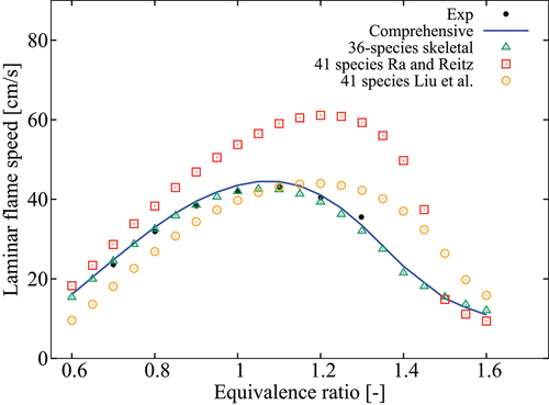
Figure 11. Comparison of computed laminar flame speeds with measurements from Kelley et al. (2011) for 2 atm, $T_r=353$ K and $\alpha =0$.

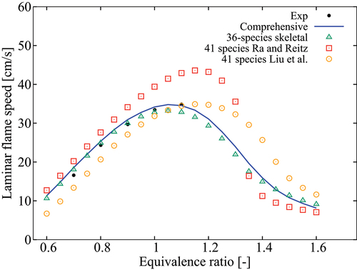
Figure 12. Comparison of computed laminar flame speeds with measurements from Kelley et al. (2011) for 5 atm, $T_r=353$ K and $\alpha =0$.

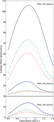
Typical comparisons for diluted mixtures are shown in Figure 13 and thus only three conditions are chosen for discussion here. Increased pressure or dilution level lead to lower $S_L$ while elevated $T_r$ result in faster flames. Satisfactory comparisons between values obtained using the 36-species and the comprehensive mechanisms are observed and there are some minor underestimates for mixtures with $1.0\le \varphi \le 1.3$. For richer mixtures, $\varphi \ge 1.50$, the 36-species skeletal mechanism over estimates $S_L$ by about $10-15\mathrm{\%}$ for most cases. The sensitivity analyses for $S_L$ using the brute force method of Ji et al. (2015) give results similar to those shown in Figure 10 and hence they are not shown here.

Figure 13. Comparison of laminar flame speeds obtained using 36-species skeletal (symbols) and comprehensive (lines) mechanisms. Solid line and squares are for 1 atm, dashed line and circles are for 5 atm, and dotted line and triangles are for 10 atm. The flame speed values for $T_r=700\mathrm{K}$ with $20\mathrm{\%}$ and $50\mathrm{\%}$ dilutions are shifted up by 20 cm/s for clarity.

The mechanism of Zhang et al. (2016) took about 720s to compute the laminar flame speed for strongly diluted ($\alpha =40\mathrm{\%}$) stoichiometric mixture at 5 atm and 930 K whereas the 36-species skeletal mechanism took about 9.5s. For ignition delay time calculations under strongly diluted conditions, there is about 8x speed up for the skeletal mechanism. Although these calculations take longer to converge for mixtures close to flammability limit the computational time difference between the skeletal and comprehensive mechanisms remains more or less the same as noted above.

Chemiluminescent species

Chemiluminescent species such as OH* and CH* can be useful in determining flame parameters such as stoichiometry and heat release (Kathrotia et al. 2012). The kinetic modeling of these species needs C, CH, and C₂H which are unavailable in the 36-species skeletal mechanism. The sub-mechanism for OH*, CH*, the above three and other required species can be simply added to the skeletal mechanism but this increases the total number of species substantially, from 36 to 67 species. This 67-species skeletal mechanism is obtained as an intermediate step, which brings practical challenges for turbulent MILD combustion simulations. Furthermore, the 31 additional species are short-lived and hence impose constrains on the time-stepping which will increase the computational burden substantially for 3D turbulent reacting flow simulations. Including these additional species will help with quantitative estimates of the chemiluminescent species concentration, which was verified but not shown here. However, identifying the spatial distribution of heat releasing regions, their morphologies and topologies are of high interest for turbulent simulations and hence a qualitative estimates of the levels of chemiluminescent species are adequate. For these reasons, QSSA is employed for 31 species which helps us to get 36-species skeletal mechanism and to estimate the chemiluminescent species concentration. The QSSA² relations are obtained using CARM outlined in Section 2. The accuracy of this approximation is tested by comparing the chemiluminescent species distribution obtained using the comprehensive mechanism and the QSSA. Typical results are shown in Figure 14 for three selected conditions: undiluted stoichiometric mixture at 5 atm, a lean mixture with 20% dilution at atmospheric pressure and a rich mixture with 50% dilution at 10 atm. The progress variable is defined as $c=\left(T-T_r\right)/\left(T_b-T_r\right)$, where $T_b$ is the burnt mixture temperature.

Figure 14. Comparison of OH* and CH* levels obtained using the comprehensive mechanism (solid lines) and QSSA with 36-species skeletal mechanism (dashed lines) for $T_r=353$ K.

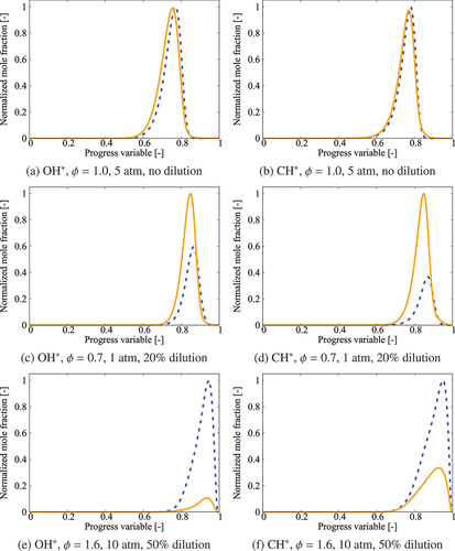
There are some differences in the OH* and CH* obtained using QSSA depending on the mixture condition. A good agreement is observed for mixtures with $\alpha 40\mathrm{\%}$; the maximum discrepancy in the peak value is about 150% for the results in Figure 14c. A relatively large difference, up to 8 times as in Figure 14e, is seen for $\varphi =0.7$ and 1.6 mixtures with high dilution whereas the agreement is good for the stoichiometric mixture. 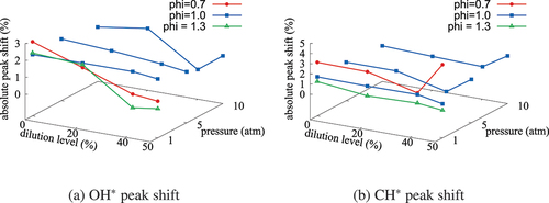Despite these quantitative differences, which are expected as noted earlier, the locations of peak levels in the $c$ and physical spaces agree well for the skeletal and comprehensive mechanisms as observed in Figure 15 which shows the absolute percentage shift in the location of the peak OH* and CH* for various pressure, $\varphi$ and $\alpha$ values. The shifts for OH* and CH* are below 5% and there seems to be a decreasing (increasing) trend in general with the dilution level (pressure). Hence, the QSSA approximation is good for qualitative estimates of OH* and CH* to satisfy the requirement for high fidelity simulations of turbulent MILD combustion.

Figure 15. The variations of absolute percentage difference in the locations of peak values of OH* and CH* computed using the skeletal and comprehensive mechanisms for various values of $\alpha$, $\varphi$, and $p$.

Application to turbulent MILD combustion

The combustion of pre-vaporized $n$-heptane injected into a hot co-flow with varying level of oxygen is simulated using URANS approach with a finite rate chemistry model and the 36-species skeletal mechanism as a first step to validate this mechanism for turbulent combustion simulations. The Jet in Hot Co-flow (JHC) burner shown schematically in Figure 16 was investigated experimentally and numerically in past studies (Li et al. 2021a; Ye et al. 2017). The fuel injected through a jet of diameter $D$ reacts with the hot co-flow at $1250\mathrm{K}$. 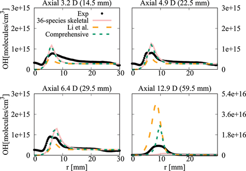The oxygen level in the co-flow is controlled to be at 3%, 6%, or 9% by volume. Measured temperature and OH number density, quantified using a method reported by Medwell, Kalt, and Dally (2007), at various axial locations of 14.5, 22.5, 29.5, and 59.5 mm are used to validate the computational results. URANS results of Li et al. (2021a) obtained with a chemical mechanism of Ranzi et al. (2014) and Stagni et al. (2014) involving 106 species and 1738 reactions are considered for comparative analysis.

Figure 16. Two-dimensional schematic for the computational domain with boundary conditions used for the JHC burner of Li et al. (2021a)

A two-dimensional axisymmetric structured mesh with about 4450 hexahedral and 100 prism cells is used for the simulations reported in this study. The computational domain includes about 100 mm long fuel central jet and hot co-flow annular jet upstream of the burner exit. The outlet of the computational domain is located at 100 mm from the burner exit. Medwell, Kalt, and Dally (2007) suggested that the influences of the coflow remain for about 100 mm downstream of the jet exit. Therefore, entrainment effects of the surrounding air are not considered in this study. The Partially Stirred Reactor (PaSR) combustion model with the dynamic calculation of mixing timescale (Li et al. 2018) is used along with the $k$-$\in$ turbulence model and Pope (1978) correction for round jet anomaly.

In the theory of PaSR combustion model (Chomiak 1990; Golovitchev and Chomiak 2001), each computational cell is split into two zones: one with reactions and another with mixing only. The averaged reaction rate in a cell is obtained as ${\bar{\dot{\omega }}}_i=\kappa \left(d{Y}_i^{\ast }/dt\right)$ with $\kappa ={\tau }_c/\left({\tau }_c+{\tau }_{mix}\right)$, where ${\tau }_c$ and ${\tau }_{mix}$ are respectively the characteristic chemical and mixing time scales in each computational cell. The mixing time scale is estimated as the ratio of Favre variance of the mixture fraction, $Z^2$, to its dissipation rate, ${\in }_Z$, and these quantities are obtained using their respective transport equations as by Li et al. (2018). Following Chomiak and Karlsson (1996) and Li et al. (2017b), (2018), the maximum of the ratio of species mass fraction to its reaction rate is used as the chemical timescale, ${\tau }_c=max\left({\tau }_{c,i}\right)=max\left(Y_i^{\ast }/\left|d{Y}_i^{\ast }/dt\right|\right)$,³ with $d{Y}_i^{\ast }/dt$ obtained using a canonical reactor.

The measured bulk-mean axial velocity and temperature in the respective streams are listed in Table 2 which are used to specify the inlet conditions having radially uniform profiles. The Reynolds number is calculated based on the above velocity, hydraulic diameter and the mixture viscosity at the corresponding temperature. The equilibrium mass fractions for the inlet temperatures in Table 2 are used to specify the species inlet conditions. Further modeling details are discussed in Li et al. (2021a).

Table 2. Jet and coflow characteristics.

Quantities	Central jet	Hot coflow
Velocity	$50\mathrm{m}/\mathrm{s}$	$2.4\mathrm{m}/\mathrm{s}$
Temperature	$412\mathrm{K}$	$1250\mathrm{K}$
Reynolds number	10,000	1000

Figures 17–22 compare the radial variation of mean temperature and OH number density at four axial positions for the cases with $3\mathrm{\%}$, $6\mathrm{\%}$, and $9\mathrm{\%}$ oxygen by volume in the co-flow. Note that the experimental data for the $3\mathrm{\%}$ and $6\mathrm{\%}$ cases are not available for $4.9D$ axial position. The uncertainty for OH number density is the principle source of uncertainty for the Rayleigh scattering and can be estimated to be smaller than 2 $\mathrm{\%}$ (Sutton, Williams, Fleming 2008). The typical uncertainty in the temperature data in the coflow and reaction zone varies from 5% to 10 $\mathrm{\%}$ (Gordon, Masri, Mastorakos 2008; Medwell 2007; Ye et al. 2018). For the $3\mathrm{\%}$ case, the mean temperature computed in this study using the comprehensive and 36-species mechanisms agree well with measurements and the results of Li et al. (2021a). There are some differences for OH number density as seen in Figure 18 and the peak value at $12.9D$ obtained using the 36-species mechanism is closer to the measured value compared to those from the earlier study. For the $6\mathrm{\%}$ oxygen case shown in Figures 19 and 20, the mean temperature is under estimated slightly (about $40\mathrm{K}$) for all the computational results at the axial location of $12.9D$, which is within the uncertainty range for temperature. The OH number density is generally over estimated by the comprehensive and 36-species mechanisms for all axial positions except $12.9D$. The peak value is under estimated by the 36-species mechanism for $12.9D$ and the other cases compare quite well with the measurements. However, the location of the peak value is shifted toward the outer side of the jet as seen in Figure 20. Similar observations are made from Figures 21 and 22 shown for the case with $9\mathrm{\%}$ oxygen. Compared to the mechanism used by Li et al. (2021a), the peak value of OH number density computed in this study is closer to the measurement for $12.9D$ location. Regarding the radial variations of mean temperature, differences appear mainly at $12.9D$ location, where the mechanism used by Li et al. (2021a) yield values closer to the measurements. The comprehensive and 36-species mechanisms underestimate the peak mean temperature by about $100\mathrm{K}$, staying within the uncertainty range. The discrepancies between different simulation results observed for the 6% and 9% cases are likely due to the differences in the fuel pyrolysis reactions included in the mechanisms used. Even though several $n$-heptane pyrolysis-related species and reactions, such as NC₇H₁₆ $\iff$ PC₄H₉ + NC₃H₇, NC₇H₁₆ $\iff$ C₇H₁₅ + H and PC₄H₉ $\iff$ C₂H₄ + C₂H₅ are included in the 36-species mechanism, the lack of low-temperature mechanism results in insufficient modeling of the full fuel pyrolysis for cases with higher co-flow oxygen level of $6\mathrm{\%}$ and $9\mathrm{\%}$. Moreover, the mechanism used by Li et al. (2021a) was based on the comprehensive mechanism of Ranzi et al. (2012). This comprehensive mechanism is different from the one used for the current study. Hence, this can be another source for the differences in the computed values. Comparisons of $\tau$ and $S_L$ computed using these two comprehensive mechanisms for the conditions of turbulent flames show some notable differences (see Figures A4‒A6 in the Appendix), supporting the above point. It is clear that the 36-species mechanism obtained in this study gives improved results for the most diluted cases with 3% oxygen since this mechanism is developed specifically for diluted combustion under MILD conditions. It is also worth noting that the combustion is less likely to be MILD when the oxygen level is larger than 5% by volume (Li et al. 2021a; Ye et al. 2017). Furthermore, the CPU time taken for the simulations with 36-species mechanism is nearly 1/4th of that required for the mechanism used by Li et al. (2021a). The comprehensive mechanism of Zhang et al. (2016) took 18 times longer compared to the 36-species mechanism. These are substantial savings in computational cost to achieve the same level of predictive accuracy for MILD combustion.

Figure 17. Comparison of computed and measured mean temperature variations at four axial locations. Coflow oxygen level is 3%. The results of Li et al. (2021a) are also shown for comparison.

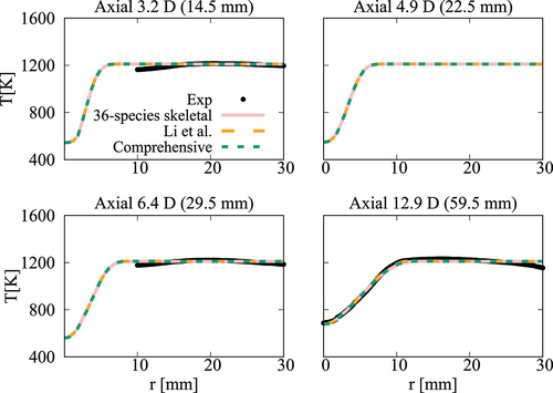
Figure 18. Comparison of computed and measured mean number density of OH at four axial locations. Coflow oxygen level is 3%. The results of Li et al. (2021a) are shown for comparison.

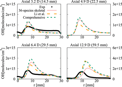
Figure 19. Comparison of computed and measured mean temperature variations at four axial locations. Coflow oxygen level is 6%. The results of Li et al. (2021a) are also shown for comparison.

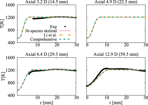
Figure 20. Comparison of computed and measured mean number density of OH at four axial locations. Coflow oxygen level is 6%. The results of Li et al. (2021a) are shown for comparison.

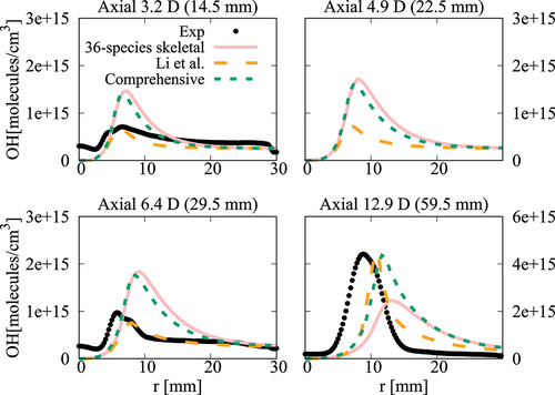
Figure 21. Comparison of computed and measured mean temperature variations at four axial locations. Coflow oxygen level is 6%. The results of Li et al. (2021a) are also shown for comparison.

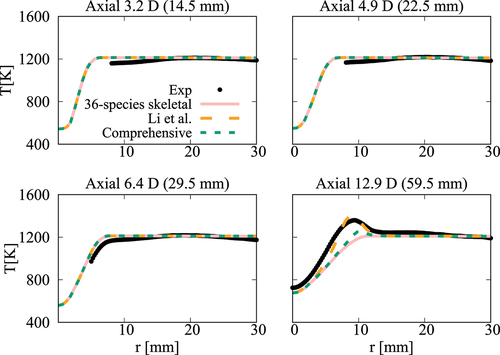
Figure 22. Comparison of computed and measured mean number density of OH at four axial locations. Coflow oxygen level is 9%. The results of Li et al. (2021a) are shown for comparison.

Conclusions

The Computer Assisted Reduction Mechanism approach is used to develop a $n$-heptane skeletal mechanism with 36 species and 205 reactions so that it can be employed for high fidelity simulations of MILD combustion using DNS and LES paradigms with direct chemistry integration. This mechanism is validated using ignition delay times, $\tau$, and laminar flame speeds, $S_L$, measured for representative conditions and the values of these two quantities computed using a comprehensive mechanism over wide ranges of pressure, mixture temperature, equivalence ratio and dilution level which are of interest for MILD combustion. These two characteristic quantities calculated using the 36-species mechanism is observed to agree well with measurements and those obtained using the comprehensive mechanism. Since MILD combustion typically involve reactant mixtures with temperature above $1100\mathrm{K}$, the skeletal mechanism does not involve elementary reactions relevant for NTC behavior of $n$-heptane/air mixtures and thus excludes LTC regime. However, this regime can be important for High Temperature Air Combustion.

Two existing skeletal mechanisms of Liu et al. (2012) and Ra and Reitz (2008) with 41 species are also tested for MILD combustion conditions. Although reasonable agreement for $\tau$ is observed in comparison to available measurements some deviations are noted for $S_L$. The errors on $S_L$ yielded by Ra et al.’s 41-species mechanism come from its starting mechanism. While the error for $\tau$ comes from the reduction strategies employed by Ra and Reitz (2008) because the $\tau$ computed using their starting mechanism and the comprehensive mechanism employed for the current study compare well. The chemiluminescent species, $\mathrm{O}{\mathrm{H}}^{\ast }$ and $\mathrm{C}{\mathrm{H}}^{\ast }$, obtained using quasi steady state approximation involving species in 36-species mechanism show satisfactory agreement with those computed using the comprehensive $n$-heptane/air mechanism with additional reactions for $\mathrm{O}{\mathrm{H}}^{\ast }$ and $\mathrm{C}{\mathrm{H}}^{\ast }$ chemistry.

URANS simulations of MILD combustion in jet in hot co-flow burner is conducted using finte rate chemistry models and the 36-species mechanism to assess the usability of this mechanism for turbulent MILD combustion simulations. The results demonstrate the suitability of this skeletal mechanism for these simulations and also show that the same level of accuracy can be achieved with substantially lower computation cost. Unfortunately, there are no $\mathrm{O}{\mathrm{H}}^{\ast }$ or $\mathrm{C}{\mathrm{H}}^{\ast }$ images available for comparisons. Simulations using DNS and LES paradigms are to be conducted to further test this mechanism. The distinct features shown by complex fuel under MILD regime in turbulent flows can be further explored by means of DNS and insights gathered thereby can be leveraged for industrial applications.

Acknowledgments

The support of EPSRC through the grant numbered EP/S025650/1 is gratefully acknowledged.

Disclosure statement

The authours declare that they have no known competing financial interests or personal relationships that could have appeared to influence the work reported in this paper.

Additional information

Funding

This work was supported by the Engineering and Physical Sciences Research Council [EP/S025650/1].

Notes

¹ A copy of CHEMKIN compatible files for this mechanism can be obtained by contacting the corresponding author.

² The QSSA post-processing tool can be obtained by contacting the corresponding author.

³ There is a minimum threshold value (10 ${ }^{-16}{s}^{-1}$) applied on $\left|d{Y}_i^{\ast }/dt\right|$ to eliminate dormant species.

Appendix A

Performance comparisons for comprehensive mechanisms of Zhang et al. (2016) and Curran et al. (1998, 2002)

Figure A1. Comparison of ignition delay times calculated using comprehensive mechanisms from Zhang et al. (2016) and Curran et al. (1998, 2002) for cases without dilution.

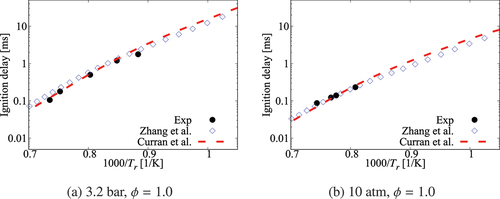
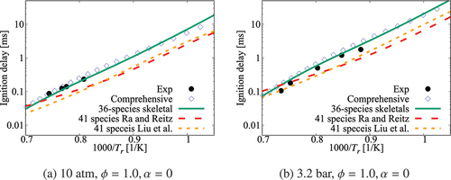
Figure A2. Comparison of ignition delay times calculated using comprehensive mechanisms from Zhang et al. (2016) and Curran et al. (1998, 2002) for case under 6.5 atm, $\varphi =0.75$, mixture composition n-heptane/15%O₂/5%CO₂/Ar.

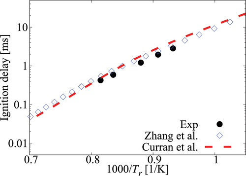
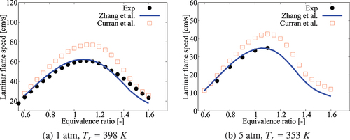
Figure A3. Comparison of laminar flame speeds calculated using comprehensive mechanisms from Zhang et al. (2016) and Curran et al. (1998, 2002) for cases without dilution.

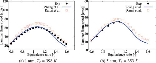
Performance comparisons for comprehensive mechanisms of Zhang et al. (2016) and Ranzi et al. (2012)

Figure A4. Comparison of ignition delay times calculated using comprehensive mechanisms from Zhang et al. and Ranzi et al. for cases without dilution.

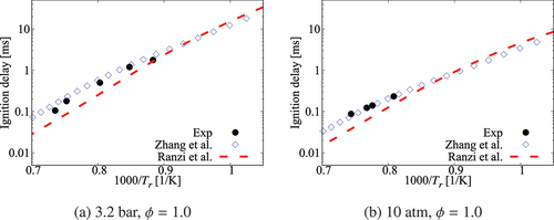
Figure A5. Comparison of ignition delay times calculated using comprehensive mechanisms from Zhang et al. and Ranzi et al. for case under 6.5 atm, $\varphi =0.75$, mixture composition n-heptane/15%O₂/5%CO₂/Ar.

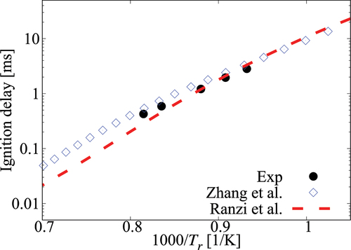
Figure A6. Comparison of laminar flame speeds calculated using comprehensive mechanisms from Zhang et al. and Ranzi et al. for cases without dilution.

References

- Arghode, V. K., and A. K. Gupta. 2010. Effect of flow field for colorless distributed combustion (CDC) for gas turbine combustion. Appl. Energy 87 (5):1631–40. doi:10.1016/j.apenergy.2009.09.032.
- Arghode, V. K., A. K. Gupta, and K. M. Bryden. 2012. High intensity colorless distributed combustion for ultra low emissions and enhanced performance. Appl. Energy 92:822–30. doi:10.1016/j.apenergy.2011.08.039.
- Bhaya, R., A. De, and R. Yadav. 2014. Large eddy simulation of MILD combustion using PDF-based turbulence-chemistry interaction models. Combust. Sci. Technol 186 (9):1138–65. doi:10.1080/00102202.2014.916702.
- Campbell, M. F., S. I. Wang, C. S. Goldenstein, R. M. Spearrin, A. M. Tulgestke, L. T. Zaczek, D. F. Davidson, and R. K. Hanson. 2015. Constrained reaction volume shock tube study of n-heptane oxidation: Ignition delay times and time-histories of multiple species and temperature. Proc. Combust. Inst 35 (1):231–39. doi:10.1016/j.proci.2014.05.001.
- Cavaliere, A., and M. de Joannon. 2004. MILD combustion. Prog. Energy Combust. Sci 30 (4):329–66. doi:10.1016/j.pecs.2004.02.003.
- Chen, J.-Y. 1988. A general procedure for constructing reduced reaction mechanisms with given independent relations. Combust. Sci. Technol 57 (1–3):89–94. doi:10.1080/00102208808923945.
- Chen, J.-Y. 2001. Automatic generation of reduced mechanisms and their applications to combustion modeling. Zhongguo Hangkong Taikong Xuehui Huikan 33 (2):59–67.
- Chen, J.-Y., and Y. F. Tham. 2008. Speedy solution of quasi-steady-state species by combination of fixed-point iteration and matrix inversion. Combust. Flame 153 (4):634–46. doi:10.1016/j.combustflame.2007.12.006.
- Chen, D., K. Wang, and H. Wang. 2017a . Violation of collision limit in recently published reaction models. Combust. Flame 186:208–10. doi:10.1016/j.combustflame.2017.08.005.
- Chen, Y., B. Wolk, M. Mehl, W. K. Cheng, J.-Y. Chen, and R. W. Dibble. 2017b. Development of a reduced chemical mechanism targeted for a 5-component gasoline surrogate: A case study on the heat release nature in a GCI engine. Combust. Flame 178:268–76. doi:10.1016/j.combustflame.2016.12.018.
- Chen, Y., and J.-Y. Chen. 2018. Towards improved automatic chemical kinetic model reduction regarding ignition delays and flame speeds. Combust. Flame 190:293–301. doi:10.1016/j.combustflame.2017.11.024.
- Chinnici, A., Z. F. Tian, J. H. Lim, G. J. Nathan, and B. B. Dally. 2017. Comparison of system performance in a hybrid solar receiver combustor operating with MILD and conventional combustion. Part II: Effect of the combustion mode. Sol. Energy 147:478–88.
- Chomiak, J. 1990. Combustion: A study in theory, fact and application. USA: Abacus Press/Gorden and Breach Science Publishers.
- Chomiak, J., and A. Karlsson. 1996. Flame liftoff in diesel sprays. Twenty-sixth symposium (International) on Combustion, Naples, Italy, 2557–64. The Combustion Institute.
- Ciezki, H. K., and G. Adomeit. 1993. Shock-tube investigation of self-ignition of n-heptane-air mixtures under engine relevant conditions. Combust. Flame 93 (4):421–33. doi:10.1016/0010-2180(93)90142-P.
- Cuoci, A., A. Frassoldati, T. Faravelli, and E. Ranzi. 2015. Opensmoke++: An object-oriented framework for the numerical modeling of reactive systems with detailed kinetic mechanisms. Comput. Phys. Commun. 192:237–64. doi:10.1016/j.cpc.2015.02.014.
- Curran, H. J., P. Gaffuri, W. J. Pitz, and C. K. Westbrook. 1998. A comprehensive modeling study of n-heptane oxidation. Combust. Flame 114 (1):149–77. doi:10.1016/S0010-2180(97)00282-4.
- Curran, H. J., P. Gaffuri, W. J. Pitz, and C. K. Westbrook. 2002. A comprehensive modeling study of iso-octane oxidation. Combust. Flame 129 (3):253–80. doi:10.1016/S0010-2180(01)00373-X.
- Dally, B. B., A. N. Karpetis, and R. S. Barlow. 2002. Structure of turbulent non-premixed jet flames in a diluted hot coflow. Proc. Combust. Inst 29 (1):1147–54. doi:10.1016/S1540-7489(02)80145-6.
- De, A., E. Oldenhof, P. Sathiah, and D. Roekaerts. 2011. Numerical simulation of Delft-Jet-in-Hot-Coflow (DJHC) flames using the Eddy dissipation concept model for turbulence-chemistry interaction. Flow Turbul. Combust. 87 (4):537–67. doi:10.1007/s10494-011-9337-0.
- de Joannon, M., P. Sabia, G. Sorrentino, and A. Cavaliere. 2009. Numerical study of MILD combustion in hot diluted diffusion ignition (HDDI) regime. Proc. Combust. Inst 32 (2):3147–54. doi:10.1016/j.proci.2008.09.003.
- de Joannon, M., G. Sorrentino, and A. Cavaliere. 2012. MILD combustion in diffusion-controlled regimes of hot diluted fuel. Combust. Flame 159 (5):1832–39. doi:10.1016/j.combustflame.2012.01.013.
- Dirrenberger, P., P. A. Glaude, R. Bounaceur, H. Le Gall, A. P. da Cruz, A. A. Konnov, and F. Battin-Leclerc. 2014. Laminar burning velocity of gasolines with addition of ethanol. Fuel 115:162–69. doi:10.1016/j.fuel.2013.07.015.
- Doan, A. K. N., and N. Swaminathan. 2019a . Autoignition and flame propagation in non-premixed MILD combustion. Combust. Flame 201:234–43. doi:10.1016/j.combustflame.2018.12.025.
- Doan, N. A. K., and N. Swaminathan. 2019b . Role of radicals on MILD combustion inception. Proc. Combust. Inst 37 (4):4539–46. doi:10.1016/j.proci.2018.07.038.
- Galletti, C., A. Parente, and L. Tognotti. 2007. Numerical and experimental investigation of a MILD combustion burner. Combust. Flame 151 (4):649–64. doi:10.1016/j.combustflame.2007.07.016.
- Gauthier, B. M., D. F. Davidson, and R. K. Hanson. 2004. Shock tube determination of ignition delay times in full-blend and surrogate fuel mixtures. Combust. Flame 139 (4):300–11. doi:10.1016/j.combustflame.2004.08.015.
- Golovitchev, V., and J. Chomiak. 2001. Numerical modeling of high temperature air flameless combustion. The 4th international symposium on high temperature air combustion and gasification, Rome, Italy, 27–30.
- Goodwin, D. G., H. K. Moffat, and R. L. Speth. 2017. Cantera: An object-oriented software toolkit for chemical kinetics, thermodynamics, and transport processes. Version 2.3.0. http://www.cantera.org.
- Gordon, R. L., A. R. Masri, and E. Mastorakos. 2008. Simultaneous Rayleigh temperature, OH- and CH2O-LIF imaging of methane jets in a vitiated coflow. Combust. Flame 155 (1–2):181–95. doi:10.1016/j.combustflame.2008.07.001.
- Graça, M., A. Duarte, P. J. Coelho, and M. Costa 2013. Numerical simulation of a reversed flow small-scale combustor. Fuel Proc. Technol., 107, 126–37.
- Ji, W., P. Zhang, T. He, Z. Wang, L. Tao, X. He, and C. K. Law. 2015. Intermediate species measurement during iso-butanol auto-ignition. Combust. Flame 162 (10):3541–53. doi:10.1016/j.combustflame.2015.06.010.
- Ju, Y. 2021. Understanding cool flames and warm flames. Proc. Combust. Inst 38 (1):83–119. doi:10.1016/j.proci.2020.09.019.
- Karyeyen, S., J. S. Feser, and A. K. Gupta. 2019. Hydrogen concentration effects on swirl-stabilized oxy-colorless distributed combustion. Fuel 253:772–80. doi:10.1016/j.fuel.2019.05.008.
- Kathrotia, T., U. Riedel, A. Seipel, K. Moshammer, and A. Brockhinke. 2012. Experimental and numerical study of chemiluminescent species in low-pressure flames. Appl. Phys. B 107 (3):571–84. doi:10.1007/s00340-012-5002-0.
- Katsuki, M., and T. Hasegawa. 1998. The science and technology of combustion in highly preheated air. Symp. (Int.) Combust 27 (2):3135–46. doi:10.1016/S0082-0784(98)80176-8.
- Kelley, A. P., A. J. Smallbone, D. L. Zhu, and C. K. Law. 2011. Laminar flame speeds of C5 to C8 n-alkanes at elevated pressures: Experimental determination, fuel similarity, and stretch sensitivity. Proc. Combust. Inst 33 (1):963–70. doi:10.1016/j.proci.2010.06.074.
- Khalil, A. E. E., and A. K. Gupta. 2014. Swirling flowfield for colorless distributed combustion. Appl. Energy 113:208–18. doi:10.1016/j.apenergy.2013.07.029.
- Khalil, A. E. E., and A. K. Gupta. 2015. Impact of pressure on high intensity colorless distributed combustion. Fuel 143:334–42. doi:10.1016/j.fuel.2014.11.061.
- Khalil, A. E. E., and A. K. Gupta. 2017. Towards colorless distributed combustion regime. Fuel 195:113–22. doi:10.1016/j.fuel.2016.12.093.
- Kruse, S., B. Kerschgens, L. Berger, E. Varea, and H. Pitsch. 2015. Experimental and numerical study of MILD combustion for gas turbine applications. Appl. Energy 148:456–65. doi:10.1016/j.apenergy.2015.03.054.
- Li, Y., C.-W. Zhou, K. P. Somers, K. Zhang, and H. J. Curran. 2017a . The oxidation of 2-butene: A high pressure ignition delay, kinetic modeling study and reactivity comparison with isobutene and 1-butene. Proc. Combust. Inst 36 (1):403–11. doi:10.1016/j.proci.2016.05.052.
- Li, Z., A. Cuoci, A. Sadiki, and A. Parente. 2017b. Comprehensive numerical study of the Adelaide Jet in Hot-Coflow burner by means of RANS and detailed chemistry. Energy 139:555–70. doi:10.1016/j.energy.2017.07.132.
- Li, Z., M. Ferrarotti, A. Cuoci, and A. Parente. 2018. Finite-rate chemistry modelling of non-conventional combustion regimes using a partially-stirred reactor closure: Combustion model formulation and implementation details. Appl. Energy 225:637–55. doi:10.1016/j.apenergy.2018.04.085.
- Li, Z., A. Cuoci, and A. Parente. 2019. Large eddy simulation of MILD combustion using finite rate chemistry: Effect of combustion sub-grid closure. Proc. Combust. Inst 37 (4):4519–29. doi:10.1016/j.proci.2018.09.033.
- Li, Z., M. J. Evans, J. Ye, P. R. Medwell, and A. Parente. 2021a. Numerical and experimental investigation of turbulent n-heptane jet-in-hot-coflow flames. Fuel 283:118748. doi:10.1016/j.fuel.2020.118748.
- Li, Z., S. Tomasch, Z. X. Chen, A. Parente, I. S. Ertesvåg, and N. Swaminathan. 2021b. Study of MILD combustion using LES and advanced analysis tools. Proc. Combust. Inst 38 (4):5423–32. doi:10.1016/j.proci.2020.06.298.
- Liu, Y.-D., M. Jia, M.-Z. Xie, and B. Pang. 2012. Enhancement on a skeletal kinetic model for primary reference fuel oxidation by using a semidecoupling methodology. Energy & Fuels 26 (12):7069–83. doi:10.1021/ef301242b.
- Lu, T., and C. K. Law. 2008. Strategies for mechanism reduction for large hydrocarbons: N-heptane. Combust. Flame 154 (1):153–63. doi:10.1016/j.combustflame.2007.11.013.
- Medwell, P. R. 2007. Laser diagnostics in MILD combustion. Phd thesis, University of Adelaide, Adelaide, Australia.
- Medwell, P. R., P. A. M. Kalt, and B. B. Dally. 2007. Simultaneous imaging of OH, formaldehyde, and temperature of turbulent nonpremixed jet flames in a heated and diluted coflow. Combust. Flame 148 (1):48–61. doi:10.1016/j.combustflame.2006.10.002.
- Medwell, P. R., and B. B. Dally. 2012. Effect of fuel composition on jet flames in a heated and diluted oxidant stream. Combust. Flame 159 (10):3138–45. doi:10.1016/j.combustflame.2012.04.012.
- Mehl, M., W. J. Pitz, C. K. Westbrook, and H. J. Curran. 2011. Kinetic modeling of gasoline surrogate components and mixtures under engine conditions. Proc. Combust. Inst 33 (1):193–200. doi:10.1016/j.proci.2010.05.027.
- Minamoto, Y., N. Swaminathan, R. S. Cant, and T. Leung. 2014. Reaction zones and their structure in MILD combustion. Combust. Sci. Technol 186 (8):1075–96. doi:10.1080/00102202.2014.902814.
- Minamoto, Y., and N. Swaminathan. 2014. Scalar gradient behaviour in MILD combustion. Combust. Flame 161 (4):1063–75. doi:10.1016/j.combustflame.2013.10.005.
- Niemeyer, K. E., and C.-J. Sung. 2011. On the importance of graph search algorithms for drgep-based mechanism reduction methods. Combust. Flame 158 (8):1439–43. doi:10.1016/j.combustflame.2010.12.010.
- Parente, A., C. Galletti, and L. Tognotti. 2008. Effect of the combustion model and kinetic mechanism on the MILD combustion in an industrial burner fed with hydrogen enriched fuels. Int. J. Hydrogen Energy 33 (24):7553–64. doi:10.1016/j.ijhydene.2008.09.058.
- Pelucchi, M., M. Bissoli, C. Cavallotti, A. Cuoci, T. Faravelli, A. Frassoldati, E. Ranzi, and A. Stagni. 2014. Improved kinetic model of the low-temperature oxidation of n -heptane. Energy & Fuel 28 (11):7178–93. doi:10.1021/ef501483f.
- Pepiot-Desjardins, P., and H. G. Pitsch. 2008. An efficient error-propagation-based reduction method for large chemical kinetic mechanisms. Combust. Flame 154 (1):67–81. doi:10.1016/j.combustflame.2007.10.020.
- Perpignan, A. V., A. G. Rao, and D. J. E. M. Roekaerts. 2018. Flameless combustion and its potential towards gas turbines. Prog. Energy Combust. Sci 69:28–62. doi:10.1016/j.pecs.2018.06.002.
- Pope, S. B. 1978. An explanation of the turbulent round-jet/plane-jet anomaly. Aiaa 16 (3):279–81. doi:10.2514/3.7521.
- Ra, Y., and R. D. Reitz. 2008. A reduced chemical kinetic model for IC engine combustion simulations with primary reference fuels. Combust. Flame 155 (4):713–38. doi:10.1016/j.combustflame.2008.05.002.
- Ranzi, E., A. Frassoldati, R. Grana, A. Cuoci, T. Faravelli, A. P. Kelley, and C. K. Law. 2012. Hierarchical and comparative kinetic modeling of laminar flame speeds of hydrocarbon and oxygenated fuels. Prog. Energy Combust. Sci 38 (4):468–501. doi:10.1016/j.pecs.2012.03.004.
- Ranzi, E., A. Frassoldati, A. Stagni, M. Pelucchi, A. Cuoci, and T. Faravelli. 2014. Reduced kinetic schemes of complex reaction systems: Fossil and biomass-derived transportation fuels. Int. J. Chem. Kinetics 46 (9):512–42. doi:10.1002/kin.20867.
- Reddy, V. M., P. Biswas, P. Garg, and S. Kumar. 2014. Combustion characteristics of biodiesel fuel in high recirculation conditions. Fuel Proc. Techno.l 118:310–17. doi:10.1016/j.fuproc.2013.10.004.
- Saha, M., B. B. Dally, P. R. Medwell, and E. M. Cleary. 2014. Moderate or Intense Low oxygen Dilution (MILD) combustion characteristics of pulverized coal in a self-recuperative furnace. Energy & Fuels 28 (9):6046–57. doi:10.1021/ef5006836.
- Seidel, L., K. Moshammer, X. Wang, T. Zeuch, K. Köhse-HÃinghaus, and F. Mauss. 2015. Comprehensive kinetic modeling and experimental study of a fuel-rich, premixed n-heptane flame. Combust. Flame 162 (5):2045–58. doi:10.1016/j.combustflame.2015.01.002.
- Shen, H.-P. S., J. Steinberg, J. Vanderover, and M. A. Oehlschlaeger. 2009. A shock tube study of the ignition of n-heptane, n-decane, n-dodecane, and n-tetradecane at elevated pressures. Energy & Fuels 23 (5):2482–89. doi:10.1021/ef8011036.
- Sorrentino, G., P. Sabia, M. de Joannon, A. Cavaliere, and R. Ragucci. 2016. The effect of diluent on the sustainability of mild combustion in a cyclonic burner. Flow Turbul. Combust. 96 (2):449–68. doi:10.1007/s10494-015-9668-3.
- Sorrentino, G., P. Sabia, P. Bozza, R. Ragucci, and M. de Joannon. 2019. Low-nox conversion of pure ammonia in a cyclonic burner under locally diluted and preheated conditions. Appl. Energy 254:113676. doi:10.1016/j.apenergy.2019.113676.
- Stagni, A., A. Cuoci, A. Frassoldati, T. Faravelli, and E. Ranzi. 2014. Lumping and reduction of detailed kinetic schemes: An effective coupling. Ind. Eng. Chem. Res. 53 (22):9004–16. doi:10.1021/ie403272f.
- Sutton, J. A., B. A. Williams, and J. W. Fleming. 2008. Laser-induced fluorescence measurements of NCN in low-pressure CH4/O2/N2 flames and its role in prompt NO formation. Combust. Flame 153 (3):465–78. doi:10.1016/j.combustflame.2007.09.008.
- Tham, Y. F., F. Bisetti, and J.-Y. Chen. 2008. Development of a highly reduced mechanism for iso-octane HCCI combustion with targeted search algorithm. J. Eng. Gas Turbines Power 130 (4):042804. doi:10.1115/1.2900729.
- Veríssimo, A. S., A. M. A. Rocha, and M. Costa. 2011. Operational, combustion, and emission characteristics of a small-scale combustor. Energy & Fuels 25 (6):2469–80. doi:10.1021/ef200258t.
- Wang, H., M. Yao, and R. D. Reitz. 2013. Development of a reduced primary reference fuel mechanism for internal combustion engine combustion simulations. Energy & Fuels 27 (12):7843–53. doi:10.1021/ef401992e.
- Weber, R., J. P. Smart, and W. vd Kamp. 2005. On the (MILD) combustion of gaseous, liquid, and solid fuels in high temperature preheated air. Proc. Combust. Inst 30 (2):2623–29. doi:10.1016/j.proci.2004.08.101.
- Weber, R., A. K. Gupta, and S. Mochida. 2020. High temperature air combustion (HiTAC): How it all started for applications in industrial furnaces and future prospects. Appl. Energy 278:115551. doi:10.1016/j.apenergy.2020.115551.
- Wünning, J. A., and J. G. Wünning. 1997. Flameless oxidation to reduce thermal NO-formation. Prog. Energy Combust. Sci 23 (1):81–94. doi:10.1016/S0360-1285(97)00006-3.
- Ye, J., P. R. Medwell, E. Varea, S. Kruse, B. B. Dally, and H. G. Pitsch. 2015. An experimental study on MILD combustion of prevaporised liquid fuels. Appl. Energy 151:93–101. doi:10.1016/j.apenergy.2015.04.019.
- Ye, J., P. R. Medwell, M. J. Evans, and B. B. Dally. 2017. Characteristics of turbulent n-heptane jet flames in a hot and diluted coflow. Combust. Flame 183:330–42. doi:10.1016/j.combustflame.2017.05.027.
- Ye, J., P. R. Medwell, K. Kleinheinz, M. J. Evans, B. B. Dally, and H. G. Pitsch. 2018. Structural differences of ethanol and DME jet flames in a hot diluted coflow. Combust. Flame 192:473–94. doi:10.1016/j.combustflame.2018.02.025.
- Yoo, C. S., T. Lu, J. H. Chen, and C. K. Law. 2011. Direct numerical simulations of ignition of a lean n-heptane/air mixture with temperature inhomogeneities at constant volume: Parametric study. Combust. Flame 158 (9):1727–41. doi:10.1016/j.combustflame.2011.01.025.
- Zhang, K., C. Banyon, J. Bugler, H. J. Curran, A. Rodriguez, O. Herbinet, F. Battin-Leclerc, C. B’Chir, and K. A. Heufer. 2016. An updated experimental and kinetic modeling study of n-heptane oxidation. Combust. Flame 172:116–35. doi:10.1016/j.combustflame.2016.06.028.
- Zhen, X., Y. Wang, and D. Liu. 2016. A new improvement on a chemical kinetic model of primary reference fuel for multi-dimensional CFD simulation. Energy Convers. Manage. 109:113–21. doi:10.1016/j.enconman.2015.11.061.
- Zhou, C.-W., Y. Li, E. O’Connor, K. P. Somers, S. Thion, C. Keesee, O. Mathieu, E. L. Petersen, T. A. DeVerter, M. A. Oehlschlaeger, et al. 2016. A comprehensive experimental and modeling study of isobutene oxidation. Combust. Flame 167:353–79. doi:10.1016/j.combustflame.2016.01.021.