Characterization of Flame Spread Over PMMA Using a Temperature Reconstruction Method

ABSTRACT

The contribution of heat transfer mechanisms for different configurations of opposed flow flame spread on cast PMMA is presented. Three opposed flow flame spread scenarios are considered, each in a quiescent atmosphere: downward spread on a vertical surface, buoyant horizontal spread (i.e. a pool fire-type spread), and lateral spread along a vertical surface. Video analysis and temperature measurements were used to determine flame spread rates; average flame spread rates were found to be 2.67, 2.54, and 3.54 mm/min for downward, horizontal, and lateral spread, respectively. These differences result from the varying magnitudes of the heat transfer mechanisms (e.g. gas-phase heat transfer and conduction through the solid) due to the changes in the flame characteristics. Past studies have investigated these regimes of flame spread, but have not directly compared experiments from the configurations used here to identify the relative importance of each heat transfer mechanism. Using temperature measurements, the thermal gradient, and hence conductive heat fluxes through the solid, were quantified. This allowed the different rates of heat transfer to be compared across each configuration. Downward and horizontal flame spread displayed similar flame spread rates and similar heat transfer contributions for both the gas phase and solid phase. However, lateral flame spread displayed characteristically higher rates of gas-phase heat transfer compared to downward and horizontal.

KEYWORDS:

• controlling mechanisms of flame spread
• heat transfer
• opposed flow
• downward
• horizontal
• lateral

Introduction

Flame spread is critical for understanding fire growth. The process of surface flame spread is driven by heat transfer ahead of the flame front through: gas-phase conduction; solid-phase conduction; and radiation to the surface. Quantifying the magnitude of these mechanisms is essential for understanding the flame spread process

Flame spread has been classically subdivided into two categories: concurrent (flame spread in the direction of ambient air flow), and opposed-flow (spread in the direction opposite of ambient air flow) (De Ris 1968, 1969; Drysdale 2011; Quintiere 2006). Opposed-flow flame spread is most commonly illustrated with a flow condition that is most similar to that of downward flame spread over vertical wall fires (Fernandez-Pello and Williams 1975; Ito and Kashiwagi 1988), or as observed in a forced flow condition (e.g., in a wind tunnel) (Fernandez-Pello and Hirano 1983).

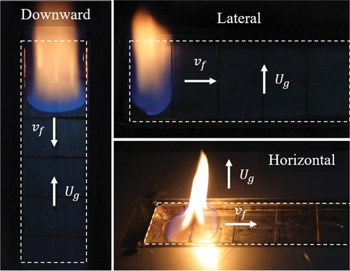
There are, however, multiple sample configurations that can exhibit opposed-flow flame spread, as illustrated in Figure 1; each configuration displays a characteristically different flame shape, and thus differing relative contributions from each heat transfer mechanism. Opposed-flow flame spread can, therefore, be further subdivided into additional regimes to better describe flame spread behavior. The magnitude of each heat transfer mechanism was quantified using a methodology developed by Ito and Kashiwagi (Ito and Kashiwagi 1988). This study builds on this original work, comparing the configurations seen in Figure 1 and allows for the analysis to be conducted using relatively simple thermocouple measurements in the solid phase.

Figure 1. Regimes of opposed flow spread: downward, horizontal, and lateral spread.

Background

The process of flame spread is described as an advancing ignition front over a solid where the flame front acts as both the heat source to initiate pyrolysis and the pilot to ignite the flammable pyrolysis gases (Drysdale 2011; Quintiere 2006). The rate of spread is then controlled by the heat transfer mechanisms from the flame (Fernandez-Pello and Hirano 1983). Comprehensive reviews of opposed flow flame spread are provided by Wichman (Wichman 1992), Fernandez-Pello & Hirano (Fernandez-Pello and Hirano 1983), and Hasemi (Hasemi 2016). Additional references on the fundamentals of flame spread include Drysdale (Drysdale 2011), Quintiere (Quintiere 2006), and Fernandez-Pello (Fernandez-Pello 1995).

Opposed flow spread has traditionally been conceptualized as illustrated in Figure 2. The relevant heat transfer mechanisms are dependent on the interaction between the flame and the fuel surface.

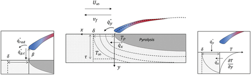
Figure 2. Middle: A schematic representation of the relevant heat transfer mechanisms dictating opposed flow flame spread. Left: A representation of the relevant gas phase heat transfer (both gas phase conduction and radiation). Right: a representation of conduction through the solid phase ahead of the flame front.

Heat transfer to the pyrolyzing material ahead of the flame front occurs due to three key mechanisms: solid-phase conduction, gas-phase conduction, and radiation from the flame. The degree to which any one of these mechanisms contributes to the flame spread rate depends on both the conditions surrounding the sample and the geometric properties of the material. Previous studies, for example, have shown that the relative contribution of the gas-phase conduction contributes a larger proportion of the total heat transfer for thin materials compared to thicker materials. The classification of thin and thick materials is system dependent, but previous studies on flame spread have coarsely defined thin being less than 2 mm and thick being more than 20 mm (Fernandez-Pello and Hirano 1983). The relative contribution of the solid-phase conduction term follows the opposite trend, showing less of a total contribution for thin solids and a larger contribution for thicker solids.

The aim of this study is to quantify the magnitude of these heat transfer processes and compare them across the different regimes of opposed flow spread identified in Figure 1. Figure 2 illustrates a flame anchored to the surface of a material where the freestream velocity, $U_{\mathrm{\infty }}$, moves in the opposite direction of flame spread, $v_f$. The region beneath the flame is pyrolyzing; the depth of the pyrolysis region decreases closer to the flame front. The flame front is defined at x = 0; the following formulation effectively assumes the pyrolysis front and flame front exist at the same location, while in reality the pyrolysis front is likely to be present ahead of the leading edge of the flame due to upstream heat transfer. At x = 0 the surface pyrolysis occurs. Ahead of the flame front, temperatures at the surface gradually decrease; the length $\delta$ indicates the distance at which the surface is nearly ambient. Likewise, $\tau$ represents the depth at x = 0 at which the solid is approximately ambient. Following from this, the heat transfer ahead of the flame front can be defined over two control surfaces: the surface from x = 0 to x=$\delta$ over which gas-phase heat transfer occurs (Control Surface $\delta$); and the surface immediately below the flame front from y = 0 to y=$\tau$, over which heat is conducted ahead of the flame front through the solid (Control Surface $\tau$). This formulation closely resembles the methodology originally outline by Ito and Kashiwagi (Ito and Kashiwagi 1988).

Heat transfer conducted across Control Surface $\tau$ is driven by both already pyrolyzing material at the surface and heated material in-depth. The thermal gradients in-depth results in a distribution of conductive heat transfer, being highest near the surface and decreasing in-depth. The distribution of conductive heat fluxes across Control Surface $\tau$, ${\dot{q}}_x^{\prime \prime }$, is determined using Equation 1(1) ${{\dot{q}}_x}^{\prime \prime }=k_s{\left.\frac{\mathrm{\partial }{T}_s}{\mathrm{\partial }x}\right|}_{x=0}$(1) and the integrated conductive heat transfer over Control Surface $\tau$, $Q_c$, is determined using Equation 2(2) ${\dot{Q}}_x^{\prime }\hspace{0.17em}={\int }_{\tau }^0{k}_s{\left.\frac{\mathrm{\partial }{T}_s}{\mathrm{\partial }x}\right|}_{x=0}dy$(2) (Ito and Kashiwagi 1988).

(1) ${{\dot{q}}_x}^{\prime \prime }=k_s{\left.\frac{\mathrm{\partial }{T}_s}{\mathrm{\partial }x}\right|}_{x=0}$(1)

(2) ${\dot{Q}}_x^{\prime }\hspace{0.17em}={\int }_{\tau }^0{k}_s{\left.\frac{\mathrm{\partial }{T}_s}{\mathrm{\partial }x}\right|}_{x=0}dy$(2)

Heat transfer from the flame to the solid occurs through both gas-phase conduction, ${\dot{q}}_{g,c}^{{ }^{\prime \prime }}$, and radiation, ${\dot{q}}_{rad}^{{ }^{\prime \prime }}$. Both these terms are represented as gradients – being highest at the flame front and decreasing toward x=$\delta$ (Ito and Kashiwagi 1988). The total heat transfer across Control Surface $\delta$ includes both gas-phase conduction and radiation (${\dot{q}}_y^{{ }^{\prime \prime }}={\dot{q}}_{g,c}^{{ }^{\prime \prime }}+{\dot{q}}_{rad}^{{ }^{\prime \prime }}$) but also includes heat losses from the surface (${\dot{q}}_{l,surf}^{\prime \prime }$); surface losses are assumed to be limited to radiative losses throughout this study (an emissivity of 0.9 assumed throughout (Girods et al. 2011)). Gas phase conduction transfers heat from the flame to the surface over the standoff distance, $\beta$ as seen in Figure 2. Equation 3(3) ${{\dot{q}}_y}^{\prime \prime }={{\dot{q}}_{g,c}}^{\prime \prime }+{{\dot{q}}_{rad}}^{\prime \prime }=k_s{\left.\frac{\mathrm{\partial }{T}_s}{\mathrm{\partial }y}\right|}_{y=0}+{\dot{q}}_{l,surf}^{\prime \prime }$(3) can be used in combination with Equation 4(4) ${{\dot{q}}_{l,surf}}^{\prime \prime }=\epsilon \sigma \left(T_{surf}^4-T_{\mathrm{\infty }}^4\right)$(4) to express the heat flux gradient at the surface, and Equation 5(5) ${\dot{Q}}_y^{\prime }\hspace{0.17em}={\int }_0^{\delta }{{\dot{q}}_y}^{\prime \prime }dx$(5) can be used to approximate the integrated heat transfer to the surface.

(3) ${{\dot{q}}_y}^{\prime \prime }={{\dot{q}}_{g,c}}^{\prime \prime }+{{\dot{q}}_{rad}}^{\prime \prime }=k_s{\left.\frac{\mathrm{\partial }{T}_s}{\mathrm{\partial }y}\right|}_{y=0}+{\dot{q}}_{l,surf}^{\prime \prime }$(3)

(4) ${{\dot{q}}_{l,surf}}^{\prime \prime }=\epsilon \sigma \left(T_{surf}^4-T_{\mathrm{\infty }}^4\right)$(4)

(5) ${\dot{Q}}_y^{\prime }\hspace{0.17em}={\int }_0^{\delta }{{\dot{q}}_y}^{\prime \prime }dx$(5)

Experimental methods

This study presents results from bench-scale flame spread experiments using clear cast polymethyl methacrylate (PMMA) to observe downwards, lateral, and horizontal spread in the absence of a forced flow. Experiments were conducted using 50 × 200 × 12 mm samples. Flame spread rates were determined from video analysis and surface temperature measurements.

In-depth temperature measurements were taken using 0.75 mm diameter sheathed K-type thermocouples. Holes for each thermocouple location were drilled using a CNC mill. To ensure good contact at the thermocouple tip, each hole was countersunk, as per previous studies (Santamaria Garcia 2021). Temperature measurements were made at the surface by fusing 0.25 mm K-type thermocouples to the surface of the polymer sample. Temperatures were measured at six locations along the sample; further detail on instrument location and arrangement can be found in Appendix A. Video analysis was used to determine the progression of the flame front as a function of time. A MATLAB algorithm was used to identify the RGB intensity of each frame and isolate the blue pixel intensity; this allowed the progression of the blue flame front to be tracked, as per a previous study (Morrisset et al. 2022).

Polymer samples were placed in a machined aluminum sample holder that was bored with four 12 mm holes to allow for water cooling of the sample holder. Water temperatures were recorded at the inlet and outlet of the sample holder to determine the temperature of the sample back face and to indicate any change in water temperature while passing through the sample holder. Water cooling prevented the influence of edge effects and mitigated any preheating of the polymer from the sample holder.

Results

Flame spread rates were calculated using both video analysis and temperature measurements. Once the time resolved flame front position was established from the video data, this was differentiated to determine the flame spread rate. Average flame spread rates were also determined using the measured temperature data. Average flame spread rates were determined as $s/t_d$ where $s$ is the spacing between each measurement location (30 mm) and $t_d$ is the duration between the adjacent thermocouples reaching 350°C (the arrival of the flame front). Due to the limited number of measurement locations, the temperature data were only able to yield average flame spread rates between each location, while the video analysis allowed for highly resolved temporal measurements.

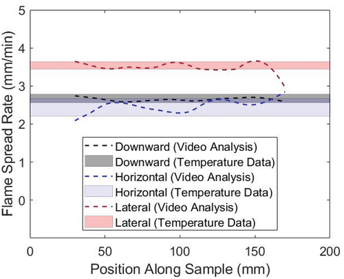
Calculated flame spread rates using both video analysis and temperature measurements are presented in Figure 3. Temporally resolved flame spread measurements from video analysis show good agreement within the range of average flame spread rates determined from temperature measurements. Average flame spread rates of 2.67 mm/min and 2.54 mm/min were recorded for downward and horizontal spread, respectively. Both downward and horizontal showed similar rates of spread; however, the observed downward spread rates were more consistent over the duration of each experiment, as indicated in the range of data presented in Figure 3. Lateral flame spread displayed the highest spread rate with an average of 3.54 mm/min with the same degree of consistency observed for downward spread. The degree of consistency for both downward and lateral spread is likely due to the strong vertical flame sheet established on the surface in comparison to the horizontal configuration where the buoyant plume above the sample flickers with time. Appendix B provides more information regarding the consistency of data recorded in the horizontal configuration.

Figure 3. Flame spread rates for each configuration determined using both video analysis and surface temperature measurements considering all measurement locations and repeat trials. Video data was averaged across repeat trials and was only analyzed between 30–170 mm.

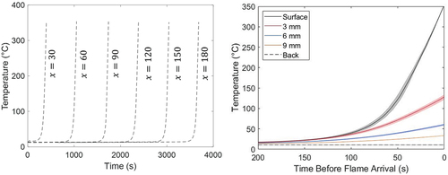
Figure 4 illustrates surface temperature measurements over the length of a tested sample. The uniform spacing between each surface thermocouple location indicating the arrival of the flame front (i.e., temperatures between 300°C and 350°C) illustrate steady state flame spread behavior. Figure 4 also shows temperature measurements in-depth as the flame approaches each station over the length of the sample – these data highlight the small degree of variation in thermal gradient at the flame front for each of the locations measured. Compared across each measurement location, the temperature time histories show a maximum variation of approximately 15% which is within the degree of repeatability observed between repeat experiments (Morrisset et al. 2021a, 2021b). The shaded region in Figure 4, therefore, indicates the consistency of the thermal gradient ahead of the flame front for each location along the sample which is further evidence of steady flame spread behavior.

Figure 4. The time histories of temperature measurements at each measurement location along the sample as the flame front approached. The consistent time histories observed as the flame front approaches each location indicates steady flame spread behavior. Data presented for downward flame spread. All x positions are presented in mm.

Analysis

Additional analysis using thermal gradients in the solid provides further insight into the relevant mechanisms of flame spread. The fact that the observed flame spread processes were steady allows thermal gradients throughout the solid to be estimated using the time history of the recorded temperatures. That is, a single set of in-depth thermocouples experience the full temperature history of the approaching flame front. Thus, these highly resolved temporal data can (under steady state flame spread conditions) be used to create highly resolved spatial data for the thermal conditions ahead of the flame front. This is achieved by a retroactive temperature reconstruction based on the observed rate of flame spread. At any measurement location, the thermal gradient in-depth at the flame front (i.e., $dT/dy$ at $x=0$) is determined as the recorded temperatures in-depth at $t_p$ (i.e., the time at which the surface thermocouple reaches 350°C). The thermal gradient at any position along the sample (i.e., $x=r$) can then be determined using the recorded temperature data evaluated at $t_p-\mathrm{\Delta }t$, where:

(6) $\mathrm{\Delta }t=\frac{r}{v_f}$(6)

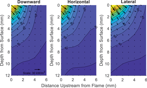
This process can be repeated for any spacing $r$ by using the steady state temperature history and flame spread rate to reconstruct the thermal gradient ahead of the flame front. The process of using Equation 6(6) $\mathrm{\Delta }t=\frac{r}{v_f}$(6) to reconstruct the temperature distribution can be seen in Figure 5 using a spacing of 1 mm. Complete reconstructions for each of the experimental configurations used in this study can be seen in Figure 6. These plots are notably similar to those created by Ito and Kashiwagi whose measurements were instead taken with holographic interferometry instead of in-depth thermocouples (Ito and Kashiwagi 1988). The reconstructed temperature fields are useful as they can highlight the differences in the approaching flame fronts for each configuration tested. While both the downward and horizontal spread show similar conditions along the surface ahead of the flame front (i.e., similar values of $\delta$), the lateral configuration displays a larger preheated distance ahead of the flame. These observations are discussed further in the analysis section of this work.

Figure 5. A graphical explanation of the temperature reconstruction method used in this study.

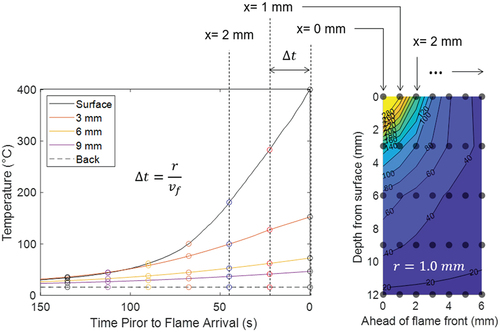
Figure 6. Simulated thermal distributions in the solid ahead of the flame front determined using the temperature reconstruction method. Distributions simulated for downward (left), horizontal (middle), and lateral (right) spread. All contours in °C.

Higher resolution thermal distributions ahead of the flame front not only lend general insight into the preheated areas ahead of the flame but also allow approximation of the relative contributions of each heat transfer mechanism as outlined in Equations 1(1) ${{\dot{q}}_x}^{\prime \prime }=k_s{\left.\frac{\mathrm{\partial }{T}_s}{\mathrm{\partial }x}\right|}_{x=0}$(1) -5(5) ${\dot{Q}}_y^{\prime }\hspace{0.17em}={\int }_0^{\delta }{{\dot{q}}_y}^{\prime \prime }dx$(5) . Figure 7 illustrates the thermal gradients both as a function of depth and distance from the flame front (i.e., $\frac{d{T}_s}{dx}$ and $\frac{d{T}_s}{dy}$). These gradients can be evaluated at the surface or along Control Surface $\tau$ and used in combination with the thermal conductivity of the solid to determine the rate of gas-phase heat transfer and solid-phase conduction (e.g., Equation 3(3) ${{\dot{q}}_y}^{\prime \prime }={{\dot{q}}_{g,c}}^{\prime \prime }+{{\dot{q}}_{rad}}^{\prime \prime }=k_s{\left.\frac{\mathrm{\partial }{T}_s}{\mathrm{\partial }y}\right|}_{y=0}+{\dot{q}}_{l,surf}^{\prime \prime }$(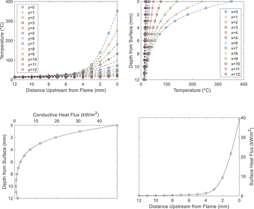3) which uses the gradients with respect to y to determine gas-phase conduction). Each heat flux contribution was calculated assuming a thermal conductivity of 0.27 W/m-K (Hurley et al. 2015). All positions between thermocouple measurements in depth (i.e., values in the y-direction between 0, 3, 6, 9 and 12 mm) were approximated using an exponential curve fit as seen in Figure 7.

Figure 7. Top figures: the thermal gradients ahead of the flame front in both the x and y direction. These gradients are then evaluated at either x=0 or y=0 for each depth or position along the surface, through which the conductive (${\dot{q}}_x^{{ }^{\prime \prime }}$) and gas phase (${\dot{q}}_y^{{ }^{\prime \prime }}$) heat transfer rates can be calculated (lower figures).

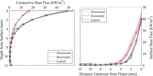
Figure 8 then compares the calculated heat flux distributions across the three configurations used in this study. The downward and horizontal configurations display similar heat flux distributions for both ${\dot{q}}_x^{{ }^{\prime \prime }}$ and ${\dot{q}}_y^{{ }^{\prime \prime }}$; the lateral configuration, however, displays a higher rate of heat transfer along the surface while displaying a lower rate of conductive heat transfer within the solid as determined using this method. These results suggest that the lateral configuration presents higher gas-phase heat transfer (i.e., a higher total heat flux from gas-phase conduction and radiation) compared to the other orientations; the increase in total heat flux is likely due to, in part, the increased radiation from the luminous portion of the leading edge (as seen in Figure 1).

Figure 8. A comparison of the conductive heat flux distribution (${\dot{q}}_x^{{ }^{\prime \prime }}$) and the gas phase heat flux distributions (${\dot{q}}_y^{{ }^{\prime \prime }}$) across the three configurations used in this study.

The distributions of ${\dot{q}}_x^{{ }^{\prime \prime }}$ and ${\dot{q}}_y^{{ }^{\prime \prime }}$ can then be used to determine the characteristic length scales of $\delta$ and $\tau$. Both $\delta$ and $\tau$ were defined as the location on each respective control surface exposed to a heat flux 5% of the value measured at the flame front. Table 1 compares the calculated results across each configuration tested, including flame spread rates, total integrated heat flux contributions, and the calculated characteristic length scales.

Table 1. Resulting flame spread rates, heat flux contributions, and relevant characteristic length scales as defined by Equations 1(1) ${{\dot{q}}_x}^{\prime \prime }=k_s{\left.\frac{\mathrm{\partial }{T}_s}{\mathrm{\partial }x}\right|}_{x=0}$(1) –4(4) ${{\dot{q}}_{l,surf}}^{\prime \prime }=\epsilon \sigma \left(T_{surf}^4-T_{\mathrm{\infty }}^4\right)$(4) .

Configuration	${\mathit{v}}_{\mathit{f}}$ (mm/min)	$\dot{{\mathbf{Q}}^{\prime }}x$ (W/m)	${\dot{\mathit{Q}}}_y^{\prime }$ (W/m)	${\dot{q}}_{f}2\delta$δ (kW^2/m)	Max ${{\dot{q}}^{″}}_y$ (kW/m^2)	Max ${\dot{\mathit{q}}}_{\mathit{x}}^{{ }^{\prime \prime }}$ (kW/m^2)	δ (mm)	τ (mm)
Downward	2.67 $\pm$ 0.13	106	57	1.23	41.2	50.6	3.6	6.4
Horizontal	2.54 $\pm$ 0.50	101	58	1.08	40.4	54.7	3.4	5.3
Lateral	3.54 $\pm$ 0.17	45	82	1.91	46.1	18.9	5.0	6.5

The results displayed in Table 1 indicate that the downward and horizontal configurations display similar flame spread rates, and also display similar contributions from both gas-phase heat transfer and conduction through the solid. While the values of $\delta$ agree between these two configurations, $\tau$ was observed to be approximately 20% shallower for the horizontal configuration as indicated by the temperature reconstruction seen in Figure 6. The lateral configuration displays both a higher flame spread rate and higher total integrated heat transfer to the surface, ${\dot{Q}}_y^{\prime }$. The higher value of ${\dot{Q}}_x^{\prime }$ is a result of higher values of ${\dot{q}}_y^{{ }^{\prime \prime }}$ along the surface and a larger preheated distance. Table 1 suggests that an increase in flame spread rate is related to an increasing value of ${\dot{Q}}_x^{\prime }$ and a decreasing value of ${\dot{Q}}_y^{\prime }$ (as determined with this method). This same trend was observed in the results presented by Ito and Kashiwagi (Ito and Kashiwagi 1988).

Various simple models for flame spread over thick solids suggest that $v_f\propto {{\dot{q}}^{″}}_{f}2\delta$, where ${\dot{q}}_f^{{ }^{\prime \prime }}$ is the assumed heat flux to the surface from the flame (Drysdale 2011; Quintiere 2006). This proportionality can be observed when comparing the across the configurations used in this study. The integrated value of ${{\dot{q}}^{″}}_{f}2\delta$ (i.e., $\underset{0}{\overset{\delta }{\int }}{\dot{q}}_y^{{ }^{\prime \prime }}dx$) is also presented in Table 1, which indicates a nearly linear relationship between an increase in ${{\dot{q}}^{″}}_{f}2\delta$ and the subsequent increase in flame spread rate. Therefore the proportionality suggested in existing flame spread models is observed here. The rate of increase in flame spread rate appears to be linked closest to the total heat flux received at the surface (i.e., a combination of ${\dot{q}}_y^{{ }^{\prime \prime }}$ and $\delta$).

Conclusions

This study presents an experimental investigation into three distinct configurations of opposed flow flame spread, to identify the relevant heat transfer mechanisms in each condition. Flame spread rates were determined using both video analysis and surface temperature measurements and were found to be of 2.67, 2.54, and 3.54 mm/min for downward, horizontal, and lateral spread, respectively. The thermal gradients ahead of the flame front were determined using a temperature reconstruction from in-depth temperature measurements. This approach allowed for the quantification of the relative heat flux contributions at the sample surface (i.e., gas-phase heat transfer to the surface from the flame) as well as conductive heat transfer from underneath the flame sheet to virgin material (i.e., conduction across Control Surface $\tau$).

The downward and horizontal configurations displayed a higher value of ${\dot{Q}}_x^{\prime }$ than ${\dot{Q}}_y^{\prime }$ which corresponds to claims from previous studies that conduction through the solid plays a larger role for opposed flow flame spread in thermally thick solids. The lateral configuration, however, displayed a higher contribution from gas-phase heat transfer than from conduction through the solid. These results suggest that the notably higher flame spread rate for the lateral configuration results, in part, from the enhanced gas-phase heat transfer in the lateral configuration and the higher temperatures observed along the surface ahead of the flame front.

This work builds on techniques employed in previous studies to demonstrate the relevant heat transfer mechanism for three unique opposed flow flame spread regimes and presents a methodology of temperature reconstruction to gain further insight into flame spread mechanics.

Disclosure statement

No potential conflict of interest was reported by the author(s).

Correction Statement

This article has been corrected with minor changes. These changes do not impact the academic content of the article.

Appendices Appendix A:

Location of thermocouple measurements and details on sample holder

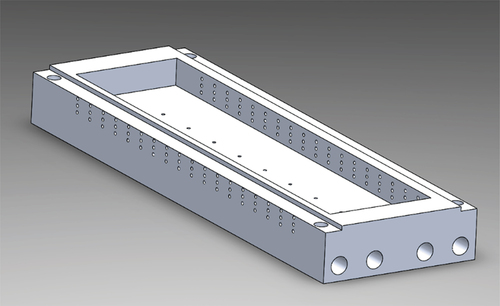
Figure A1 illustrates the distribution of temperature measurements throughout each sample tested. Each location indicates three in-depth 0.75 mm K-type thermocouples and as well as a 0.25 mm K-type thermocouple fused to the surface. The back face temperatures are determined by measuring the water temperature passing through the water cooled sample holder. For each experiment, the measured temperature rise in the water flowing through the sample holder was undetectable (i.e., less than the resolution of the thermocouples used). Figure A2 shows the aluminium sample holder used in this study.

Figure A1. A schematic representation of the thermocouple placement within each sample tested. At each location, three in-depth measurements were made in addition to a surface temperature measurement. Back face temperatures were measured from the temperatures recorded for the water cooling system. All dimensions in mm.

Figure A2. The water-cooled sample holder used in this study. Continuous water cooling was provided through the four holes passing through the length of the sample holder. Additional holes were milled through the sides of the sample holder to insert the thermocouples in-depth within the solid.

Appendix B:

Horizontal spread temperature distributions

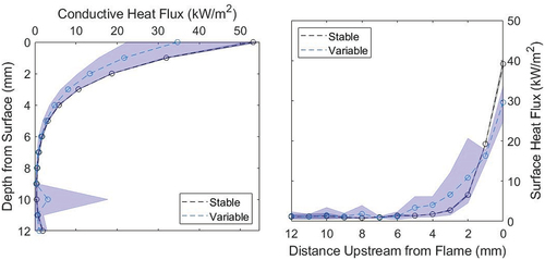
Stable temperature measurements are required for the temperature reconstruction method outlined in this work. Both downward and lateral flame spread displayed relatively stable temperature measurements in time across each measurement location (as previously seen in Figure 4). The horizontal configuration, however, displayed much less stable temperature measurements as seen in Figure B1.

Due to an inability to control the variability seen for the turbulent stations, only the stable readings from each experiment were processed and compared throughout the analysis of this work. However the full data are presented here for clarity. In addition to high fluctuations at the surface, the variable stations displayed different trends for temperatures in depth as well. Stable measurements were achieved consistently for both downward and lateral spread. Figure B2 illustrates the variation observed in the calculated heat flux contributions between the stable and variable measurement locations.

Figure B1. Temperature time histories as the flame approaches each station for a horizontal flame spread trial. The first two stations display stable temperature readings (solid lines), while the remaining stations display a different heating behavior (dashed lines).

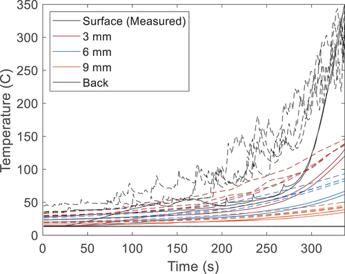
Figure B2. A comparison on the gas phase and conductive heat fluxes calculated for the stable temperature readings seen in Figure and the variable readings seen as the flame grows more turbulent.

References

- De Ris, J. N. 1968. The spread of a diffusion flame over a combustible solid. Diss. Harvard University.
- De Ris, J. N. 1969. Spread of a laminar diffusion flame Symposium (International) on Combustion 12 (1):241–52. doi:10.1016/S0082-0784(69)80407-8.
- Drysdale, D. 2011. An introduction to fire dynamics. 3rd ed. 10.1002/9781119975465.
- Fernandez-Pello, C. 1995. The Solid Phase. In Combustion Fundamentals of Fire, 31–100. Academic Press.
- Fernandez-Pello, A. C., and T. Hirano. 1983. Controlling mechanisms of flame spread. Combust. Sci. Technol 32 (1–4):1–31. doi:10.1080/00102208308923650.
- Fernandez-Pello, A., and F. A. Williams. 1975. Laminar flame spread over PMMA surfaces. Symposium (International) on Combustion 15 (1):217–31. doi:10.1016/S0082-0784(75)80299-2.
- Girods, P., H. Bal, H. Biteau, G. Rein, and J. Torero. 2011. Comparison of pyrolysis behavior results between the cone calorimeter and the fire propagation apparatus heat sources. Fire Saf. Sci. 10:889–901. doi:10.3801/IAFSS.FSS.10-889.
- Hasemi, Y. 2016. Surface flame spread. In SFPE handbook of fire protection Engineering 705–23. Springer New York. doi:10.1007/978-1-4939-2565-0_23.
- M. J. Hurley, D. Gottuk, J. R. Hall, K. Harada, E. Kuligowski, M. Puchovsky, J. Torero, J. M. Watts, and C. Wieczorek. 2015. SFPE handbook of fire protection engineering. Springer. doi:10.1007/978-1-4939-2565-0.
- Ito, A., and T. Kashiwagi. 1988. Characterization of flame spread over PMMA using holographic interferometry sample orientation effects. Combust. Flame 71 (2):189–204. doi:10.1016/0010-2180(88)90007-7.
- Morrisset, D., Hadden, R., Law, A., and Torero, J. 2022. Downward flame spread over PMMA spheres. Proc. Combust. Inst 39 (3):4155–4164. doi:10.1016/j.proci.2022.07.220.
- Morrisset, D., Thorncroft, G., Hadden, R., Law, A., and Emberley, R. 2021a. Sequential analysis for quantifying statistical uncertainty in fire testing. 12th Asia-Oceania Symposium on Fire Science and Technology, Brisbane, Australia.
- Morrisset, D., Thorncroft, G., Hadden, R., Law, A., and Emberley, R. 2021b. Statistical uncertainty in bench-scale flammability tests. Fire safety journal 122:103335. doi:10.1016/j.firesaf.2021.103335.
- Quintiere, J. 2006. Fundamentals of fire phenomena. Wiley.
- Santamaria Garcia, S. 2021. Ignition of solids exposed to transient irradiation. PhD diss., The University of Edinburgh.
- Wichman, I. S. 1992. Theory of opposed-flow flame spread. Prog. Energy Combust. Sci. 18 (6):553–93. Elsevier. doi:10.1016/0360-1285(92)90039-4.