A Numerical Study of Flow Structures and Flame Shape Transition in Swirl-Stabilized Turbulent Premixed Flames Subject to Local Extinction

ABSTRACT

Large Eddy Simulations (LES) of turbulent lean-premixed flames of V- and M-shape are presented. A simple algebraic closure with the ability to capture finite-rate chemistry effects is used for subgrid reaction rate modeling. The V-shaped flame is stabilized in the inner shear layer between a swirling annular jet and a central recirculating bubble in a sudden expansion duct. The M-shaped flame is stabilized in the inner and outer shear layer, adjoining the corner recirculation zone induced by the vertical step. The focus of the study is on the flow fields and shapes of the flames, which distinguish themselves through different heat load and sensitivity to local extinction. Good agreement with measurements is observed for the cold and the reacting flow cases. The numerical results suggest that the entrainment of hot gases into the outer recirculation zone occurs close to the impingement point of the swirling annular jet on the wall and this process is strongly dependent on intense vortical structures in the outer shear layer. The results further suggest that local extinction influences the position of the flame in the inner shear layer and, thereby, also the intensity of the local entrainment process.

KEYWORDS:

• Lean premixed combustion
• LES
• progress variable reaction rate
• dissipation
• OpenFOAM

Introduction

Lean premixed combustion has recently gained much attention in light of increasingly stringent environmental standards. Large Eddy Simulation (LES) has been applied successfully to turbulent premixed combustion problems of considerable complexity, e.g. (Galpin et al. 2008; Guo et al. 2019; Wang et al. 2013) as was also reviewed by Steinberg, Hamlington, and Zhao (2021). Lean premixed combustion can be characterized by comparatively large chemical time scales and moderate heat release rates. Wang et al. (2013) stated that the increased chemical time scales observed in lean premixed flames can lead to extinction and reignition phenomena under the influence of turbulence. LES modeling studies of premixed flames undergoing local extinction are scarce in the literature. Chen et al. (2020) and Wang et al. (2013) studied partially premixed and premixed turbulent flames, respectively, using LES with presumed probability density function (PDF) approach. The former was connected to unstrained steady laminar flamelets, the latter to a reaction-diffusion manifold approach. An important aspect of the limited availability of numerical studies of flames showing (local) extinction phenomena is the constrained validity of many combustion models under these conditions. Meneveau and Poinsot (1991) stated that flame quenching by turbulence, where chemical kinetics in the reaction zones are quenched by high stretch, is an important process influencing the validity of the commonly applied flamelet assumption, describing the reaction zone as an almost infinitely thin interface between burnt and unburnt material (Peters 1988). In addition, underlying mechanisms of (local) extinction in premixed flames are highly complex, and the role of scalar dissipation in them is not yet fully understood, as stated by Chen et al. (2020). A number of studies have indicated a linkage with Damköhler number. Shanbhogue, Husain, and Lieuwen (2009), for example, analyzed a large data set on extinction in premixed bluff body flames available in the literature and found correlations with different formulations of the Damköhler number. Dunn, Masri, and Bilger (2007) studied strong finite-rate chemistry effects in a turbulent premixed piloted flame and explained the observed onset of local extinction as a phenomenon of high dissipation rates and a reduction of Damköhler number. Stöhr, Arndt, and Meier (2013) studied three premixed flames with varying Damköhler numbers and observed local disruptions and downstream shifting of the reaction zones for low Damköhler numbers, which were related to vortex-induced stretch.

Shanbhogue et al. (2016) investigated swirl-stabilized flames with different heat load in a dump combustor and related the observed flame shape transitions to local extinction in the highly strained shear layers. For increasing thermal power, keeping the same flow conditions, they noted that the flame extended from the inner shear layer to the corner recirculation zone and, eventually, also stabilized in the outer shear layer. This behavior was also observed for other modifications of operating conditionsfor example, by varying the Lewis number (Guiberti et al. 2015) or thermal boundary conditions (Guiberti et al. 2015; Mercier et al. 2016). The transition between these two common flame shapes, often referred to as V- and M-shaped flames, has kindled much research interest. This has been connected to the general striving for a better understanding of premixed flames relevant for gas turbine combustion (Langella et al. 2019; Taamallah et al. 2015), but also to recent findings that indicated beneficial behavior of M-shaped flames for example, the higher operation stability described by Krikunova (2019). The mechanisms leading to the transitions are not well understood (Guiberti et al. 2015) and the different causes of flashback (Fritz, Kröner, and Sattelmayer 2004) in lean premixed combustion suggest a strong configuration dependence.

Many studies have investigated the influence of heat release on the development of the flow field in lean premixed turbulent flames. Robin, Mura, and Champion (2011) stated that the impact of thermal expansion on flow structures, both large- and small-scale, can be stronger than the influence of turbulence. Sabelnikov and Lipatnikov (2017) described the different pathways for flame–turbulence interaction in turbulent premixed combustion. The combustion-induced heat release is known to introduce both flame-generated turbulence and pressure perturbation. In the opposite direction, flow non-uniformities and turbulence influence the flame through local flow conditions and the flame surface. From many past studies on the influence of heat release, it becomes clear that the treatment of complex chemistry is secondary to understanding the development of the reacting flow field in lean turbulent premixed flames. This has also been noted by Lipatnikov et al. (2018). A key requirement of combustion models for this type of flame lies in the accurate prediction of local heat release and its effect on quantities, such as density, pressure and velocity. This allows the use of algebraic combustion models with a basic description of chemistry effects as long as the heat release can be captured accurately.

The aim of this study is to use a recently introduced algebraic filtered reaction rate formulation for the progress variable (Tomasch et al. 2022) to model premixed swirl-stabilized turbulent flames of two different lean equivalence ratios, where at least one undergoes local extinction. As the inflow conditions are kept constant for both flames, a change in the equivalence ratio corresponds to altering the heat load within the burner. The two investigated flames are of V- and M-shape, respectively, and this study aims to predict their behavior focusing on thermal effects and considering extinction phenomena through local chemical to flow time-scale ratios, omitting complex chemistry. The simulated burner was investigated experimentally in a number of studies (Kewlani, Shanbhogue, and Ghoniem 2016; Shanbhogue et al. 2016; Watanabe et al. 2016), also in LES using the Thickened Flame model (Kewlani, Shanbhogue, and Ghoniem 2016; Taamallah et al. 2019). Extensive flow data are available for cross-comparison of cold flow and V- and M-shaped flames. Mean and rms velocity data are first used to validate the simulation results, followed by an analysis of the reacting flow fields. In this study, the algebraic filtered reaction rate model from Tomasch et al. (2022) is extended to include contributions to turbulent reactions from the resolved scales. This modification becomes relevant when the local flame structures are partially resolved by LES.

Case description

The confined burner considered in this study is described in detail by Shanbhogue et al. (2016); Watanabe et al. (2016) and also in past numerical studies (Kewlani, Shanbhogue, and Ghoniem 2016; Taamallah et al. 2019). This burner is shown in Figure 1 and it consists of two concentrical ducts connected through a sudden expansion with an expansion ratio of 2. The upstream inlet duct has a diameter of $D=0.038\mathrm{m}$ and, for experiments, included a swirler at $L_{\mathrm{i}\mathrm{n}}\approx 1.5D$ upstream of the expansion plane. The axial swirler applied in the experiments has eight wedge-shaped vanes with a ${45}^{\circ }$ vane angle and a centerbody with a blockage ratio of approximately $24\mathrm{\%}$. The streamlined centerbody with tapered front and back tail has a base diameter of $9\mathrm{m}\mathrm{m}$ and a cone angle of ${60}^{\circ }$ (Taamallah et al. 2014). Experimental studies report a swirl number $S=0.7$ based on the vane angle $\alpha$. The Reynolds number based on the inlet diameter is $R{e}_{\mathrm{i}\mathrm{n}}\approx 20000$. No turbulence generator was employed in the experiments (Shanbhogue et al. 2016), and the turbulence field developed naturally from the wake of the swirler. The length of the burner section $L_{\mathrm{B}}$ is $0.4\mathrm{m}$, and the outlet is open to the atmosphere.

Figure 1. Schematic of the experimental burner (Kewlani, Shanbhogue, and Ghoniem 2016; Shanbhogue et al. 2016; Taamallah et al. 2019; Watanabe et al. 2016) with important features of the swirl-stabilized flow. IRZ denotes the inner recirculation zone, ORZ the outer, ISL and OSL are inner and outer shear layers, respectively. The yellow lines denote the position of the flame branches in the ISL for the V-shaped flame, the orange lines represent the flame boundaries in an M-shaped flame.

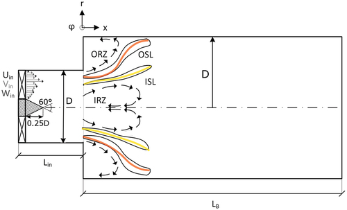
Next, the expected mean flow field will be described. For general notions on swirling combusting flows, the reader is referred to Lieuwen (2012), the case-specific behavior is thoroughly documented (Kewlani, Shanbhogue, and Ghoniem 2016; Shanbhogue et al. 2016; Taamallah et al. 2019; Watanabe et al. 2016), representative of numerous studies using this burner. An overview of the expected mean flow structures for the investigated case is given in Figure 1. The flow field (hot and cold) for this geometry and setup is controlled by a vortex bubble forming an inner recirculation zone (IRZ) at the centerline, and by an outer recirculation zone (ORZ) in the corner of the vertical step downstream of the expansion plane. The inner (center) and outer (corner) recirculation zones are marked schematically in Figure 1. In the expansion duct, shear layers form in regions between the incoming swirling annular jet and the recirculation zones. The inner shear layer (ISL) is located along the IRZ and the outer shear layer along the ORZ. Their interaction with the flame determines the flame shape (Taamallah et al. 2015). The V-shaped flame is located in the ISL only, indicated in Figure 1 by the two yellow lines representing the inner flame branches. The M-shaped flame is present in both the ISL and OSL, yellow and orange lines in Figure 1, and characterized by a coherent flame extending between the inner and outer shear layer.

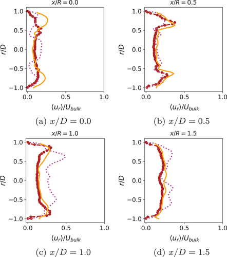
Different measurements are available from the experiments, among them detailed mean and rms velocity data for the axial, radial and tangential components of cold, and reacting flows at different equivalence ratios, and for five different locations downstream of the expansion plane ($x=0$) at $x/D=0$, 0.5, 1.0, 1.5 and 2.0 (Kewlani, Shanbhogue, and Ghoniem 2016; Taamallah et al. 2019). The flow features such as IRZ, ORZ, ISL, OSL are captured by the measured statistics since these features form around $1.5D$ downstream of the swirler at $x\approx 0$. The flow in the inlet duct is not measured and characterized.

LES modeling

Combustion closure

LES solves filtered transport equations, in case of premixed combustion, for momentum, enthalpy, mass, progress variable and progress variable variance. LES resolves the large-scale structures of the flow but requires closure to include the effects of the subgrid-scale (SGS) turbulence. Comprehensive descriptions of the theory behind LES are given elsewhere in the literature, for example, by Lesieur, Métais, and Comte (2005). In the subsequent discussion of transport equations, the over-bar and tilde denote LES- and Favre-filtering operations, respectively. The filtered momentum equation contains the unknown SGS stress tensor ${\tau }_{ij}=\widetilde{u_i{u}_j}-{\tilde{u}}_i{\tilde{u}}_j$, where $u_i$ is the velocity vector in the direction $i$. In this study, a $k$-equation model is used, which is based on the work from Yoshizawa (1986). The $k$-equation model involves solving a transport equation for the SGS kinetic energy $k_{\mathrm{s}\mathrm{g}\mathrm{s}}={\tau }_{kk}/2=\left(\widetilde{u_k{u}_k}-{\tilde{u}}_k{\tilde{u}}_k\right)/2$. The eddy viscosity is calculated using ${\mu }_{\mathrm{t}}=C_k\bar{\rho }\sqrt{k_{sgs}}\mathrm{\Delta }$, where $C_{\mu }=0.094$ is a model constant and $\mathrm{\Delta }$ the filter width based on the cube root of the local cell volumes. The filtered density is denoted by $\bar{\rho }$. The SGS scalar fluxes are modeled using the gradient approximation, and the SGS eddy diffusivity is expressed as ${\mu }_{\mathrm{t}}/S{c}_{\mathrm{t}}$ with the turbulent Schmidt or Prandtl number being $S{c}_{\mathrm{t}}=0.7$.

In this study, the combustion process is tracked using a progress variable defined by Bray, Champion, and Libby (2010), involving the mass fractions $Y_i$ of fuel (F) and oxygen,

(1) $c=\frac{(Y_{{\mathrm{O}}_2,\mathrm{u}}-Y_{{\mathrm{O}}_2,\mathrm{b}})(Y_{{\mathrm{O}}_2,\mathrm{u}}-Y_{{\mathrm{O}}_2})+(Y_{\mathrm{F},\mathrm{u}})(Y_{\mathrm{F},\mathrm{u}}-Y_{\mathrm{F}})}{{(Y_{{\mathrm{O}}_2,\mathrm{u}}-Y_{{\mathrm{O}}_2,\mathrm{b}})}^2+{(Y_{\mathrm{F},\mathrm{u}})}^2}.$(1)

This formulation ensures boundedness between the two states, unburnt (u; $c=0$) and fully burnt (b; $c=1$) mixture and unambiguously relates the quantity to a fully defined thermo-chemical state for a given fresh gas composition. The transport equation for the filtered progress variable is (Veynante and Vervisch 2002)

(2) $\overline{\rho }\frac{D\tilde{c}}{Dt}=\nabla \left[\left(\tilde{\mu }+\frac{{\mu }_{\text{t}}}{S{c}_{\text{t}}}\right)\nabla \tilde{c}\right]+{\overline{\dot{\omega }}}_c.$(2)

The filtered reaction rate ${\overline{\dot{\omega }}}_c$ is unknown and requires modeling. The closure of ${\overline{\dot{\omega }}}_c$ in this study is based on the model expression described by Tomasch et al. (2022), modified by including an additional term to consider reactions at resolved scales. For a detailed derivation of this closure model for ${\overline{\dot{\omega }}}_c$, the reader is referred to Tomasch et al. (2022).

As chemical reactions generally take place at small scales, ${\overline{\dot{\omega }}}_c$ is naturally interlinked with the behavior of $c$ at subgrid-scale level, which is treated statistically by solving a transport equation for the SGS progress variable variance defined as ${\sigma }_{c,\mathrm{s}\mathrm{g}\mathrm{s}}^2=\widetilde{c^2}-{\tilde{c}}^2$ (Veynante and Vervisch 2002). This transport equation is,

(3) $\overline{\rho }\frac{D{\sigma }_{c,\text{sgs}}^2}{Dt}=\nabla \left[\left(\tilde{\mu }+\frac{{\mu }_{\text{t}}}{S{c}_{\text{t}}}\right)\nabla {\sigma }^2{}_{c,\text{sgs}}\right]+2\frac{{\mu }_{\text{t}}}{S{c}_{\text{t}}}\left(\nabla \tilde{c}\nabla \tilde{c}\right)-2\overline{\rho }{\tilde{\chi }}_{c,\text{sgs}}+2\left[\overline{{\dot{\omega }}_{c}c}-{\overline{\dot{\omega }}}_c\tilde{c}\right].$(3)

The unknown terms in Eq 3(3) $\overline{\rho }\frac{D{\sigma }_{c,\text{sgs}}^2}{Dt}=\nabla \left[\left(\tilde{\mu }+\frac{{\mu }_{\text{t}}}{S{c}_{\text{t}}}\right)\nabla {\sigma }^2{}_{c,\text{sgs}}\right]+2\frac{{\mu }_{\text{t}}}{S{c}_{\text{t}}}\left(\nabla \tilde{c}\nabla \tilde{c}\right)-2\overline{\rho }{\tilde{\chi }}_{c,\text{sgs}}+2\left[\overline{{\dot{\omega }}_{c}c}-{\overline{\dot{\omega }}}_c\tilde{c}\right].$(3) are the SGS scalar dissipation rate ${\tilde{\chi }}_{c,\mathrm{s}\mathrm{g}\mathrm{s}}$ and a chemical reaction term ${\dot{\omega }}_{c}c\prime \prime =\left[\overline{{\dot{\omega }}_{c}c}-{\overline{\dot{\omega }}}_c\tilde{c}\right]$. They represent the processes of micro-mixing and chemical reaction that control the evolution of the SGS progress variable variance field and need to be modeled together with ${\overline{\dot{\omega }}}_c$ from Eq 2(2) $\overline{\rho }\frac{D\tilde{c}}{Dt}=\nabla \left[\left(\tilde{\mu }+\frac{{\mu }_{\text{t}}}{S{c}_{\text{t}}}\right)\nabla \tilde{c}\right]+{\overline{\dot{\omega }}}_c.$(2) . The micro-mixing is modeled using an algebraic closure (Dunstan et al. 2013) for the SGS scalar dissipation rate,

(4) ${\tilde{\chi }}_{c,\mathrm{s}\mathrm{g}\mathrm{s}}\simeq \left[1-exp\left(-0.75\mathrm{\Delta }/{\delta }_{\mathrm{t}\mathrm{h}}\right)\right]\left[\left(2K_c^{\ast }-\tau C_4\right)\frac{S_{\mathrm{L},0}}{{\delta }_{\mathrm{t}\mathrm{h}}}+C_3\frac{{\text{isin}}_{\mathrm{s}\mathrm{g}\mathrm{s}}}{k_{\mathrm{s}\mathrm{g}\mathrm{s}}}\right]\frac{{\sigma }_{c,\mathrm{s}\mathrm{g}\mathrm{s}}^2}{\beta { }^{\mathrm{\prime }}},$(4)

The relevant parameters appearing in the above model expression (Eq 4(4) ${\tilde{\chi }}_{c,\mathrm{s}\mathrm{g}\mathrm{s}}\simeq \left[1-exp\left(-0.75\mathrm{\Delta }/{\delta }_{\mathrm{t}\mathrm{h}}\right)\right]\left[\left(2K_c^{\ast }-\tau C_4\right)\frac{S_{\mathrm{L},0}}{{\delta }_{\mathrm{t}\mathrm{h}}}+C_3\frac{{\text{isin}}_{\mathrm{s}\mathrm{g}\mathrm{s}}}{k_{\mathrm{s}\mathrm{g}\mathrm{s}}}\right]\frac{{\sigma }_{c,\mathrm{s}\mathrm{g}\mathrm{s}}^2}{\beta { }^{\mathrm{\prime }}},$(4) ) are provided along with their values in Table 1 for the two flames investigated here. They are denoted as Flame III and Flame IV according to their naming in experiments (Kewlani, Shanbhogue, and Ghoniem 2016; Shanbhogue et al. 2016; Taamallah et al. 2019; Watanabe et al. 2016). Among other sources, Gao, Chakraborty, and Swaminathan (2014) provides a description of the individual parameters and their meaning. Where available, their relation to the fundamental laminar flame problem is given in Table 1. Calculations of these parameters are based on the solution of unstrained laminar premixed flames in Cantera (Goodwin et al. 2015) with the GRI-Mech 3.0 (Smith et al., nd) chemical mechanism. For this parameter ${\beta }^{\prime }$ a suitable value has to be set. There is some uncertainty inherent to the choice of this parameter in LES as has been described, for example, by Gao, Chakraborty, and Swaminathan (2014). This is due to its dependence on the turbulence modeling approach (LES) and combustion problem-related aspects such as heat release and turbulence Reynolds number. Despite this, ${\beta }^{\prime }$ has a strong influence on the scalar dissipation rate, changing with $\frac{\tilde{c}(1-\tilde{c})}{{\beta }^{\prime }}$. In this study, the parameter ${\beta }^{\prime }$ is of similar order of magnitude as the one used by Tomasch et al. (2022), and the one determined by Dunstan et al. (2013) carrying out a priori analysis of DNS data from a turbulent V-shaped flame. Gao, Chakraborty, and Swaminathan (2014) proposed a dependence of ${\beta }^{\prime }$ on the global heat release parameter $\tau$ described in Table 1, which results in slightly different values for ${\beta }^{\prime }$ in the two investigated flames. To better understand its impact on the simulations results, additional simulations are carried out varying this parameter. In the LES formulation of the algebraic closure of scalar dissipation rate proposed by Dunstan et al. (2013), a factor $\mathcal{F}=\left[1-exp\left(-0.75\mathrm{\Delta }/{\delta }_{\mathrm{t}\mathrm{h}}\right)\right]$ is used to ensure that the SGS scalar dissipation rate diminishes for $\mathrm{\Delta }/{\delta }_{\mathrm{t}\mathrm{h}}\to 0$.

Table 1. Various parameters of Eq 4(4) ${\tilde{\chi }}_{c,\mathrm{s}\mathrm{g}\mathrm{s}}\simeq \left[1-exp\left(-0.75\mathrm{\Delta }/{\delta }_{\mathrm{t}\mathrm{h}}\right)\right]\left[\left(2K_c^{\ast }-\tau C_4\right)\frac{S_{\mathrm{L},0}}{{\delta }_{\mathrm{t}\mathrm{h}}}+C_3\frac{{\text{isin}}_{\mathrm{s}\mathrm{g}\mathrm{s}}}{k_{\mathrm{s}\mathrm{g}\mathrm{s}}}\right]\frac{{\sigma }_{c,\mathrm{s}\mathrm{g}\mathrm{s}}^2}{\beta { }^{\mathrm{\prime }}},$(4) for SGS scalar dissipation rate modeling. $T_{ad}$ is the the adiabatic flame temperature in Kelvin, $T_0=298\mathrm{K}$ is the initial temperature, $S_{\mathrm{L},0}$ is the laminar flame speed, ${\delta }_{\mathrm{t}\mathrm{h}}$ is the thermal flame thickness and $K{a}_{\mathrm{\Delta }}={\left(\sqrt{2k_{\mathrm{s}\mathrm{g}\mathrm{s}}/3}/S_{\mathrm{L},0}\right)}^{3/2}{\left({\delta }_{\mathrm{t}\mathrm{h}}/\mathrm{\Delta }\right)}^{1/2}$.

Parameter	${\beta }^{\prime }$	$K_c^{\ast }$	$\tau$	$C_4$	$C_3$	$S_{\mathrm{L},0}$	${\delta }_{\mathrm{t}\mathrm{h}}$
Related to	-	thermo-chemistry	global heat release	$K{a}_{\mathrm{\Delta }}$		laminar flamelet
Formula	-	$K_c^{\ast }=0.79\tau$	$\tau =\frac{(T_{\mathrm{a}\mathrm{d}}-T_0)}{T_0}$	$\frac{1.1}{{(1+K{a}_{\mathrm{\Delta }})}^{0.4}}$	$\frac{1.5\sqrt{K{a}_{\mathrm{\Delta }}}}{1+\sqrt{K{a}_{\mathrm{\Delta }}}}$	-	$\frac{(T_{\mathrm{a}\mathrm{d}}-T_0)}{\mathrm{\nabla }T{|}_{\mathrm{m}\mathrm{a}\mathrm{x}}}$
Dimensions	$[]$	$[]$	$[]$	$[]$	$[]$	$[m/s]$	$[m]$
Flame III	3.5	3.55	4.59	-	-	0.11	0.001
Flame IV	4.0	3.85	4.88	-	-	0.15	0.0008

The expression for $\overline{{\dot{\omega }}_{c}c}$ used in this study follows the arguments of Bray (1979), where a simple model was used for this quantity,

(5) $\left[\overline{{\dot{\omega }}_{c}c}-{\overline{\dot{\omega }}}_c\tilde{c}\right]\approx (c_m-\tilde{c})1pt{\overline{\dot{\omega }}}_c.$(5)

The model parameter $c_m$ commonly takes values in the range of 0.7 to 0.8. The expression is strictly valid for large local Damköhler numbers, but it is shown (Chakraborty and Swaminathan 2011; Nilsson et al. 2019) to hold quite well also for moderate to low local Damköhler numbers.

The SGS progress variable variance contains valuable information on the structure of the reacting zones. The limiting case is fast chemistry or mixing-controlled combustion, where ${\sigma }_{c,\mathrm{s}\mathrm{g}\mathrm{s}}^2$ is $\tilde{c}\left(1-\tilde{c}\right)$, describing a double delta PDF. The segregation factor is defined as,

(6) $g=\frac{{\sigma }_{c,\mathrm{s}\mathrm{g}\mathrm{s}}^2}{\tilde{c}(1-\tilde{c})},$(6)

and the mixing-controlled combustion corresponds to $g=1$. Under realistic combustion conditions, $g$ is often smaller than one. The difference between the maximum and transported variances, given by

(7) ${\sigma }_{c,\mathrm{d}\mathrm{i}\mathrm{f}\mathrm{f}}^2=\tilde{c}\left(1-\tilde{c}\right)-{\sigma }_{c,\mathrm{s}\mathrm{g}\mathrm{s}}^2=\tilde{c}\left(1-\tilde{c}\right)\left(1-g\right),$(7)

has been denoted as the mixing factor by Bray (2011). The filtered reaction rate is obtained using

(8) ${\overline{\dot{\omega }}}_c=\underset{\text{I}}{\underbrace{A1pt\tilde{D}\left(\nabla \tilde{c}\cdot \nabla \tilde{c}\right)}}+\underset{\text{II}}{\underbrace{\overline{\rho }ℱ\left[a^{*}\left(c_{+}^{*}-c\right)+\left(1-a^{*}\right)\left(c-c_{-}^{*}\right)\right]/{\tau }_{\text{f}}}},$(8)

which comes from an algebraic closure of the general form ${\bar{\dot{\omega }}}_c=\mathcal{A}\left[\tilde{D}\mathrm{\nabla }\tilde{c}\cdot \mathrm{\nabla }\tilde{c}+\mathcal{F}\bar{\rho }{\sigma }_{c,\mathrm{s}\mathrm{g}\mathrm{s}}^2/{\tau }_{\mathrm{f}}\right]$ (Gao, Chakraborty, and Swaminathan 2014), consisting of a resolved ($\mathrm{I}$) and unresolved part ($\mathrm{I}\mathrm{I}$). In term $\mathrm{I}$, $\tilde{D}$ is the diffusion coefficient and $\mathcal{A}$ is an intrinsic, non-adjustable model constant of the SGS reaction rate term that is a function of $\tilde{c}$ and $g$. It takes a maximum value of $A=2$ (Tomasch et al. 2022) for infinitely fast chemistry. The given SGS reaction rate term (II) is the same as the one used by Tomasch et al. (2022). The quantity ${\tau }_{\mathrm{f}}$ is the SGS turbulence timescale, ${\tau }_{\mathrm{f}}=k_{\mathrm{s}\mathrm{g}\mathrm{s}}/{\text{isin}}_{\mathrm{s}\mathrm{g}\mathrm{s}}$, and represents a mixing timescale with $k_{\mathrm{s}\mathrm{g}\mathrm{s}}$ and ${\text{isin}}_{\mathrm{s}\mathrm{g}\mathrm{s}}$ being the subgrid kinetic energy and its dissipation rate. The quantity $c^{\ast }$ is connected to the reacting state at the SGS-level and is conceptually related to the mixing factor through ${\sigma }_{c,\mathrm{d}\mathrm{i}\mathrm{f}\mathrm{f}}^2=c^{\ast }\left(1-c^{\ast }\right)$, forming the two roots of the quadratic equation

(9) $c_{-,+}^{\ast }=0.5\pm \sqrt{0.25-{\sigma }_{c,\mathrm{d}\mathrm{i}\mathrm{f}\mathrm{f}}^2}.$(9)

The deviation of the solution of Eq 9(9) $c_{-,+}^{\ast }=0.5\pm \sqrt{0.25-{\sigma }_{c,\mathrm{d}\mathrm{i}\mathrm{f}\mathrm{f}}^2}.$(9) from the limit case $c_{+,-}^{\ast }=0$ and $1$ for infinitely fast chemistry is connected to a mixing process without considerable reaction activity. The influence of this initial, rate-determining process strongly depends on the turbulence to chemical time-scale ratio in the considered flame (Pope and Anand 1985). The deviation from the fast chemistry limit also defines the weighting factor $a^{\ast }$ in Eq 8(8) ${\overline{\dot{\omega }}}_c=\underset{\text{I}}{\underbrace{A1pt\tilde{D}\left(\nabla \tilde{c}\cdot \nabla \tilde{c}\right)}}+\underset{\text{II}}{\underbrace{\overline{\rho }ℱ\left[a^{*}\left(c_{+}^{*}-c\right)+\left(1-a^{*}\right)\left(c-c_{-}^{*}\right)\right]/{\tau }_{\text{f}}}},$(8) , through a lever rule, as

(10) $a^{\ast }=\frac{\tilde{c}-c_{-}^{\ast }}{c_{+}^{\ast }-c_{-}^{\ast }}.$(10)

The difference between Eq 8(8) ${\overline{\dot{\omega }}}_c=\underset{\text{I}}{\underbrace{A1pt\tilde{D}\left(\nabla \tilde{c}\cdot \nabla \tilde{c}\right)}}+\underset{\text{II}}{\underbrace{\overline{\rho }ℱ\left[a^{*}\left(c_{+}^{*}-c\right)+\left(1-a^{*}\right)\left(c-c_{-}^{*}\right)\right]/{\tau }_{\text{f}}}},$(8) and the formulation used by Tomasch et al. (2022) is the influence of resolved scales on the reaction progress, denoted by Term I and the factor $\mathcal{F}$ (Dunstan et al. 2013) in Term II, which ensures that the SGS reaction rate contribution diminishes for $\mathrm{\Delta }/{\delta }_{\mathrm{t}\mathrm{h}}\to 0$. To close the combustion problem, the transport equation for sensible enthalpy $h$ is solved,

(11) $\overline{\rho }\frac{d\tilde{h}}{dt}=\nabla \cdot \left[\left(\tilde{\mu }+\frac{{\mu }_{\text{t}}}{P{r}_{\text{t}}}\right)\nabla \tilde{h}\right]+\overline{\dot{Q}}.$(11)

In this equation, the modeled heat release rate per unit volume, $\overline{\dot{Q}}={\overline{\dot{\omega }}}_c{Y}_{f,u}1pt\Delta h_{\text{LHV}}$ is based on the lower heating value (LHV) of the fuel, the unburnt fuel mass fraction in the mixture and the filtered reaction rate of the progress variable (Tomasch et al. 2022). The temperature calculation based on $h$ follows the approach used by Ruan, Swaminathan, and Darbyshire (2014). Thermophysical and transport properties, such as constant-pressure heat capacities and diffusion coefficients, are provided by the probability density function approach detailed in (Tomasch et al. 2022) as function of the filtered progress variable and its variance.

Equation 8(8) ${\overline{\dot{\omega }}}_c=\underset{\text{I}}{\underbrace{A1pt\tilde{D}\left(\nabla \tilde{c}\cdot \nabla \tilde{c}\right)}}+\underset{\text{II}}{\underbrace{\overline{\rho }ℱ\left[a^{*}\left(c_{+}^{*}-c\right)+\left(1-a^{*}\right)\left(c-c_{-}^{*}\right)\right]/{\tau }_{\text{f}}}},$(8) is capable of including SGS finite-rate chemistry effects through the deviation of the transported SGS progress variable variance from its maximum value $\tilde{c}(1-\tilde{c})$. For conditions where the local turbulence dissipation to chemical time-scale ratio falls considerably below unity i.e., ${\tau }_{\mathrm{f}}\ll {\tau }_{\mathrm{c}}$, with ${\tau }_{\mathrm{f}}=k_{\mathrm{s}\mathrm{g}\mathrm{s}}/{\text{isin}}_{\mathrm{s}\mathrm{g}\mathrm{s}}$ being defined in accordance with the algebraic reaction rate model. In the high-shear region, it is assumed that the interlink between the SGS dissipation and reaction rate applied to express Term II of Eq 8(8) ${\overline{\dot{\omega }}}_c=\underset{\text{I}}{\underbrace{A1pt\tilde{D}\left(\nabla \tilde{c}\cdot \nabla \tilde{c}\right)}}+\underset{\text{II}}{\underbrace{\overline{\rho }ℱ\left[a^{*}\left(c_{+}^{*}-c\right)+\left(1-a^{*}\right)\left(c-c_{-}^{*}\right)\right]/{\tau }_{\text{f}}}},$(8) does no longer hold. In experiments by Shanbhogue et al. (2016), a clear connection between local extinction and the flame shape was observed for the two combustion cases investigated, hence it is expected that the condition ${\tau }_{\mathrm{f}}\ll {\tau }_{\mathrm{c}}$ is relevant for this study. In this case, it is ensured that the SGS contribution to the reaction rate (Term II) falls to zero when the chemical timescale is larger than the SGS mixing timescale. We use the flame transit time $D_{\mathrm{r}}/(S_{\mathrm{u},0}^2)$, linked to the inner reacting structure of the fundamental premixed laminar flame problem, to represent the local flame time in the turbulent flame. This choice is further discussed in the results Section 4.2.

Numerical modeling

Simulations are conducted using OpenFOAM 4.0. For the spatial derivatives in the governing equations, a second order accurate Gauss linear scheme is used for discretization. In time, they are advanced using an Euler time-stepping algorithm. Adaptive time stepping is used to keep the maximum CFL number below 0.2. Three main cases of a premixed-swirl stabilized flame are investigated: a non-reacting/cold flow, a flame with methane-air equivalence ratio of $\varphi =0.6$ and $\varphi =0.65$. The inlet temperature for all three cases is set to $300K$, in accordance with experiments (Taamallah et al. 2019). The pressure at the outlet is fixed and corresponds to atmospheric conditions. The geometry consists of two concentric ducts with diameters $D=0.038\mathrm{m}$ and $2D$. If the swirler itself is not included, the inlet to the geometry coincides with the swirler exit plane, roughly $1.5D$ upstream of the duct expansion. The wider duct has a length of 0.25 m for the simulations. The flow in the inlet duct is not measured and therefore uncharacterized, which complicates the setting of inlet conditions. The swirling inflow conditions used in this study are based on measurements close to the swirler exit as provided by Lilley (1995) for a swirling flow configuration with similar flow parameters as used in the experimental setup (Kewlani, Shanbhogue, and Ghoniem 2016; Shanbhogue et al. 2016; Taamallah et al. 2019; Watanabe et al. 2016).

Lilley (1995) provided measurements for axial, radial and tangential velocity profiles directly downstream of an annular swirler, consisting of 10 wedge-shaped vanes with ${45}^{\circ }$ vane angle. The centerbody had a blockage ratio of $25\mathrm{\%}$, and it was streamlined upstream and blunt downstream of the flow. The cold airflow was described as low speed but turbulent, and no turbulence generator was used. The two used swirlers (Kewlani, Shanbhogue, and Ghoniem 2016; Shanbhogue et al. 2016; Taamallah et al. 2019; Watanabe et al. 2016) and (Lilley 1995) distinguish themselves through the shape of their swirler hubs on the downstream side. In the former experimental set-up, it had a cone form on the downstream side, while in the latter it had a blunt cylindrical form. Both downstream shapes of the swirler hub (Kewlani, Shanbhogue, and Ghoniem 2016; Shanbhogue et al. 2016; Taamallah et al. 2019; Watanabe et al. 2016) and (Lilley 1995) are investigated in our simulations, to understand their impact. The swirler hub tails reach approximately $0.25D$ into the flow geometry and have a blockage ratio of $25\mathrm{\%}$, while the cone angle is ${60}^{\circ }$ as sketched in Figure 1. In this study, the reference velocity is $U_{\mathrm{r}\mathrm{e}\mathrm{f}}=8.0\mathrm{m}/\mathrm{s}$, the peak velocities deduced from measurements by Lilley (1995) for the axial, radial, and tangential profiles are approximately $1.55U_{\mathrm{r}\mathrm{e}\mathrm{f}}$, $1.45U_{\mathrm{r}\mathrm{e}\mathrm{f}}$, and $0.6U_{\mathrm{r}\mathrm{e}\mathrm{f}}$. The corresponding profiles are given in Figure 2, where the inlet face is also colored by the velocity magnitude. The flow conditions are the same for both reacting cases, resulting in a higher heat load for Flame IV with higher equivalence ratio.

Figure 2. Velocity profiles at the inlet of the simulated geometry, profiles retrieved from (Lilley 1995). The geometry inlet plane in the background is coloured with velocity magnitude, for the normalisation the reference velocity $U_{\mathrm{r}\mathrm{e}\mathrm{f}}=8\mathrm{m}/\mathrm{s}$ was used.

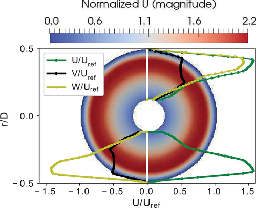
The swirl number based on the flux of momentum, omitting the pressure term (Lilley 1995), results in $S{ }^{\mathrm{\prime }}=0.7$ for the used inlet velocity profiles shown in Figure 2.

For the blunt swirler hub, we conduct simulations on two grids with variable resolution. The coarse numerical grid has 1.5 M cells, and the fine one has 2.5 M cells, where refinement is distributed equally in all directions. Both meshes fulfill the Pope criterion (Pope 2000). The turbulence conditions in the inflow duct containing the swirler are unknown and have to be estimated. We assume a turbulence intensity of $TI=15\mathrm{\%}$ at the inlet (downstream of the swirler) and specify a turbulence integral length scale of 1.9 mm at the simulated inlet, which corresponds to $10\mathrm{\%}$ of the step height $D/2=0.019\mathrm{m}$. A synthetic inflow turbulence generator, which is described by Kornev and Hassel (2006), is used to model the incoming turbulence. A comparison with parameters from Taamallah et al. (2019) is difficult, due to the different inlet conditions, but Taamallah et al. (2019) assumed a turbulence intensity of $5\mathrm{\%}$ an integral length scale of $19\mathrm{m}\mathrm{m}$ upstream of the swirler. For an instance of time in the developed flow, the spatial mean $y+$ for the first cell layer from the wall is $6.6$ for the coarse, and $6.1$ for the fine mesh. Turbulence wall functions applicable for low- and high-Reynolds number wall treatment are chosen to ensure correct flow behavior at the wall.

Simulations are carried out for two perfectly mixed lean methane-air mixtures (air-fuel equivalence ratios $\varphi =0.6,0.65$) with an inlet temperature of $300\mathrm{K}$. A Neumann boundary condition for temperature imposes adiabatic behavior at the wall. Besides Pope criterion, the degree of resolution of the flame is an important aspect of the mesh evaluation and is reflected by the scale ratio between cell size and flame thickness. For the lean combustion conditions investigated here, the laminar thermal flame thickness is ${\delta }_{\mathrm{t}\mathrm{h}}=1.1mm$ for $\varphi =0.6$ and ${\delta }_{\mathrm{t}\mathrm{h}}=0.8mm$ for $\varphi =0.65$. The minimum cell size for the 1.5 M mesh is 0.35 mm and the maximum cell size is 1.5 mm based on the cube-root of the respective cell volume, which is very similar to the resolution described by Taamallah et al. (2019). From this comparison, it can be expected that the flame brush will be partly resolved in some regions, especially for the lower equivalence ratio $\varphi =0.6$.

Results and discussion

Cold flow validation

Cold flow simulations are carried out first, to evaluate the suitability of numerical grid, turbulence model and boundary conditions, but also as a basis for the subsequent analysis of the influence of combustion on the flow field. Information on the inflow conditions to the burner from experiments is limited to the Reynolds number, bulk flow velocity and swirl number based on the geometry of the vanes. Hence, the subsequent careful cross-comparison with experimental data for mean and rms axial, radial, and tangential velocity data is of great importance to ensure suitable numerical settings for the reacting flow study. In addition to experimental data, simulation results are available from Taamallah et al. (2019) and Kewlani et al. (Kewlani, Shanbhogue, and Ghoniem 2016). to assess the performance of the current approach compared to other LES. Kewlani, Shanbhogue, and Ghoniem (2016) and Taamallah et al. (2019) included the swirler geometry in the computational grid, while in this study inflow profiles are defined at the axial location of the swirler outlet, conceptually located at the exit of the physical swirler outlet. Both this study and the study of Taamallah et al. (2019), used for comparison of cold flow data, applied a k-equation model for SGS closure in OpenFOAM. The different mesh and inlet conditions, especially the treatment of the swirling inflow, are expected to be important for differences in the results.

The focus of this study is on the region downstream of the expansion plane, where the primary flame is located and a comparison with experiments is able to underpin the confidence in our LES. No experimental data are available to back simulation results in the near field of the swirler, and it is well known that general statements on the structure of swirling flows are problematic due to the strong configuration dependence (Lieuwen 2012). Additionally, the interaction of cold/hot swirling flows with obstacles is complex (Kallifronas et al. 2022; Vanierschot and Van den Bulck 2008). Potential differences in the flow field within the swirler duct shall be addressed.

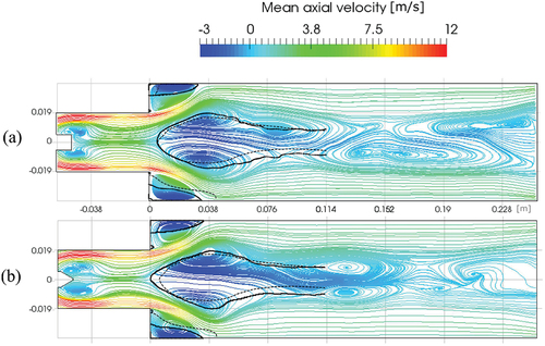
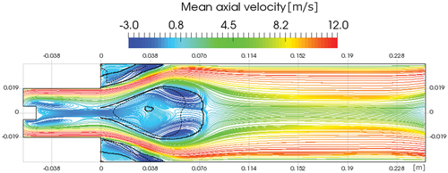
Figure 3 suggests that the flows evolving behind the two different swirler hubs show very similar statistics. The mean ORZ length downstream of the sudden duct expansion at $x=0$ is predicted to be around 0.9$D$ by both our simulations, as can be seen in Figure 3, where zero-isolines of the 2-d velocity magnitude (axial, radial), both for experiments and our simulations, are compared. From this, it becomes clear that the swirler hub shape will only minorly influence the outer recirculation zone. The experimental contours in Figure 3 show asymmetric behavior but provide a value for the larger ORZ length of approximately 1.05$D$, which indicates that our simulations reach good agreement with measurements. The most striking difference between the two presented cases is the comparatively broadened and elongated wake behind the conical swirler hub, which leads to a deflection of the swirling annular jet radially outward. This is reflected by a broader, high axial velocity jet region observable throughout the swirler duct and also at the entrance into the expansion duct. The coloring of streamlines with axial velocity also indicates that in the central far-field of the expansion duct, higher reversed flow velocities are observable for the blunt swirler hub simulation.

Figure 3. Mean flow streamlines for (a) blunt and (b) tapered swirler hub. Black zero-isolines of dimensional velocity magnitude (axial, radial) for presented cold flow simulations

, for experiments described in Taamallah et al. (2019)

.

Downstream of the expansion plane, along the centerline, an approximately axisymmetric vortex bubble is captured in the simulations as shown in Figure 3. The wakes directly downstream of the swirler hubs are predicted to be separate from the vortex bubbles, which depends on the swirl number, as was shown in a study by Kallifronas et al. (2022). The IRZ with tapered swirler hub applied has a mean stagnation point located in the expansion plane $x=0$ on the burner symmetry axis $r=0$, as seen in Figure 3. For the blunt centerbody, the time-averaged position of this stagnation point is located on the symmetry axis as well, slightly downstream of the expansion plane, which agrees well with measurements. Downstream of these stagnation points, the tip regions for both vortex bubbles form an angle of roughly ${45}^{\circ }$ to the streamwise direction, their low-velocity tails are of similar width. The predicted shapes agree well with experiments for both conditions, as shown in Figure 3. The tails of both recirculating bubbles show to a varying degree symmetric behavior. For a more detailed discussion of the mean flow structures, 3-d streamlines based on the time-averaged velocity are presented for the core region in Figure 4.

Figure 4. 3-d mean flow streamlines for (a) blunt and (b) tapered swirler hub. Streamlines in green capture the predicted centermost structure of the IRZ, streamlines in blue the flow around the vortex bubble. Orange streamlines show a helical filament wrapped around the inner region.

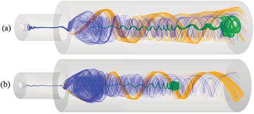
Figures 4a,b show vortical motions extracted from mean velocity data for a better visualization and understanding of the flow. Streamlines colored in green capture the predicted centermost structure of the IRZ, where transport of material into the front part of the vortex bubble in counter-clockwise rotation, considering the direction of flow, is observed. Rotating in opposite direction, in accordance with the swirler-induced motion, the blue streamlines capture the predicted flow around the vortex bubble. Wrapped around these structures is a helical filament (orange streamlines). Although colored in green and orange for better distinction, both vortical structures are connected through continuous streamlines, indicating that the helical filament is linked to the recirculating flow through the inner region of the bubble. The main visible difference between the two investigated cases for a blunt and tapered swirler hub is the downstream structure of the recirculating bubble tail involved in the transport of material upstream. For Figure 4a it forms a bundle of streaks, while for Figure 4b it shows an organized structure further upstream. For the blunt swirler hub, the flow around the IRZ is observed to spread radially outward leading to the broadening of the tail downstream. A slight compression effect both radial and longitudinal was observed for the tapered swirler hub. Clearly, changing the shape of the swirler hub has a profound effect on the structure and behavior of the vortex bubble and the spatial subsequent evolution of the flow.

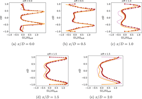
Normalized mean axial velocity variations in the radial direction are shown in Figure 5 for different axial locations. The first experimental data set (Figure 5a) is available for the expansion plane. We collect data for this plane one cell layer away from $x=0$, to capture the flow close to the vertical step wall.

Figure 5. Normalised mean axial velocity in radial direction for the cold flow. Orange solid lines

and light green dashed lines

denote the current results using the 1.5 M and 2.5 M mesh with blunt swirler hub. Blue dash-dotted lines

provide results for the case with tapered swirler hub on a 1.5 M mesh. The magenta dotted lines

denote simulation results from Taamallah et al. (2019) and the dark red dots

connected by dashed lines are respective experimental results from Taamallah et al. (2019).

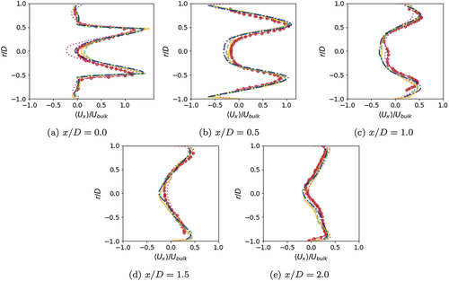
In Figure 5, simulation results are plotted for the blunt (orange solid lines) and tapered swirler hub (green dashed lines) on the 1.5 M cells meshes. They are shown together with results for the blunt swirler hub on a 2.5 M mesh (blue dash-dotted lines) and measurements and LES results from Taamallah et al. (2019). Overall, a good agreement can be observed between the different numerical set-ups and approaches compared here, and the ability to capture the measured flow field is very similar for them. Locally, some quantitative differences exist, most prominently in the IRZ, which is expected to be sensitive to even minor changes in the swirling flow conditions caused, e.g., by the different choice of inlet conditions. The comparison of cases with varying resolution (1.5 M, 2.5 M cells) in Figure 5 does not show a considerable merit achieved through grid refinement, which is why only the 1.5 M cells case will be investigated further. Figures A3 and A1, provided in Appendix A, complement the evaluation of mean flow fields for the cold case and indicate good agreement between our simulations, experiments and simulations from Taamallah et al. (2019) also for radial and tangential velocity components.

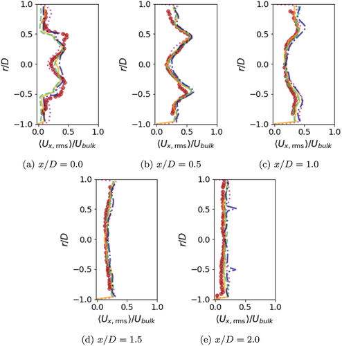
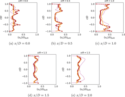
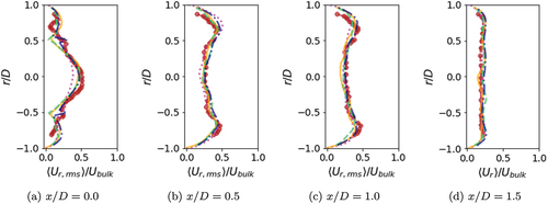
Next, the root-mean-square (rms) velocity variations given in Figure 6, as well as Figures A2 and A4, are considered. The rms velocities in LES consist of a resolved part $⟨U^2-⟨U{⟩}^2⟩$ and a subgrid-scale component. In this study, the SGS contribution $u{{ }^{\mathrm{\prime }}}_{\mathrm{s}\mathrm{g}\mathrm{s}}$ is approximated and included using the relation $⟨k_{\mathrm{S}\mathrm{G}\mathrm{S}}⟩=3/2⟨u{{ }^{\mathrm{\prime }}}^2⟩$. The same applies also to the radial component $u{{ }^{\mathrm{\prime }}}_{\mathrm{s}\mathrm{g}\mathrm{s}}\approx v{{ }^{\mathrm{\prime }}}_{\mathrm{s}\mathrm{g}\mathrm{s}}$. The rms velocity variations agree well with experimental data. The results of the cold flow underpin the ability of the computational setup, in terms of boundary and inlet conditions, turbulence model and grid, to capture the characteristics of the flow. Very good comparisons with the measured flow field and structures are achieved, despite excluding the swirler geometry in the computational model, and this gives confidence using this computational setup for reacting flow simulations.

Figure 6. Normalized rms axial velocity variation in radial direction, for legend see Fig. 5.

The mean fields of the cold flow show subtle differences in the far-field for the two swirler hubs investigated here. The structure and velocity magnitude of the center vortex tail shows some discrepancies for both cases. At first glance, it seems paradoxical that the blunt swirler hub case shows slightly better agreement with measurements than the tapered one, especially when it comes to the position and shape of the bubble in the expansion duct. Two aspects influencing this behavior are described in the following; however, swirling flows are highly complex (Lieuwen 2012). First, the shape of the swirler hub has a strong influence on the velocity and pressure field and, thereby, also affects the swirl number. The degree of swirl is known to be an important parameter controlling the flow evolution and development of its structure through instabilities (Lieuwen 2012). The experiments provided only a geometric swirl number based on the vane angle and were not based on the ratio of axial to azimuthal momentum fluxes in the axial direction. Second, the inlet velocity profiles used here and documented by Lilley (1995) are measured upstream of a blunt swirler hub and, due to the formation of wake, it is possible that also the upstream flow field is influenced by the shape of the swirler hub. Unfortunately, the lack of measurements in the swirler duct poses challenges to find the actual reasons for the observed sensitivities. We would like to appeal to the experimentalists to characterize the attributes of the incoming flow clearly for future experiments.

Flame shape and local extinction

Shanbhogue et al. (2016) hypothesized that the flame shape is controlled by the ability of the flame to sustain in regions of high strain and showed that a correlation between extinction strain rate and presence of the flame in the OSL and the ORZ exists. They further observed that for higher equivalence ratio, and thus higher extinction strain rate, the flame was able to propagate from the ISL into the ORZ, establishing also in the OSL. Taamallah et al. (2019) and Kewlani et al. (Kewlani, Shanbhogue, and Ghoniem 2016). studied two flames with varying equivalence ratio $\varphi =0.6$ and $\varphi =0.65$, referred to as Flame III and IV, closely using particle image velocimetry (PIV). It was observed that Flame III was located in the ISL, while Flame IV was able to sustain also in the OSL, corresponding to a transition from a $V$-shaped to an $M$-shaped flame (Kewlani, Shanbhogue, and Ghoniem 2016). Both flames were measured, as well as simulated using LES with the Thickened flame model in earlier studies (Kewlani, Shanbhogue, and Ghoniem 2016; Taamallah et al. 2019), mean and rms velocity data for the axial and radial component $U,V$ are available for cross-comparison. Moreover, details on the flame shape, shear layers and dynamic behavior of the flame are available through a number of past studies using this burner (Kewlani, Shanbhogue, and Ghoniem 2016; Shanbhogue et al. 2016; Taamallah et al. 2014, 2015, 2019; Taamallah, Shanbhogue, and Ghoniem 2016). For the considered configuration, Taamallah et al. (2015) investigated the effect of thermal boundary conditions on the flame shape and concluded that the transition remained unaffected by the heat transfer through the wall when the ORZ was initially cold. However, thermal boundary conditions became important once the ORZ was ignited.

Before presenting the results for Flames III and IV, the extinction model from Section 3.1 is clarified further. More specifically, the chemical timescale, and its relevance to local extinction through high turbulence stretch has to be addressed. Shanbhogue et al. (2016) observed a strong relation between extinction strain rates ${\kappa }_{\mathrm{e}\mathrm{x}\mathrm{t}}$ calculated using opposed-jet laminar twin flames and the local flow conditions and flame shapes in their experimental studies. Shanbhogue et al. (2016) further noted that for extinction strain rates in the range $256{\mathrm{s}}^{-1}<{\kappa }_{\mathrm{e}\mathrm{x}\mathrm{t}}<522{\mathrm{s}}^{-1}$ the flame stabilized in the ISL, and for ${\kappa }_{\mathrm{e}\mathrm{x}\mathrm{t}}>572{\mathrm{s}}^{-}1$ the flame moved to the ORZ. We use the flame transit time $D_{\mathrm{r}}/(S_{\mathrm{u},0}^2)$ for the laminar premixed flame as the representative chemical timescale, which is ${\tau }_{\mathrm{c}}={\tau }_{\mathrm{t}\mathrm{r}\mathrm{a}\mathrm{n}\mathrm{s}}=1.6\times {10}^{-3}\mathrm{s}$ for $\varphi =0.6$ and ${\tau }_{\mathrm{c}}={\tau }_{\mathrm{t}\mathrm{r}\mathrm{a}\mathrm{n}\mathrm{s}}=9.2\times {10}^{-4}\mathrm{s}$ for $\varphi =0.65$. For the laminar premixed flame calculations carried out in Cantera (Goodwin et al. 2015), the GRI-Mech 3.0 (Smith et al. n. d.) chemical mechanism was used. The flame transit times calculated are of similar order of magnitude as the extinction time scales used by Shanbhogue et al. (2016) and are linked to the inner reacting structure. The performance of this approach will be discussed in the following sections. For comparison, also a chemical timescale $t_c=\rho /{\dot{\omega }}_{c,max}\ll D_{\mathrm{r}}/(S_{\mathrm{u},0}^2)$ based on the local maximum reaction rate of the laminar flame is tested. Using this formulation, the quenching of the flame by high stretch is not captured due to $t_c$ being much smaller than the local SGS turbulence time scales. Hence, this approach is not included in detail in this study.

Flame III validation

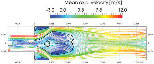
The flow field for Flame III shown in Figure 7 has undergone considerable changes compared to the cold flow in Figure 3 due to the heat release from the combustion. In Figure 7, the isolines of zero 2-d velocity magnitude (axial, radial) are shown for our simulation together with measurements of the IRZ and ORZ from Taamallah et al. (2019) and streamlines based on our time-averaged 2-d velocity data colored by the axial velocity component. The flow field of the reacting case in Figure 3 is characterized by higher axial velocities due to thermal expansion of the burnt gas, which affects the swirl number. Naturally, the most striking change in the flow structure between cold flow and Flame III is connected to the recirculation bubble. The wake behind the swirler hub and the IRZ downstream of the expansion plane grow together for Flame III, while the tail of the IRZ disappears. This was also observed in the numerical study of Taamallah et al. (2019) and was indicated by experiments as the stagnation point at $x/D=0$ clearly moved upstream. Analyzing the IRZ, our simulation results suggest that the recirculating bubble consists of a vortex ring with negative inside axial velocities. At its heart-shaped end downstream, our simulation predicts the presence of an, on-the-mean, spirally shaped structure rotating clockwise in the flow direction. We connect this structure to the transport of hot material into the IRZ. The predicted IRZ shows a second, smaller vortex located roughly on the symmetry axis, transporting material, on-the-mean, in the opposite axial direction to the outer ring structure. The approximately circular, zero velocity isoline in Figure 7 indicates an axisymmetric region smaller $D/2$ of positive axial velocity predicted by our simulation, which is located between $x/D=0.5$ and $x/D=1$. Experiments captured a region of positive axial flow of almost $2D$ length located slightly off the burner symmetry axis within the IRZ, which is observable in Figure 7. This vortical structure has a droplet form and its tip reaches close to the downstream stagnation point of the IRZ in experiments. The agreement is good for both the inner vortical structure and the vortex ring, the length of the IRZ is overestimated by the simulation by less than $0.5D$. The ORZ remains unignited for the V-shaped Flame III, hence its shape does not change considerably in Flame III. It is predicted by our simulations for the cold flow to be slightly shorter than $1D$, while for Flame III it is shown to be marginally larger than $1D$.

Figure 7. 2-d streamlines colored by mean axial velocity for the hot flow with air-fuel equivalence ratio $\varphi =0.6$. Black lines are contours of zero 2-d (axial and radial) velocity from the simulation of flame III

and measurements (Taamallah et al. 2019)

.

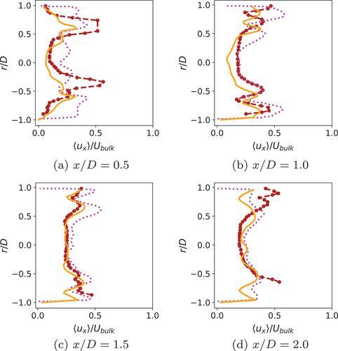
The velocity profiles for Flame III are given in Figure 8. The measured peak velocities are capture well in the simulation. Compared to the cold flow, the axial peak velocities are predicted to be considerably higher in Flame III due to dilatation effects, downstream of $x/D=1.0$ almost twice as large. It is clear that the mean axial velocity profile in the IRZ has two inflection points forming a W-shape. This behavior is due to the positive axial flow setting in between $x/D=0.5$ and $x/D=1.0$, where the secondary vortex within the IRZ is located. The prediction of the statistics of the vortex bubble is excellent for $x/D<1.0$ and very good for further downstream locations shown in the figure. The discrepancy between the experimental tear-drop shaped inner vortex and the almost circular one from the simulation is notable. In addition to the axial velocity profiles, more validation data are given in the attachment in Appendix B and the comparisons seen in these figures are also very good.

Figure 8. Normalised mean axial velocity profiles in radial direction for flame III with air-fuel equivalence ratio $\varphi =0.6$. Orange solid lines

denote the current results using the 1.5 M mesh. The magenta dotted lines

denote simulation results from Taamallah et al. (2019) and the dark red dots (

) connected by dashed lines are respective experimental results from Taamallah et al. (2019).

It is notable in Figure 9 through distinct peaks in the rms velocity profiles that the flame generates strong turbulence in the ISL. In contrast, the low-velocity fluctuations inside the IRZ suggest that the bubble itself is very stable. The agreement of the current computational results with experimental data is good throughout the measurement region. The lack of measured wall temperatures poses uncertainty for the wall thermal boundary condition and hence this leads to some differences between the measured and computed rms velocities in the near-wall regions. However, the V-shaped flame remains largely unaffected by these local uncertainties due to its stabilization at a distance from the wall in the shear layers between the swirling annular jet and IRZ. Finally, we shall compare our results for Flame III with an LES using the Thickened flame model (Taamallah et al. 2019). The flow statistics for Flame III show clearly that the modeling approach in this study exhibits improved performance to predict the mean structures of IRZ, ORZ, and shear layers, qualitatively and quantitatively. More pronounced deviations between the numerical studies of Flame III compared to the cold flow underpin that the combustion closure controls the modeling performance in hot flows.

Figure 9. Normalized rms axial velocity variation in radial direction for flame III, for legend see Figure 7.

Flame IV validation

For Flame III, it is shown that the heat release has a considerable impact on the flow field. Flame IV (Kewlani, Shanbhogue, and Ghoniem 2016) is operated at a lean equivalence ratio of $\varphi =0.65$, which results in an increased heat load compared to Flame III. In Figure 10, streamlines based on the 2-d mean velocity field colored by the mean axial velocity magnitude, and isolines of zero velocity are shown for the simulations and experiments. The influence of the increased heat release on the axial velocity field in Flame IV can be seen comparing the high axial-velocity regions colored in red in Figure 10 with those in Figure 7. For Flame IV, broader regions of the flow undergo acceleration due to thermal expansion. The agreement between experiment and simulation deteriorates slightly for this case compared to Flame III. This is notable from the deviation between the measured and predicted shape and position of the ORZ and IRZ for this simulation (Figure 10) as well as the LES from Kewlani, Shanbhogue, and Ghoniem (2016). In experiments (Kewlani, Shanbhogue, and Ghoniem 2016), a separation of the vortex bubble and the wake behind the swirler hub is documented for Flame IV as the IRZ undergoes a considerable decrease in size compared to the cold flow and Flame III. However, the measurements for Flame IV face uncertainties concerning the flow structures. The measured breakdown bubble for Flame IV (Watanabe et al. 2016) shows an IRZ reaching upstream into the inlet duct and a secondary vortex of positive axial flow within it.

Figure 10. 2-d streamlines colored by mean axial velocity for the hot flow with air-fuel equivalence ratio $\varphi =0.65$. Black zero-isolines of 2-d velocity magnitude (axial, radial) for simulation

and measurements described in Taamallah et al. (2019)

.

For the simulation, we observe a tapering of the connection between the vortex bubble and the wake behind the swirler hub, but no complete separation of the two structures. Furthermore, a radial contraction of the vortex bubble compared to Flame III is predicted by the simulation in agreement with experiments, whereas its length is overestimated by around $0.5D$. The ORZ, delimited radially inward by the zero velocity isoline, is overpredicted by around $25\mathrm{\%}$ in the simulation. The comparison of Flame III and Flame IV reveals that the zero velocity isoline, confining the outer recirculation zone, moves closer to the annular swirling jet in Flame IV, both for experiments and simulations. The recirculation zone length does not change considerably for Flame IV and is around $1.2D$ for the simulation, while it remained almost unchanged at $x/D=1$ in the experiments, as shown in Figure 10. The V-shaped flame simulations have also been carried out varying ${\beta }^{\prime }$ to investigate the impact of this parameter. It is observable that increasing ${\beta }^{\prime }$, the flame is eventually able to reach the corner recirculation zones. One reason for this behavior is potentially the strong coupling between the turbulent flame speed and the scalar dissipation rate of the progress variable $c$, as well as the turbulent reaction rate. This idea is supported by the literature, for example Kolla et al. (2009). The lack of information on the turbulent flame speed makes a dependable discussion of this observation difficult for this setup. Future work will have to look into this relation. For the subsequent analysis, the value for ${\beta }^{\prime }$ is chosen based on the considerations outlined in the model description of this study.

For the evaluation of the modeling results for Flame IV, rms and mean axial velocities are available from measurements and an LES (Kewlani, Shanbhogue, and Ghoniem 2016). Velocity variations are shown in Figures 11 and 12. The mean variations show good quantitative agreement between the predicted and measured normalized peak velocities. A notable asymmetry in the velocity measurements in Figure 11a is observable. In the negative $r/R$-range the agreement between the presented simulation and experimental results is very good, but stronger deviations are observed in the positive range. The rms-velocity variations for the simulation and experiments match well, however, the two broad peaks of axial rms-velocity associated with the ISL and OSL at $x/D=0.5$ are considerably underpredicted by the presented simulation. Further downstream, the agreement improves again and it is not fully clear what causes the considerable deviation in this axial location. In direct comparison with modeling data from Kewlani, Shanbhogue, and Ghoniem (2016), the presented simulation achieved competitive performance and a slightly better agreement with experiments for the rms velocity variations. Overall, the validation demonstrates the suitability of the LES to reflect the behavior of the flame. In the following, we will study the flame structure in detail.

Figure 11. Normalized mean axial velocity profiles in radial direction for flame IV. Orange solid lines

denote the current results using the 1.5M mesh. The magenta dotted lines

denote simulation results from Kewlani, Shanbhogue, and Ghoniem (2016) and the dark red dots (

) connected by dashed lines are respective experimental results from Kewlani, Shanbhogue, and Ghoniem (2016).

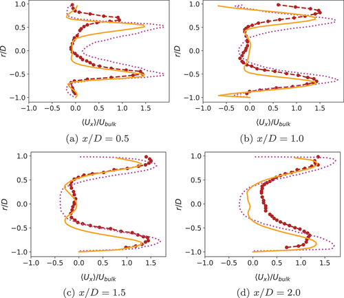
Figure 12. Normalized rms axial velocity variation in radial direction for flame IV, for legend see Figure 11.

Analysis of flame shape

The normalized mean reaction rate shown in Figure 13 depicts the difference in flame shapes between Flames III and IV. Flame III (Figure 13a) is located in the ISL between IRZ and swirling annular jet, and no reactions are observed in the OSL and ORZ, which is consistent with the experimental observations and the results of past LES studies (Taamallah et al. 2019). A point measurement of temperature (TC1) for this case in the ORZ $10\mathrm{m}\mathrm{m}$ downstream of the expansion plane and $5\mathrm{m}\mathrm{m}$ away from the burner side wall using a thermocouple was provided by Taamallah et al. (2019) to assess the reacting conditions in the ORZ. The experimental measurement gave a temperature of $410\pm 5\mathrm{K}$. In our simulation, the temperature is approximately $391\mathrm{K}$, the LES of Taamallah et al. (2019) gave a temperature of $423\mathrm{K}$. Both predictions of TC1 lie slightly outside the experimental measurement uncertainty with a deviation of less than $25\mathrm{K}$ and $20\mathrm{K}$, respectively.

Figure 13. Normalized (nondimensional) mean reaction rate $〈{\overline{\dot{\omega }}}_{\text{c}}〉{\delta }_{\text{th}}/({\rho }_{\text{u}}{S}_{\text{L},\text{0}})$ for (a) Flame III resulting in a V-shaped flame and (b) Flame IV resulting in an M-shaped flame.

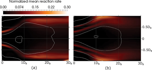
Intense reactions for the V-shaped flame are observed along the duct, at small distances from the wall from $1D$ downstream of the expansion plane for the simulation, which agrees well with experimental measurements using the optical diagnostic tools OH-Planar Laser-Induced Fluorescence and Chemiluminescence (Taamallah et al. 2015). The intensifying of reactions can be explained by the increased mixing between fresh and burnt gases after the swirling annular jet impinges the wall. A considerable broadening of the mean reaction zone is also observed downstream of this point. Two thin, shear-layer stabilized flames are seen for the M-shaped Flame IV, with a strong reaction intensity in the OSL flame branch close to the wall impingement point shown in Figure 13b. Flame IV is considerably shorter than Flame III with the highest mean reaction rates between $1-2D$ and a quick fading out of reaction activity for the region around $3D$ in axial direction. The mean flame structure of Flame IV predicted by simulation agrees also well with the behavior observed in experiments for this flame (Taamallah et al. 2015). Microstructures and instantaneous flow fields will be investigated subsequently.

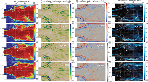
Figure 14 gives an idea of the flame micro structures and filtered, instantaneous fields for Flame III. It provides midplane cuts through the expansion duct showing filtered progress variable, normalized strain rate magnitude, out-of-plane vorticity and reaction rate for four different instants of time with a time lag of $\mathrm{\Delta }t=1\mathrm{m}\mathrm{s}$. In correspondence with experimental studies of Flame III (Taamallah, Shanbhogue, and Ghoniem 2016), the simulation predicts that reacting structures are located along the ISL and rolled up by vortical structures as a consequence of their hydrodynamical instability. The first column of Figure 14 shows the filtered progress variable field for the four time steps and shows a strong wrinkling of the flame structure with the onset of pocket formation. For better visualization, one such wrinkled reacting structure is marked using a white dashed circle in the first column of Figure 14 displaying the progress variable field. The second column captures the position of shear layers as streaks of high strain rate magnitude. The isolines of progress variable of $c=0.1$ and $c=0.5$, shown in magenta, are plotted and indicate the location of the filtered flame. They confirm the presence of the flame in the thin region between the vortex bubble and the swirling annular jet. The vorticity field, displayed in column three, together with c-isolines and zero-axial velocity isolines (white lines) uncovers the presence of vortices in the shear layers, relating the flame wrinkling to roll-up phenomena in the unstable ISL. One such vortex, which is marked with a white dashed circle in Figure 14 first column, wrinkles the flame notably in the shown time sequence. For an equivalence ratio of $\varphi =0.6$, it has a core radius in the order of two to three times the laminar flame thickness. The inner high vorticity regions are characterized by a rotation clockwise in positive and anti-clockwise in negative radial direction. Taamallah et al. (2015) observed experimentally that wrinkles of up to $8\mathrm{m}\mathrm{m}$ diameter or approximately $D/5$ occurred. At $t_0$ the vortex is visible on the burnt side with an intact flame. This vortex subsequently entrains fresh gas into hot products and the evolution of this process can be seen in the first column of Figure 14. The vortices in the ISL draw the flame away from the ORZ. The vortices in the OSL counter-rotate and hence transport material toward the duct wall and ORZ. The 2-d streamlines displayed in Figure 14 indicate a complex interaction of the vortical structures in the ISL, OSL and ORZ. The vortices in the shear layers are organized in a zigzag pattern, an indication for aligned roll-up of the ISL and OSL. The corner region in the positive radial direction shows the interaction of the primary eddy in the ORZ with a considerably stronger vortex in the OSL. The visible, intense anti-clockwise vorticity in the OSL coincides with the presence of reacting material in the ORZ, temporarily leading to reactions in parts of the ORZ. This is visible from the fourth column of Figure 14 displaying the normalized reaction rate. In this filtered reaction rate, both the individual contributions of the resolved and SGS term enter, which were investigated to be of similar order of magnitude in the reaction zones. This confirms the initial hypothesis that due to the resolution of the grid $\mathrm{\Delta }/{\delta }_{\mathrm{t}\mathrm{h}}\approx 1$, a two term formulation considering the resolved scales is beneficial. From the different mechanisms that are known to cause flashback in premixed flames (Fritz, Kröner, and Sattelmayer 2004), the observed transport of hot material with vortices emerging from the OSL can be considered as flashback due to combustion instabilities. This phenomenon has also been observed experimentally by Taamallah et al. (2015), by extracting flame intensities from high-speed images of the flame close to the shape transition.

Figure 14. Midplane cut through the expansion duct with filtered progress variable, normalized strain rate magnitude $S_{\mathrm{N}}=\parallel S_{ij}\parallel D/U_{\mathrm{r}\mathrm{e}\mathrm{f}}$, out-of-plane vorticity ${\omega }_{\mathrm{N}}={\omega }_{z}D/U_{\mathrm{r}\mathrm{e}\mathrm{f}}$ and reaction rate $⟨{\dot{\omega }}_{\mathrm{c}}⟩{\delta }_{\mathrm{t}\mathrm{h}}/({\rho }_{\mathrm{u}}{S}_{\mathrm{L},0})$ for equivalence ratio $\varphi =0.6$ displayed, all shown quantities are nondimensional.

The entrainment occurs where the reacted material comes close to the ORZ and enters the sphere of influence of strong OSL vortices. This corresponds to the region of impingement and breakdown of the swirling annular jet at the wall. It should be noted that the wall temperatures are comparatively low during the described process of hot-gas entrainment into the ORZ for the V-shaped flame, both in our simulations and experiments (Taamallah et al. 2015). Taamallah et al. (2015) showed that varying the wall heat losses did neither influence the wall temperatures nor the equivalence ratio at which the flame transitioned from V-shape to M-shape considerably. From this observation, they hypothesized that the flame in the investigated burner configuration was weakly influenced by the wall thermal boundary condition as long as it was not established in the ORZ. The results of our simulations support this hypothesis. Based on the analysis above, there is strong evidence that for this configuration, the interaction of the unignited ORZ with the flame happens dominantly through the exchange of hot fluid with the ISL, caused by strong vortices of the unstable OSL, rather than through interaction of the flame with the wall. An important aspect of this behavior might be that the important mechanism of boundary layer flashback, which is strongly affected by the interaction of the flame with the wall, has neither been documented by Taamallah et al. (2015) nor has been observed in our simulations. The strong velocity gradients, where the annular jet impinges the wall, appear to prevent the creeping of the flame upstream into the ORZ (Fritz, Kröner, and Sattelmayer 2004) within the boundary layer.

The impingement and swirling annular jet breakdown is concurrently characterized by high strain rates in our simulation. The ability of the OSL vortices to deflect hot material from its downstream movement is expected to depend on the presence of hot material and hence the location of the flame in this region of high strain. In this region, turbulence time scales compete with chemical ones, the investigated condition for the onset of local extinction. From the normalized reaction rate fields provided in the fourth column of Figure 14 it is observed that intense reacting structures stay away from the outer shear layer and recirculation zone. This agrees with observations of Taamallah, Shanbhogue, and Ghoniem (2016), who connected the transition to an M-shaped flame with a threshold value for the ratio between the large-scale flow time of the ORZ (spinning frequency) and the extinction timescale implying that both processes, entrainment, and supply of hot material, were important for the V- to M-flame transition in this burner.

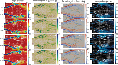
Finally, we investigate a time sequence of fields for the M-shaped flame to study the main differences to the V-shaped flame. For this case, we observe reacting structures both along the inner and outer shear layer, which can be seen in the figures in the first and second columns in Figure 15, showing the filtered progress variable and strain rate magnitude with progress variable isolines for $c=0.1$ and $c=0.5$ superimposed. This shape agrees with measurements (Kewlani, Shanbhogue, and Ghoniem 2016; Taamallah et al. 2015). In our simulation, the unstable shear layers undergo also for this case roll-up, which becomes clear from the vorticity fields that are shown in column three. This leads to a wrinkling of the flame surface as represented by progress variable isolines for $c=0.1$ and $0.5$ superimposed on the vorticity fields. It should be noted that the flame sheet in the ISL, especially in the region $x/D<1.0$, shows only minor deformation, indicating a transition in flame structure for the ISL compared to the leaner Flame III. The interface between cold swirling annular jet and corner flow is characterized by the presence of intense vorticity and a wrinkled flame is present in the OSL. Compared to Flame III, the high vorticity streaks in the OSL appear thickened in the presence of the flame. The zero-axial velocity isoline for Flame IV suggests a much larger recirculation zone located close to the OSL while inside the corner region, a considerably decreased vorticity is observable.

Figure 15. Midplane cut through the expansion duct with filtered progress variable, normalized strain rate magnitude $S_{\mathrm{N}}=\parallel S_{ij}\parallel D/U_{\mathrm{r}\mathrm{e}\mathrm{f}}$, out-of-plane vorticity ${\omega }_{\mathrm{N}}={\omega }_{z}D/U_{\mathrm{r}\mathrm{e}\mathrm{f}}$ and reaction rate $⟨{\dot{\omega }}_{\mathrm{c}}⟩{\delta }_{\mathrm{t}\mathrm{h}}/({\rho }_{\mathrm{u}}{S}_{\mathrm{L},0})$ for equivalence ratio $\varphi =0.65$ displayed, all shown quantities are nondimensional.

Conclusions

This study considers two swirl-stabilized premixed turbulent flames with different lean equivalence ratio forming a V- and M-shape, respectively. Predefined inlet profiles based on detailed measurements are used to model the swirling inflow. Our cold flow results show that these predefined inlet profiles are adequate to capture the measured flow field, suggesting that the swirler geometry may not have to be included in the computations, at least for the cases investigated here. Including the swirler geometry can increase the computational cost substantially. However, one must have experimentally well-characterized flow field at the swirler exit. We investigate the influence of two different swirler hubs and observe minor differences for the main statistics (mean and rms velocity components) in the far-field of the swirler under non-reacting conditions. However, we observe that the macrostructures of the flow are influenced by the choice of swirler hub, and the reasons for the observed behavior are discussed.

The computational results compare well with measurements for two flames, Flame III (V-shaped) and IV (M-shaped). These results indicate that the flow-combustion coupling is well captured by the modeling approach used for this study. The current LES results also agree well with past computational results for these flames (Kewlani et al. 2016; Taamallah et al. 2019). The combustion closure used in this study is a modified version of a dissipation based reaction rate model first presented by Tomasch et al. (2022), which includes local finite-rate chemistry effects. Hence, local extinction arising from finite-rate chemistry effects can be captured using this subgrid reaction rate model. The main features of V- and M-shaped flames observed experimentally are captured well using this combustion model. A qualitative comparison with OH-PLIF and chemiluminescence, e.g. (Taamallah et al. 2015) shows good agreement in terms of the position of flame, intense reacting regions, and the expected flame length. The LES results are analyzed to provide insights on the stabilization mechanisms of these flames. The structures of ORZ and IRZ, the vorticity strength in these regions compared to the shear and the location of the shear layers control the flame shape in this burner configuration.

Disclosure statement

No potential conflict of interest was reported by the author(s).

Additional information

Funding

The work has been funded by the Norwegian Research council, Climit programme, project No. 268368, OxyFun Fundamentals of pressurized oxy/fuel combustion. The simulations were performed on resources provided by Sigma2 - the National Infrastructure for High Performance Computing and Data Storage in Norway (project No. NN9400K).

Appendix A.

Additional cold flow velocity data

Figure A1. Normalized mean tangential velocity profiles in radial direction for the cold flow, for legend see Fig. 5.

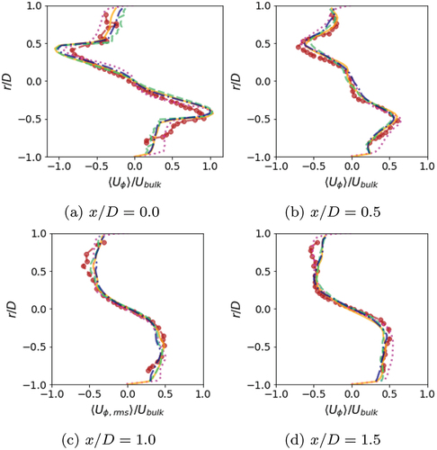
Figure A2. Normalized rms tangential velocity variation in radial direction for the cold flow, for legend see Fig. 5.

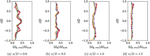
Figure A3. Normalized mean radial velocity profiles in radial direction for the cold flow, for legend see Fig. 5.

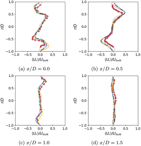
Figure A4. Normalized rms radial velocity variation in radial direction for the cold flow, for legend see Fig. 5.

Appendix B.

Additional Flame III velocity data

Figure B1. Normalized mean radial velocity profiles in radial direction for flame III, for legend see Fig. 8.

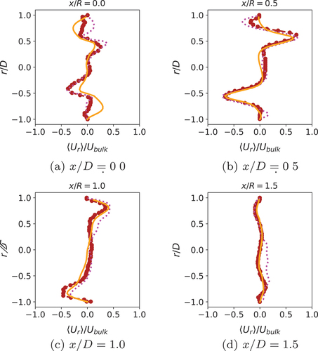
Figure B2. Normalized rms radial velocity variation in radial direction for flame III, for legend see Fig. 5.

References

- Bray, K. N. C. 1979. The interaction between turbulence and combustion. Symp. Combust. Proc 17 (1):223–33. doi:10.1016/S0082-0784(79)80024-7.
- Bray, K. N. C. 2011. Modelling Methods, book section 2, 41–150. Cambridge, UK: Cambridge University Press.
- Bray, K., M. Champion, and P. A. Libby. 2010. Systematically reduced rate mechanisms and presumed PDF models for premixed turbulent combustion. Combust. Flame 157 (3):455–64. doi:10.1016/j.combustflame.2009.09.017.
- Chakraborty, N., and N. Swaminathan. 2011. Effects of lewis number on scalar variance transport in premixed flames. Flow Turbul. Combust. 87 (2):261–92. doi:10.1007/s10494-010-9305-0.
- Chen, Z. X., I. Langella, R. S. Barlow, and N. Swaminathan. 2020. Prediction of local extinctions in piloted jet flames with inhomogeneous inlets using unstrained flamelets. Combust. Flame 212:415–32. doi:10.1016/j.combustflame.2019.11.007.
- Dunn, M. J., A. R. Masri, and R. W. Bilger. 2007. A new piloted premixed jet burner to study strong finite-rate chemistry effects. Combust. Flame 151 (1):46–60. doi:10.1016/j.combustflame.2007.05.010.
- Dunstan, T. D., Y. Minamoto, N. Chakraborty, and N. Swaminathan. 2013. Scalar dissipation rate modelling for large eddy simulation of turbulent premixed flames. Proc. Combust. Inst. 34 (1):1193–201. doi:10.1016/j.proci.2012.06.143.
- Fritz, J., M. Kröner, and T. Sattelmayer. 2004. Flashback in a swirl burner with cylindrical premixing zone. J. Eng. Gas Turbines Power 126 (2):276–83. doi:10.1115/1.1473155.
- Galpin, J., A. Naudin, L. Vervisch, C. Angelberger, O. Colin, and P. Domingo. 2008. Large-eddy simulation of a fuel-lean premixed turbulent swirl-burner. Combust. Flame 155 (1):247–66. doi:10.1016/j.combustflame.2008.04.004.
- Gao, Y., N. Chakraborty, and N. Swaminathan. 2014. Algebraic closure of scalar dissipation rate for large eddy simulations of turbulent premixed combustion. Combust. Sci. Tech. 186 (10–11):1309–37. doi:10.1080/00102202.2014.934581.
- Goodwin, G., D. Mofat, K. Speth, and H. Raymond. 2015. Cantera: An object-oriented software toolkit for chemical kinetics, thermodynamics, and transport processes. Version 2.4.0. https://www.cantera.org
- Guiberti, T. F., D. Durox, P. Scouflaire, and T. Schuller. 2015. Impact of heat loss and hydrogen enrichment on the shape of confined swirling flames. Proc. Combust. Inst. 35 (2):1385–92. doi:10.1016/j.proci.2014.06.016.
- Guo, S., J. Wang, W. Zhang, B. Lin, Y. Wu, S. Yu, G. Li, Z. Hu, and Z. Huang. 2019. Investigation on bluff-body and swirl stabilized flames near lean blowoff with PIV/PLIF measurements and LES modelling. Appl. Therm. Eng. 160:1–13. doi:10.1016/j.applthermaleng.2019.114021.
- Kallifronas, D. P., P. Ahmed, J. C. Massey, M. Talibi, A. Ducci, R. Balachandran, N. Swaminathan, and K. N. C. Bray. 2022. Influences of heat release, blockage ratio and swirl on the recirculation zone behind a bluff body. Combust. Sci. Tech. 1–25. doi:10.1080/00102202.2022.2041616.
- Kewlani, G., S. Shanbhogue, and A. Ghoniem. 2016. Investigations into the impact of the equivalence ratio on turbulent premixed combustion using particle image velocimetry and large eddy simulation techniques: V and M flame configurations in a swirl combustor. Energy. Fuels 30 (4):3451–62. doi:10.1021/acs.energyfuels.5b02921.
- Kolla, H., J. W. Rogerson, N. Chakraborty, and N. Swaminathan. 2009. Scalar dissipation rate modeling and its validation. Combust. Sci. Tech. 181 (3):518–35. doi:10.1080/00102200802612419.
- Kornev, N. V., and E. Hassel. 2006. Method of random spots for generation of synthetic turbulent fields with prescribed autocorrelation functions. Comm. Numer. Meth. Eng 23 (1):35–43. doi:10.1002/cnm.880.
- Krikunova, A. I. 2019. M-shaped flame dynamics. Phys. Fluids 31 (12):1–9. doi:10.1063/1.5129250.
- Langella, I., J. Heinze, T. Behrendt, L. Voigt, N. Swaminathan, and M. Zedda. 2019. Turbulent flame shape switching at conditions relevant for gas turbines. J. Eng. Gas Turbines Power 142 (1):1–14. doi:10.1115/1.4044944.
- Lesieur, M., O. Métais, and P. Comte. 2005. Large-eddy simulations of turbulence. Cambridge, UK: Cambridge University Press. doi:10.1017/CBO9780511755507.
- Lieuwen, T. C. 2012. Unsteady combustor physics. Cambridge, UK: Cambridge University Press.
- Lilley, D. G. 1995. Vane Swirler Performance. Proceedings of the ASME 1995 International Gas Turbine and Aeroengine Congress and Exposition. Volume 3: Coal, Biomass and Alternative Fuels; Combustion and Fuels; Oil and Gas Applications; Cycle Innovations, June 5–8, 1995, Houston, Texas, USA. American Society of Mechanical Engineers. doi:10.1115/95-GT-331.
- Lipatnikov, A. N., V. A. Sabelnikov, S. Nishiki, and T. Hasegawa. 2018. Combustion-induced local shear layers within premixed flamelets in weakly turbulent flows. Phys. Fluids 30 (8):085101. doi:10.1063/1.5040967.
- Meneveau, C., and T. Poinsot. 1991. Stretching and quenching of flamelets in premixed turbulent combustion. Combust. Flame 86 (4):311–32. doi:10.1016/0010-2180(91)90126-V.
- Mercier, R., T. F. Guiberti, A. Chatelier, D. Durox, O. Gicquel, N. Darabiha, T. Schuller, and B. Fiorina. 2016. Experimental and numerical investigation of the influence of thermal boundary conditions on premixed swirling flame stabilization. Combust. Flame 171:42–58. doi:10.1016/j.combustflame.2016.05.006.
- Nilsson, T., I. Langella, N. A. K. Doan, N. Swaminathan, R. Yu, and X. S. Bai. 2019. A priori analysis of sub-grid variance of a reactive scalar using dns data of high ka flames. Combust. Theory Model. 23 (5):885–906. doi:10.1080/13647830.2019.1600033.
- Peters, N. 1988. Laminar flamelet concepts in turbulent combustion. Symp. Combust. Proc 21 (1):1231–50. doi:10.1016/S0082-0784(88)80355-2.
- Pope, S. B. 2000. Turbulent flows. Cambridge, UK: Cambridge University Press.
- Pope, S. B., and M. S. Anand. 1985. Flamelet and distributed combustion in premixed turbulent flames. Symp. Combust. Proc 20 (1):403–10. doi:10.1016/S0082-0784(85)80527-0.
- Robin, V., A. Mura, and M. Champion. 2011. Direct and indirect thermal expansion effects in turbulent premixed flames. J. Fluid Mech. 689:149–82. doi:10.1017/jfm.2011.409.
- Ruan, S., N. Swaminathan, and O. Darbyshire. 2014. Modelling of turbulent lifted jet flames using flamelets: A priori assessment and a posteriori validation. Combust. Theory Model. 18 (2):295–329. doi:10.1080/13647830.2014.898409.
- Sabelnikov, V. A., and A. N. Lipatnikov. 2017. Recent advances in understanding of thermal expansion effects in premixed turbulent flames. Annu. Rev. Fluid Mech. 49 (1):91–117. doi:10.1146/annurev-fluid-010816-060104.
- Shanbhogue, S. J., S. Husain, and T. Lieuwen. 2009. Lean blowoff of bluff body stabilized flames: Scaling and dynamics. Prog. Energy Combust. Sci. 35 (1):98–120. doi:10.1016/j.pecs.2008.07.003.
- Shanbhogue, S. J., Y. S. Sanusi, S. Taamallah, M. A. Habib, E. M. A. Mokheimer, and A. F. Ghoniem. 2016. Flame macrostructures, combustion instability and extinction strain scaling in swirl-stabilized premixed CH4/H2 combustion. Combust. Flame 163:494–507. doi:10.1016/j.combustflame.2015.10.026.
- Smith, G. P., D. M. Golden, M. Frenklach, N. W. Moriarty, B. Eiteneer, M. Goldenberg, C. T. Bowman, R. K. Hanson, S. Song, W. C. Gardiner, et al. n.d. Gri-mech 3.0. last visited 2022-09-14.
- Steinberg, A. M., P. E. Hamlington, and X. Zhao. 2021. Structure and dynamics of highly turbulent premixed combustion. Prog. Energy Combust. Sci. 85:100900. doi:10.1016/j.pecs.2020.100900.
- Stöhr, M., C. M. Arndt, and W. Meier. 2013. Effects of Damköhler number on vortexflame interaction in a gas turbine model combustor. Proc. Combust. Inst. 34 (2):3107–15. doi:10.1016/j.proci.2012.06.086.
- Taamallah, S., Y. Dagan, N. Chakroun, S. J. Shanbhogue, K. Vogiatzaki, and A. F. Ghoniem. 2019. Helical vortex core dynamics and flame interaction in turbulent premixed swirl combustion: A combined experimental and large eddy simulation investigation. Phys. Fluids 31 (2):1–22. doi:10.1063/1.5065508.
- Taamallah, S., Z. A. LaBry, S. J. Shanbhogue, and A. F. Ghoniem. 2014. Correspondence between uncoupled flame macrostructures and thermoacoustic instability in premixed swirl-stabilized combustion. In ASME turbo expo 2014: Turbine technical conference and exposition, June 16–20, 2014, Düsseldorf, Germany, Volume 4B. Combustion, Fuels and Emissions. Article-No. V04BT04A063. American Society of Mechanical Engineers.
- Taamallah, S., S. J. Shanbhogue, and A. F. Ghoniem. 2016. Turbulent flame stabilization modes in premixed swirl combustion: Physical mechanism and Karlovitz number-based criterion. Combust. Flame 166:19–33. doi:10.1016/j.combustflame.2015.12.007.
- Taamallah, S., S. J. Shanbhogue, Y. S. Sanusi, E. M. A. Mokhiemer, and A. F. Ghoniem. 2015. Transition from a single to a double flame structure in swirling reacting flows: Mechanism, dynamics, and effect of thermal boundary conditions. In ASME Turbo expo 2015: Turbine Technical Conference and Exposition, June 15–19, 2015, Montreal, Quebec, Canada, Volume 5C. Heat Transfer, V05CT17A014. American Society of Mechanical Engineers.
- Tomasch, S., N. Swaminathan, C. Spijker, and I. S. Ertesvåg. 2022. Development of a turbulence dissipation based reaction rate model for progress variable in turbulent premixed flames. Combust. Theory Model. 26 (5):896–915. doi:10.1080/13647830.2022.2083525.
- Vanierschot, M., and E. Van den Bulck. 2008. Influence of swirl on the initial merging zone of a turbulent annular jet. Phys. Fluids 20 (10):1–18. doi:10.1063/1.2992191.
- Veynante, D., and L. Vervisch. 2002. Turbulent combustion modeling. Prog. Energy Combust. Sci. 28 (3):193–266. doi:10.1016/S0360-1285(01)00017-X.
- Wang, P., F. Zieker, R. Schiel, N. Platova, J. Fröhlich, and U. Maas. 2013. Large eddy simulations and experimental studies of turbulent premixed combustion near extinction. Proc. Combust. Inst. 34 (1):1269–80. doi:10.1016/j.proci.2012.06.149.
- Watanabe, H., S. J. Shanbhogue, S. Taamallah, N. W. Chakroun, and A. F. Ghoniem. 2016. The structure of swirl-stabilized turbulent premixed CH4/air and CH4/O2/CO2 flames and mechanisms of intense burning of oxy-flames. Combust. Flame 174:111–19. doi:10.1016/j.combustflame.2016.09.015.
- Yoshizawa, A. 1986. Statistical theory for compressible turbulent shear flows, with the application to subgrid modeling. Phys. Fluids 29 (7):2152–64. doi:10.1063/1.865552.