Influence of Heat Loss on the Stability of Diffusion Flames in a Narrow-Channel Shear Flow

ABSTRACT

Under shear-enhanced diffusion (Taylor dispersion), a planar diffusion flame has been found recently to undergo a new cellular instability in mixtures with Lewis number $Le>1$ under adiabatic conditions, which may explain the formation of so-called flame streets in microcombustion experiments. Since heat losses are expectedly significant in such experiments, it is important to examine how they influence this Taylor dispersion-induced cellular instability. The paper is mainly dedicated to clarifying this issue, using a linear stability analysis and time-dependent numerical simulations, based on a two-dimensional depth-averaged model accounting for heat losses and Taylor dispersion. The investigation is focused on near-extinction conditions where the planar diffusion flame is known to become unstable, that is near the two extinction points a non-adiabatic diffusion flame possesses, namely the so-called diffusive extinction point occurring at a relatively small Damköhler number and the heat-loss extinction point, occurring at a larger Damköhler number. The results confirm that the cellular instability in $Le>1$ mixtures survive in the presence of heat losses, provided the Péclet number $Pe$ exceeds a critical value. Stability regime diagrams in the $Le$-$Pe$ plane are presented, identifying the three types of instabilities encountered, namely, the cellular instability aforementioned, an oscillatory planar instability and a non-oscillatory planar instability. The time-dependent numerical simulations demonstrate the development of the instabilities predicted by the linear stability analysis. In particular, flames undergoing the cellular instability are found to evolve ultimately into one of the three states: an extinguished state, an apparently stable steady cellular structure, and an unsteady state with complex dynamics involving triple-flame propagation, splitting and merging of cells. In general, for the cellular structures generated by the instability to be stabilized, larger values of $Pe$ and $Le$ are found to be required, in order to counteract quenching by heat losses.

KEYWORDS:

• Taylor dispersion
• diffusion flame
• heat loss
• diffusive-thermal instability
• micro-combustion

Introduction

It has been shown in a recent study (Rajamanickam, Kelly, and Daou 2023) that a planar diffusion flame aligned with the direction of a shear flow in a narrow adiabatic channel undergoes a cellular instability in mixtures with Lewis number $Le>1$, provided the flow Péclet number $Pe$ exceeds a critical value. This unexpected instability has been argued to provide a plausible explanation to the formation of so-called flame streets encountered in micro-combustion experiments (Miesse et al. 2004, 2005a, 2005b; Prakash et al. 2007; Xu and Ju 2009) and addressed in several computational studies (Kang et al. 2019; Mackay, Johnson, and Freund 2019; Mohan and Matalon 2017). A diffusion flame street refers to a sequence of diffusion flame segments, aligned with the direction of a shear flow, which are observed in narrow channels. The conditions needed to establish these streets are somewhat peculiar as they are formed for reactants with high Lewis number and provided the Péclet number exceeds a critical value.

An explanation for these peculiar features was put forward by Rajamanickam, Kelly, and Daou (2023), which is based on Taylor-dispersion influence on the diffusive-thermal instability of diffusion flames. The basic idea is as follows. The Taylor dispersion, arising in narrow channels due to the interplay between longitudinal ($x^{\ast }$-direction in Figure 1) shear convection and diffusion in the $z^{\ast }$-direction, introduces an effective flow-dependent Lewis number in the longitudinal direction in the depth-averaged governing equations, as can be seen in the following section. The effective Lewis number turns out to be less than unity for a high Lewis number reactant, and greater than unity for a low Lewis number reactant (Daou, Pearce, and Al-Malki 2018; Liñán et al. 2020), provided the flow Péclet number exceeds a critical value. This fact has been used by Rajamanickam, Kelly, and Daou (2023) to argue that the coupling between Taylor dispersion and flame diffusive-thermal instability can explain the peculiar features associated with flame streets mentioned above. It is worth emphasizing that Taylor-dispersion diffusion enhancement takes place only in the longitudinal $x^{\ast }$-direction, whereas in the transverse $y^{\ast }$-direction, the transport remains unaffected in the depth-averaged equations, which exhibit therefore anisotropic diffusion. This has interesting consequences, which have been partly reported by Daou (2021), Daou, Pearce, and Al-Malki (2018), Daou, Kelly, and Landel (2023), Daou and Rajamanickam (2023), Pearce and Daou (2014), Rajamanickam and Daou (2023) for premixed flames and by Liñán et al. (2020), Rajamanickam and Weiss (2022) for diffusion flames. It is also worth mentioning that the importance of Taylor dispersion and the anisotropic diffusion has been previously pointed out by Beard (2001) in microfluidic channels that resemble Y-shaped microburners used in the experiments.

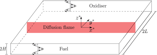
Figure 1. Schematic diagram of a planar diffusion flame aligned parallel to a shear flow in a narrow channel ($H\ll L$). The fuel and oxidizer reach the flame by diffusion from opposite sides.

The appeal to Taylor dispersion as a mechanism in explaining the formation of flame streets has been validated by Rajamanickam, Kelly, and Daou (2023) within an idealized constant-density adiabatic model adopting the configuration of Figure 1. The neglect of heat loss in this model was intended to demonstrate that Taylor dispersion can induce, on its own, a cellular instability for large $Le$ which is able to explain the experimental observations on flame streets. However, since heat losses are expectedly significant (Mohan and Matalon 2017) in micro-combustion experiments, it is important to assess their influence on the findings reported by Rajamanickam, Kelly, and Daou (2023). This is the main objective of the current investigation, which focuses on examining the diffusive-thermal instability of planar diffusion flames aligned with the shear flow direction, specifically under the combined influence of heat losses and Taylor dispersion. It is worth noting that such investigations have been reported using the same model configuration considered here, but in the absence of Taylor dispersion (Miklavčič, Moore, and Wichman 2005; Sohn et al. 2000).

The paper is organized as follows. The two-dimensional depth-averaged governing equations, derived in the limit $H\ll L$, are presented in $\mathcal{\S }$2 and clearly feature the presence of anisotropic diffusion. Based on these equations, an eigen-boundary-value problem is derived in $\mathcal{\S }$3 to study the linear stability of the planar diffusion flame sketched in Figure 1. The results of the linear stability analysis, based on the computation of eigenvalues, are presented in $\mathcal{\S }$4 where three types of instability are identified and located in stability regime diagrams in the $Le$-$Pe$ plane. Time-dependent numerical solutions are presented in $\mathcal{\S }$5 for selected cases, confirming the occurrence of the flame instabilities and illustrating the non-linear evolution of unstable flames.

Formulation

Consider the narrow channel geometry shown in Figure 1 which is infinitely long in the $x^{\ast }$-direction. The channel height $2H$ and the width $2L$ are assumed to satisfy the condition $H\ll L$. The fluid motion in the channel is assumed for simplicity to correspond to a fully developed Poiseuille flow along the $x^{\ast }$-direction, and the frame of reference is chosen to be moving with the mean flow velocity $U$ so that the velocity components can be written as

(1) $v_x^{\ast }=\frac{U}{2}\left(1-\frac{3z^{\ast 2}}{H^2}\right),v_y^{\ast }=v_z^{\ast }=0.$(1)

Alternatively, one can adopt a zero-mean Couette flow which would be also suitable for our main purpose, namely identifying the coupling between shear-enhanced diffusion and the instability of the non-adiabatic flame.

As done by Rajamanickam, Kelly, and Daou (2023), we shall assume that the mass fractions of the fuel $Y_F^{\ast }$ and the oxidizer $Y_O^{\ast }$ are maintained fixed at $y^{\ast }=\pm L$, with $Y_F^{\ast }=Y_{F,F}^{\ast }$, $Y_O^{\ast }=0$ on the fuel side ($y^{\ast }=-L$) and $Y_O^{\ast }=Y_{O,O}^{\ast }$, $Y_F^{\ast }=0$ on the oxidizer side ($y^{\ast }=+L$). A planar diffusion flame is shown in the middle of the channel which is maintained by diffusion of the reactants along the $y^{\ast }$-direction. To model the conductive heat losses to the channel walls in a simple way, we adopt the boundary condition

(2) $\frac{\mathrm{\partial }{T}^{\ast }}{\mathrm{\partial }{z}^{\ast }}=-K(T^{\ast }-T_u^{\ast }),\mathrm{a}\mathrm{t}{z}^{\ast }=\pm H,$(2)

where $K$ is a heat transfer coefficient, $T^{\ast }$ the temperature and $T_u^{\ast }$ the temperature in the oxidizer and fuel sides at $y^{\ast }=\pm L$. We note that the model may be extended to include radiative losses to the walls and possibly also reabsorption effects in the gas phase as done by Smooke et al. (2005), Zheng et al. (2022).

The chemistry is modeled by the one-step irreversible Arrhenius reaction

$\mathrm{F}\mathrm{u}\mathrm{e}\mathrm{l}+s{\mathrm{O}}_2->\mathrm{P}\mathrm{r}\mathrm{o}\mathrm{d}\mathrm{u}\mathrm{c}\mathrm{t}\mathrm{s}+q$

where $q$ and $s$ denote the amount of energy released and mass of oxidizer consumed per unit mass of fuel burnt. The rate of fuel mass burnt per unit volume is assumed to be equal to ${\rho }^{2}B{Y}_F^{\ast }{Y}_O^{\ast }exp(-E/R{T}^{\ast })$, where $B$ is a pre-exponential factor, $\rho$ is the density of the mixture (assumed to be constant), $E$ is the activation energy and $R$ is the universal gas constant. The heat release parameter $\alpha$, the Zeldovich number $\beta$, the Damköhler number $Da$ and the stoichiometry parameter $S$ are defined by

(3) $\alpha =\frac{T_{ad}^{\ast }-T_u^{\ast }}{T_{ad}^{\ast }},\beta =\frac{\alpha E}{R{T}_{ad}^{\ast }},Da=\frac{L^2/D_T}{{\beta }^3{[B\rho Y_{O,O}^{\ast }exp(-E/R{T}_{ad}^{\ast })]}^{-1}},S=\frac{s{Y}_{F,F}^{\ast }}{Y_{O,O}^{\ast }},$(3)

where $T_{ad}^{\ast }=T_u^{\ast }+q{Y}_{F,F}^{\ast }/c_p(S+1)$ is the adiabatic flame temperature at the stoichiometric location, $D_T$ is the thermal diffusivity and $c_p$ is the constant-pressure specific heat. In this paper, we will assume that the diffusivity of the oxidizer is equal to the thermal diffusivity, and therefore the oxidizer Lewis number $Le{}_O=1$. The fuel Lewis number $Le{}_F$ will be simply denoted by $Le$.

To facilitate the analysis, we introduce the nondimensional and scaled variables

(4) $t=\frac{t^{\ast }}{L^2/D_T},(x,y,z)=\frac{1}{L}(x^{\ast },y^{\ast },z^{\ast }/ϵ),Y_F=\frac{Y_F^{\ast }}{Y_{F,F}^{\ast }},Y_O=\frac{Y_O^{\ast }}{Y_{O,O}^{\ast }},\theta =\frac{T^{\ast }-T_u^{\ast }}{T_{ad}^{\ast }-T_u^{\ast }},$(4)

where the parameter $ϵ=H/L$ will be regarded as being small. The resulting governing equations, in the thermo-diffusive approximation, reduce to

(5) $\frac{\mathrm{\partial }{Y}_F}{\mathrm{\partial }t}+\frac{Pe}{2ϵ}(1-3z^2)\frac{\mathrm{\partial }{Y}_F}{\mathrm{\partial }x}=\frac{1}{Le}\left(\frac{{\mathrm{\partial }}^2{Y}_F}{\mathrm{\partial }{x}^2}+\frac{{\mathrm{\partial }}^2{Y}_F}{\mathrm{\partial }{y}^2}+\frac{1}{{ϵ}^2}\frac{{\mathrm{\partial }}^2{Y}_F}{\mathrm{\partial }{z}^2}\right)-Da\omega ,$(5)

(6) $\frac{\mathrm{\partial }{Y}_O}{\mathrm{\partial }t}+\frac{Pe}{2ϵ}(1-3z^2)\frac{\mathrm{\partial }{Y}_O}{\mathrm{\partial }x}=\frac{{\mathrm{\partial }}^2{Y}_O}{\mathrm{\partial }{x}^2}+\frac{{\mathrm{\partial }}^2{Y}_O}{\mathrm{\partial }{y}^2}+\frac{1}{{ϵ}^2}\frac{{\mathrm{\partial }}^2{Y}_O}{\mathrm{\partial }{z}^2}-SDa\omega ,$(6)

(7) $\frac{\mathrm{\partial }\theta }{\mathrm{\partial }t}+\frac{Pe}{2ϵ}(1-3z^2)\frac{\mathrm{\partial }\theta }{\mathrm{\partial }x}=\frac{{\mathrm{\partial }}^2\theta }{\mathrm{\partial }{x}^2}+\frac{{\mathrm{\partial }}^2\theta }{\mathrm{\partial }{y}^2}+\frac{1}{{ϵ}^2}\frac{{\mathrm{\partial }}^2\theta }{\mathrm{\partial }{z}^2}+(S+1)Da\omega ,$(7)

where we have introduced the Péclet number $Pe=UH/D_T$ and the normalized reaction rate

(8) $\omega ={\beta }^3{Y}_F{Y}_{O}exp\left[\frac{\beta (\theta -1)}{1+\alpha (\theta -1)}\right].$(8)

Assuming symmetry about the $xy$-plane, the boundary conditions in the $z$-direction can be written as

(9) $\frac{\mathrm{\partial }{Y}_F}{\mathrm{\partial }z}=\frac{\mathrm{\partial }{Y}_O}{\mathrm{\partial }z}=\frac{\mathrm{\partial }\theta }{\mathrm{\partial }z}=0,\mathrm{a}\mathrm{t}z=0,$(9)

(10) $\frac{\mathrm{\partial }{Y}_F}{\mathrm{\partial }z}=\frac{\mathrm{\partial }{Y}_O}{\mathrm{\partial }z}=\frac{\mathrm{\partial }\theta }{\mathrm{\partial }z}+{ϵ}^2\kappa Da\theta =0,\mathrm{a}\mathrm{t}z=1,$(10)

where the nondimensional heat-loss parameter $\kappa$ is defined as

(11) $\kappa =\frac{LK}{ϵDa}.$(11)

The heat loss parameter $\kappa$ represents the ratio of a characteristic heat-loss rate $\rho c_{p}K(T_{ad}^{\ast }-T_u^{\ast })$ to a characteristic heat-release rate $\rho c_p(T_{ad}^{\ast }-T_u^{\ast })HDa/(L^2/D_T)$ per unit cross-section of the channel wall.

In the limit $ϵ\to 0$, all dependent variables become uniform in the $z$-direction in the first approximation and the convective terms on the left-hand side of (5)-(7) manifest upon depth-averaging as the enhanced diffusion terms in the $x^{\ast }$-direction as done by Daou (2021), Daou and Rajamanickam (2023, 2018), Daou and Rajamanickam (2023), Liñán et al. (2020), Pearce and Daou (2014), Rajamanickam and Daou (2023), Rajamanickam, Kelly, and Daou (2023), Rajamanickam and Weiss (2022). We thus obtain the two-dimensional governing equations

(12) $\frac{\mathrm{\partial }{Y}_F}{\mathrm{\partial }t}=\frac{1}{Le}\left[(1+p^{2}Le{}^2)\frac{{\mathrm{\partial }}^2{Y}_F}{\mathrm{\partial }{x}^2}+\frac{{\mathrm{\partial }}^2{Y}_F}{\mathrm{\partial }{y}^2}\right]-Da\omega ,$(12)

(13) $\frac{\mathrm{\partial }{Y}_O}{\mathrm{\partial }t}=(1+p^2)\frac{{\mathrm{\partial }}^2{Y}_O}{\mathrm{\partial }{x}^2}+\frac{{\mathrm{\partial }}^2{Y}_O}{\mathrm{\partial }{y}^2}-SDa\omega ,$(13)

(14) $\frac{\mathrm{\partial }\theta }{\mathrm{\partial }t}=(1+p^2)\frac{{\mathrm{\partial }}^2\theta }{\mathrm{\partial }{x}^2}+\frac{{\mathrm{\partial }}^2\theta }{\mathrm{\partial }{y}^2}+Da\left[(S+1)\omega -\kappa \theta \right],$(14)

where $p=\sqrt{\gamma }Pe$ is a scaled Péclet number and $\gamma =2/105$ for the plane Poiseuille flow adopted. Note that the equations clearly exhibit anisotropic diffusion, involving the effective flow-dependent Lewis number $Le(1+p^2)/(1+p^{2}Le{}^2)$ in the $x$-direction and the ordinary Lewis number $Le$ in the $y$-direction. Note also that in the narrow channel limit considered, the conductive heat losses at the channel walls appear now as a volumetric heat loss in the energy equation as in Daou and Matalon (2002), Rajamanickam and Daou (2023).

The equations above are subject to the boundary conditions

(15) $Y_F=1,Y_O=0,\theta =0,\mathrm{a}\mathrm{t}y=-1,$(15)

(16) $Y_F=0,Y_O=1,\theta =0,\mathrm{a}\mathrm{t}y=+1.$(16)

In the $x$-direction, periodic boundary conditions are adopted for the sake of simplicity and in order to avoid complications related to entrance and exit conditions. The reader is directed to Kang et al. (2019), Mackay, Johnson, and Freund (2019), Mohan and Matalon (2017) for studies accounting for such conditions.

Linear stability analysis

Unperturbed planar diffusion flames

In this subsection, we describe the steady, planar diffusion flame solutions, whose stability will be addressed in the following subsection. These solutions are governed by

(17) $\frac{1}{Le}\frac{d^2{\bar{Y}}_F}{d{y}^2}=\frac{1}{S}\frac{d^2{\bar{Y}}_O}{d{y}^2}=\frac{1}{S+1}\left(\kappa Da\bar{\theta }-\frac{d^2\bar{\theta }}{d{y}^2}\right)=Da\omega ,$(17)

obtained by setting $\mathrm{\partial }/\mathrm{\partial }x=\mathrm{\partial }/\mathrm{\partial }t=0$ in (12)-(14). Here, the overbar refers to the unperturbed state. Integrating the first equation, we obtain

(18) ${\bar{Y}}_O=\frac{S}{Le}\left[{\bar{Y}}_F+\frac{1}{2}(y-1)\right]+\frac{1}{2}(y+1),$(18)

which allows the function $\omega ({\bar{Y}}_F,{\bar{Y}}_O,\bar{\theta })$ to be written as $\omega ({\bar{Y}}_F,\bar{\theta },y)$. This results in the equations

(19) $\frac{1}{Le}\frac{d^2{\bar{Y}}_F}{d{y}^2}=\frac{1}{S+1}\left(\kappa Da\bar{\theta }-\frac{d^2\bar{\theta }}{d{y}^2}\right)=Da\omega ({\bar{Y}}_F,\bar{\theta },y)$(19)

which will be solved numerically, subject to the boundary conditions

(20) ${\bar{Y}}_F=1,\bar{\theta }=0,\mathrm{a}\mathrm{t}y=-1,$(20)

(21) ${\bar{Y}}_F=0,\bar{\theta }=0,\mathrm{a}\mathrm{t}y=+1.$(21)

The numerical solutions are determined using COMSOL Multiphysics software as done by Rajamanickam, Kelly, and Daou (2023). The computations are performed for a wide range of values of $Da$, $Le$ and $\kappa$ and for the fixed values $\alpha =0.85$, $\beta =10$ and $S=1$ with the last condition characterizing a stoichiometric mixture. The results are summarized in the next two figures.

Figure 2 determines the existence domain of the planar flame solutions in $Le$-$\kappa$ plane. These (burning) solutions are found to exist only if the heat-loss parameter $\kappa$ is less than a critical quenching value ${\kappa }_q$ plotted in the figure, which is independent of $Da$. The nearly linear behavior of the log plot indicates that ${\kappa }_q$ decreases exponentially as $Le$ increases. Using ${\kappa }_q$, we introduce the ratio

Figure 2. Critical quenching value ${\kappa }_q$ versus the Lewis number $Le$. Planar flame solutions (which are not nearly frozen) exist only below the plotted line.

(22) ${\kappa }_{\ast }=\frac{\kappa }{{\kappa }_q}$(22)

which allows the existence domain of the planar diffusion flames to be characterized by ${\kappa }_{\ast }<1$, irrespective of the value of $Le$. Note that for $0\le {\kappa }_{\ast }<1$, Equations (19)(19) $\frac{1}{Le}\frac{d^2{\bar{Y}}_F}{d{y}^2}=\frac{1}{S+1}\left(\kappa Da\bar{\theta }-\frac{d^2\bar{\theta }}{d{y}^2}\right)=Da\omega ({\bar{Y}}_F,\bar{\theta },y)$(19) admit typically either one or three solutions for a given $Da$, including a nearly frozen solution, whereas for ${\kappa }_{\ast }>1$, only a nearly frozen solution exists. We shall use ${\kappa }_{\ast }$ instead of $\kappa$ below as it is more convenient when comparing cases with different Lewis numbers, such as for the two cases in Figure 3.

Figure 3. Maximum temperature ${\bar{\theta }}_{\mathrm{m}\mathrm{a}\mathrm{x}}$ versus $Da$ for $Le=0.5$ on the left and $Le=2$ on the right, for selected values of ${\kappa }_{\ast }$. For any ${\kappa }_{\ast }\ne 0$, the left turning point (blue asterisk) corresponds to diffusive extinction occurring at $Da=Da{}_d$ and the right turning point (red asterisk) to heat-loss extinction occurring at $Da=Da{}_{hl}$.

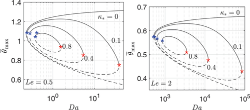
Shown in this figure is maximum temperature ${\bar{\theta }}_{\mathrm{m}\mathrm{a}\mathrm{x}}=\mathrm{m}\mathrm{a}\mathrm{x}(\bar{\theta })$ as a function of $Da$ for $Le=0.5$ (left subfigure) and $Le=2$ (right subfigure). In the absence of heat loss (${\kappa }_{\ast }=0$), one recovers the familiar S-shaped ignition-extinction curve (Liñán 1974), consisting of an upper strongly burning, near-equilibrium branch (solid lines), an intermediate partial burning branch (dashed lines) and a lower, nearly frozen branch (not shown). In the presence of heat-loss, ${\kappa }_{\ast }>0$,¹, one obtains, however, a closed loop delimiting an island in the $Da$-${\bar{\theta }}_{\mathrm{m}\mathrm{a}\mathrm{x}}$ plane. For each value of ${\kappa }_{\ast }$, the corresponding closed loop possesses two extinction (turning) points where the solid and dashed lines meet. The left turning point will be referred to as the diffusive extinction point (Williams 2000) and this corresponds to $Da=Da{}_d$, say. As for the right turning point, which only exists when ${\kappa }^{\ast }>0$, it will be referred to as the heat-loss extinction point (Williams 2000) and this corresponds to $Da=Da{}_{hl}$, say. As ${\kappa }_{\ast }$ is varied, $Da{}_d$ varies mildly in comparison with $Da{}_{hl}$ which undergoes drastic change. As ${\kappa }_{\ast }\to 1$, the two extinction Damköhler numbers approach each other, leading to the disappearance of the loop for ${\kappa }_{\ast }>1$.

To close this subsection, we note parenthetically that it is possible to describe the planar flame solutions using perturbation methods in the distinguished asymptotic limit $\hat{\beta }\to \mathrm{\infty }$ with $\kappa Da$ being finite (Chao, Law, and T’ien 1991; Sohn et al. 2000); here $\hat{\beta }$ denotes the Zeldovich number based on the non-adiabatic reaction-sheet temperature. For example, the strongly burning solutions appearing as solid lines in Figure 3 can be described (away from the turning points) by the leading-order approximation obtained in Appendix A. This asymptotic approach will not be pursued any further as we turn now to a numerical linear stability analysis.

Formulation of the linear stability problem

In this paper, we shall focus only on the stability of the strongly-burning near-equilibrium solutions, corresponding to the solid lines in Figure 3 and ignore other branches. To this end, we introduce small-amplitude perturbations of the form

(23) $\left[\begin{array}{c}{Y}_F\\ Y_O\\ \theta \end{array}\right]=\left[\begin{array}{c}{\bar{Y}}_F(y)\\ {\bar{Y}}_O(y)\\ \bar{\theta }(y)\end{array}\right]+\left[\begin{array}{c}{\tilde{Y}}_F(y)\\ {\tilde{Y}}_O(y)\\ \tilde{\theta }(y)\end{array}\right]e^{ikx+\sigma t}$(23)

where we have denoted the perturbed variables with a tilde symbol. Here $k$ represents the real wavenumber of the perturbation and $\sigma$ is the growth rate (in general, complex), which is to be obtained as an eigenvalue.

Substituting (23) into the governing equations (12)-(14) and linearizing, we obtain the eigenvalue problem

(24) $\sigma {\tilde{Y}}_F=\frac{k^2}{Le}(1+p^{2}Le{}^2){\tilde{Y}}_F+\frac{1}{Le}\frac{d^2{\tilde{Y}}_F}{d{y}^2}-Da\tilde{\omega },$(24)

(25) $\sigma {\tilde{Y}}_O=-k^2(1+p^2){\tilde{Y}}_O+\frac{d^2{\tilde{Y}}_O}{d{y}^2}-SDa\tilde{\omega },$(25)

(26) $\sigma \tilde{\theta }=-k^2(1+p^2)\tilde{\theta }+\frac{d^2\tilde{\theta }}{d{y}^2}+Da\left[(S+1)\tilde{\omega }-\kappa \tilde{\theta }\right],$(26)

where

(27) $\tilde{\omega }={\beta }^3\left\{{\tilde{Y}}_F{\bar{Y}}_O+{\tilde{Y}}_O{\bar{Y}}_F+\frac{\beta {\bar{Y}}_F{\bar{Y}}_O\tilde{\theta }}{{[1+\alpha (\bar{\theta }-1)]}^2}\right\}exp\left[\frac{\beta (\bar{\theta }-1)}{1+\alpha (\bar{\theta }-1)}\right].$(27)

The eigenvalue problem is to be solved numerically subject to homogeneous Dirichlet boundary conditions at $y=\pm 1$. The problem possesses a discrete spectrum of eigenvalues ${\sigma }_n$ indexed by an integer $n$, which are computed using the Chebfun package (Driscoll, Hale, and Trefethen 2014), a package based on a spectral collocation method using Chebyshev polynomials.

Flame stability results and bifurcation diagrams

Preliminary remarks and terminology

The eigenvalue with the largest real part (largest real growth rate) among the eigenvalues ${\sigma }_n$ determines the stability of the planar solution for a given set of parameters. Henceforth, $\sigma$ will always denote this particular leading eigenvalue which depends on the parameters in the form

$\sigma =\sigma (k;Le,p,Da,\kappa )$

for fixed values of $\beta$, $\alpha$ and $S$.

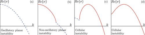
The function $\sigma (k)$ is computed numerically by varying the parameters $Le$, $p$, $Da$ and $\kappa$. Its curves take, in general, one of the four types schematically shown in Figure 4. We have labeled these four types based on whether the most unstable mode, corresponding to the maximum of $\mathrm{R}\mathrm{e}(\sigma )$ is oscillatory or not and whether it occurs at $k=0$ or not. Thus, an oscillatory planar instability corresponds to cases where the most unstable mode occurs at $k=0$ with growth rate $\sigma$ having a non-zero imaginary part. Similarly, a non-oscillatory planar instability corresponds to cases where the most unstable mode occurs at $k=0$ with growth rate $\sigma$ having a zero imaginary part. Finally, a cellular instability represents cases where the most unstable mode lies at $k\ne 0$ with $\sigma$ being real valued.

Figure 4. Schematic diagram illustrating the types of instability depending on the function $\sigma (k)$ whose real part is plotted versus $k$. Solid lines represent real branches ($\mathrm{I}\mathrm{m}\{\sigma \}=0$) and dashed lines complex branches ($\mathrm{I}\mathrm{m}\{\sigma \}\ne 0$).

The diffusive-thermal flame instability typically occurs in near-extinction conditions, that is for $Da$ being either close to the diffusive-extinction Damköhler number $Da{}_d$ or to the heat-loss extinction Damköhler number $Da{}_{hl}$. Therefore, we shall focus on examining the flame instability near these two extinction points. To this end, it is convenient to introduce the parameters

(28) $\delta =\frac{Da-Da{}_d}{Da{}_d},\mathrm{\Delta }=\frac{Da{}_{hl}-Da}{Da{}_{hl}},$(28)

which measure the relative departure of the Damköhler number from these extinction values. Associated with these parameters are critical values ${\delta }_c={\delta }_c(Le,p)$ and ${\mathrm{\Delta }}_c={\mathrm{\Delta }}_c(Le,p)$ such that the planar diffusion flame is expected to be unstable for $0\le \delta \le {\delta }_c$ and $0\le \mathrm{\Delta }\le {\mathrm{\Delta }}_c$. For $Da$ between the Damköhler numbers corresponding to ${\delta }_c$ and ${\mathrm{\Delta }}_c$, namely for $Da\in [Da{}_d(1+{\delta }_c),Da{}_{hl}(1-{\mathrm{\Delta }}_c)]$, the flame is found to be stable provided ${\kappa }_{\ast }$ is not too close to unity. For example, when $Le=2$, a portion of the upper branch in Figure 3 is still stable when ${\kappa }_{\ast }=0.9$, but the whole branch becomes unstable when ${\kappa }_{\ast }>0.933$.

Before presenting the numerical results, it is worth pointing out that the diffusive-thermal instability of the planar diffusion flame in our configuration has been investigated by Miklavčič, Moore, and Wichman (2005), Sohn et al. (2000). These studies do not address, however, the effect of shear-enhanced diffusion present in our depth-averaged equations and correspond therefore to the $p=0$ case. Furthermore, they are based on a radiative rather than a conductive heat-loss model adopted herein. In these studies, only planar instabilities have been found, while no cellular instabilities, such as the one to be identified below, have been encountered. These planar instabilities have been shown to exist only in $Le>1$ mixtures for adiabatic flames (Sohn, Chung, and Kim 1999; Vance, Miklavčič, and Wichman 2001) but can also exist in $Le<1$ mixtures in the presence of heat losses. In the next two subsections, we shall examine how accounting for Taylor dispersion can modify such predictions when $p\ne 0$.

Influence of heat loss on flame instability near diffusive-extinction conditions

In this subsection, we examine the stability of the strongly-burning planar solutions in the neighborhood of the diffusive extinction points, the left turning points in Figure 3.

We begin by revisiting the adiabatic case, ${\kappa }_{\ast }=0$, which was analyzed by Rajamanickam, Kelly, and Daou (2023). The analysis produces a stability regime diagram in the $Le$-$p$ plane such as that shown in the left subfigure of Figure 5, for $\delta =0.01$. The diagram determines the type of instabilities and shows that these occur only in $Le>1$ mixtures. More importantly, it also indicates that cellular instability surprisingly emerges in such $Le>1$ mixtures, provided $p$ exceeds a critical value. Below this critical value, we encounter planar instabilities, either of oscillatory or non-oscillatory type depending on the values of $Le$. As the parameters $p$ and $Le$ are varied from values taken in the purple region (oscillatory planar instability) to values taken in the green region (cellular instability), a jump transition takes place corresponding to a transition of the dispersion curve from the type shown in Figure 4(a) to that in Figure 4(c). Similarly, the transition from non-oscillatory planar (red region) to cellular (green region) instability corresponds to a continuous transition of the dispersion curve from Figures 4(b-d).

Figure 5. Stability regime diagrams in the $Le$-$p$ plane for three values of ${\kappa }_{\ast }$, identifying the regions of the planar flame instability types near the diffusive extinction point. OPI is an abbreviation for oscillatory planar instability and NOPI is an abbreviation for non-oscillatory planar instability.

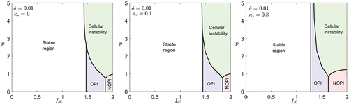
We can now examine the influence of heat loss on the stability results by reproducing the similar stability diagrams, as done in middle and the right subfigures of Figure 5 for two selected values of ${\kappa }_{\ast }$. The diagrams indicate that instability regions identified in the adiabatic case persist in the nonadiabatic cases, although the boundaries of their existence domains are shifted to lower Lewis numbers. This shift is seen to be more pronounced for larger values of ${\kappa }_{\ast }$. Furthermore, as ${\kappa }_{\ast }$ is increased, the boundary between the stable region and the oscillatory instability region extends to a wider range of $p$. Meanwhile, the boundary between the stable region and the cellular instability region shrinks and disappears for sufficiently large values of ${\kappa }_{\ast }$. For such large values, as in the case of the right subfigure, the boundary between the stable region and the oscillatory instability region is found to extend vertically to $p\to \mathrm{\infty }$. Note that in this case, a direct transition from stable to cellular flames is no more possible, unlike for the cases of the other two subfigures. In general, the diagrams demonstrate that heat loss promotes all types of instabilities identified in the adiabatic case, but to a greater extent for the planar instabilities. It is also worth mentioning based on our computations that flame instabilities in near diffusive-extinction conditions are found to occur only in $Le>1$ mixtures, even in the presence of heat losses.

Flame instability near heat-loss extinction conditions

In this subsection, we examine the stability of the strongly-burning planar solutions in the neighborhood of the heat-loss extinction points, the right turning points in Figure 3.

To this end, three values of ${\kappa }_{\ast }$ are considered and corresponding stability diagrams, similar to those of Figure 5, are presented in Figure 6. The diagrams pertain to $\mathrm{\Delta }=0.01$ and selected values of ${\kappa }_{\ast }$ increasing from left to right. Several remarks can be made with respect to these diagrams:

Figure 6. Stability regime diagrams in the $Le$-$p$ plane for three values of ${\kappa }_{\ast }$, identifying the regions of the planar flame instability types near the heat-loss extinction point. OPI is an abbreviation for oscillatory planar instability and NOPI is an abbreviation for non-oscillatory planar instability.

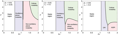
1. First of all, we note that all three types of instabilities identified in Figure 5 are also present in Figure 6.

2. Comparing the right subfigure in Figure 6 with the right subfigure of Figure 5, both corresponding to ${\kappa }_{\ast }=0.8$, we note that instability domains have similar structure.

3. As ${\kappa }_{\ast }$ is decreased, the boundaries between different regions in the subfigures of Figure 6 shift to the left toward smaller values of $Le$, a fact which is consistent with the $p=0$ results presented in Figure 7 of the paper by Sohn et al. (2000). This behavior is in contrast to that observed in Figure 5.

4. Further, the shift to the left as ${\kappa }_{\ast }$ is decreased in Figure 6 indicates that $Le\le 1$ mixtures can exhibit instability of the oscillatory planar type only. In particular, cellular and non-oscillatory planar type instabilities are not found in $Le\le 1$ mixtures.

5. In addition, the shift to the left mentioned above is accompanied by the peak of the boundary between the non-oscillatory and cellular instability region moving upwards and pushed to infinity for sufficiently small values of ${\kappa }_{\ast }$, as in the case of the left subfigure.

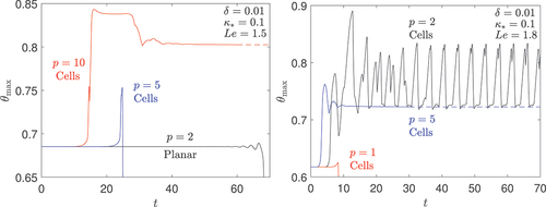
Figure 7. Maximum temperature ${\theta }_{\mathrm{m}\mathrm{a}\mathrm{x}}$ over the domain as a function of time $t$ for $Le=1.5$ (left) and $Le=1.8$ (right) and for selected values of $p$. The label “cells” characterises cases where cells are observed in the simulations at the onset of instability; see illustrative two-dimensional figures below. The label “planar” characterises cases where the unstable flame is observed to remain planar.

To close this subsection, we note that out of the three instability types identified, two are already present in the absence of Taylor dispersion, that is when $p=0$, which is consistent with the findings in the literature (Miklavčič, Moore, and Wichman 2005; Sohn et al. 2000). The presence of Taylor dispersion creates an additional type of instability, namely the cellular instability type, provided $Le>1$ and $p$ is above a critical value.

Time-dependent numerical simulations

The stability analysis, based on the computations of the eigenvalues of the linear stability problem, has identified the types of instability encountered and their existence domains in terms of the parameters $Le$, $p$, $Da$ and ${\kappa }_{\ast }$. To confirm the existence of these instabilities and illustrate their development, we present in this section time-dependent numerical solutions of Equations (12)(12) $\frac{\mathrm{\partial }{Y}_F}{\mathrm{\partial }t}=\frac{1}{Le}\left[(1+p^{2}Le{}^2)\frac{{\mathrm{\partial }}^2{Y}_F}{\mathrm{\partial }{x}^2}+\frac{{\mathrm{\partial }}^2{Y}_F}{\mathrm{\partial }{y}^2}\right]-Da\omega ,$(12) - (14(14) $\frac{\mathrm{\partial }\theta }{\mathrm{\partial }t}=(1+p^2)\frac{{\mathrm{\partial }}^2\theta }{\mathrm{\partial }{x}^2}+\frac{{\mathrm{\partial }}^2\theta }{\mathrm{\partial }{y}^2}+Da\left[(S+1)\omega -\kappa \theta \right],$(14) ). These are subject to the Dirichlet conditions (15)-(16) at $y=\pm 1$, along with periodic boundary conditions in the $x$-direction. The initial condition for the computations corresponds to the steady planar diffusion flame, discussed in $\mathcal{\S }$3.1. We note that the periodicity conditions in the $x$-direction are suitable for our idealized simple model and allow in particular to avoid complicating extraneous effects associated with special inlet/outlet conditions encountered in experiments.

The computations are carried out using the COMSOL multiphysics software, as has been done previously (Daou 2021, Daou et al., 2023; Rajamanickam, Kelly, and Daou 2023). The domain size is chosen to be $x\in [-15\sqrt{1+p^2},15\sqrt{1+p^2}]$ and $y\in [-1,1]$, which allows to capture sufficient number of cells in the case of cellular instability. The results to be presented correspond to cases with $\alpha =0.85$, $\beta =10$, $S=1$, $\delta =\mathrm{\Delta }=0.01$ and selected values of $p$, $Le$ and ${\kappa }_{\ast }$.

Numerical results for near diffusive-extinction conditions

In this subsection, we present numerical results illustrating the instabilities, identified in Figure 5, of strongly-burning planar flame solutions in the neighborhood of the diffusive extinction points (the left turning points in Figure 3). The simulations correspond to nonadiabatic cases with ${\kappa }_{\ast }=0.1$ pertaining to the middle stability diagram in Figure 5. Adiabatic cases with ${\kappa }_{\ast }=0$ pertaining to the left stability diagram in Figure 5 can be found in the paper by Rajamanickam, Kelly, and Daou (2023).

We begin by discussing Figure 7 where results corresponding to three cases with $Le=1.5$ and selected values of $p$ are presented in the left subfigure and three cases with $Le=1.8$ and selected values of $p$ in the right subfigure. Shown is the maximum temperature ${\theta }_{\mathrm{m}\mathrm{a}\mathrm{x}}$ plotted against time $t$. The selected cases all pertain to points in the unstable regions in the middle subfigure of Figure 5 and the figure confirms indeed the flame instability, as ${\theta }_{\mathrm{m}\mathrm{a}\mathrm{x}}$ does not remain equal to its initial value. In the figure, we have added the label “Cells” for the cases where a cellular pattern is observed in the simulations at the onset of instability. Similarly, we have added the label “Planar” to cases where the unstable flame is observed to remain planar.

For example, when $p=2$, an oscillatory planar instability is obtained with ${\theta }_{\mathrm{m}\mathrm{a}\mathrm{x}}$ exhibiting amplified oscillations in time which ultimately lead to total extinction. On the other hand, for the cases with $p=5$ and $p=10$, cells are observed near the instability onset, in the form of alternating flame segments with strong and weak reaction rates. Ultimately, these cells can experience total quenching as in the $p=5$ case, or can lead to an apparently stable cellular pattern as in the $p=10$ case. This stable pattern is seen in the top subfigure of Figure 8 where the reaction-rate $\omega$-field is shown at $t=60$. Similar cellular instability is observed for the $Le=1.8$ cases considered in the right subfigure of Figure 7. This leads ultimately to a quenched state as for $p=1$ or to an apparently stable steady cellular pattern as for $p=5$, this pattern being shown in the bottom subfigure of Figure 7. The unstable flame can also experience more complex dynamics involving triple-flame propagation, splitting and merging of cells, etc., as in the case of $p=2$, whose dynamics is shown in Figure 9. The complex dynamics can, however, be better appreciated from the animated time evolution which is included as a supplementary material.

Figure 8. Reaction rate $\omega$-fields showing stable cellular structures at large times ($t=60$ for the top subfigure and $t=30$ for the bottom subfigure).

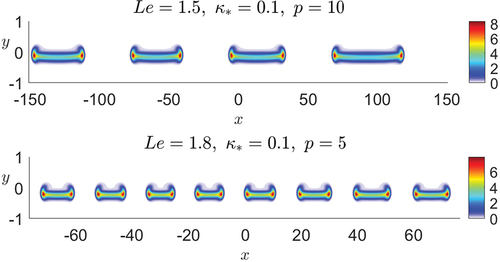
Figure 9. Reaction rate $\omega$-fields at selected values of time, illustrating the flame evolution near the diffusive extinction point.

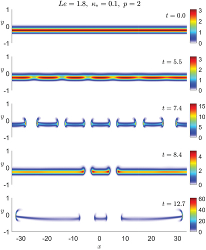
It is worth pointing out that the dynamic scenarios described are also found for adiabatic flames (Rajamanickam, Kelly, and Daou 2023), except the one where the cellular instability leading to total extinction. Overall, the results suggest that the cells formed, following a Taylor dispersion-induced cellular instability, require higher values of $p$ and $Le$ to be stabilized, in order to counteract quenching by heat losses.

Numerical results for near heat loss-extinction conditions

In this subsection, we present numerical results illustrating the instabilities, identified in Figure 6, of strongly-burning planar flame solutions in the neighborhood of the heat-loss extinction points (the right turning points in Figure 3). The simulations correspond to cases with ${\kappa }_{\ast }=0.05$ and ${\kappa }_{\ast }=0.1$ pertaining to the left and the middle stability diagrams in Figure 6.

Shown in Figure 10 is the maximum temperature ${\theta }_{\mathrm{m}\mathrm{a}\mathrm{x}}$ plotted against time $t$. The cases selected in the left subfigure illustrate the occurrence of the oscillatory planar instability, particularly for values of $Le\le 1$, leading ultimately to total extinction. It is worth emphasizing that such oscillations for $Le\le 1$ do not occur in near diffusive-extinction conditions, as mentioned in $\mathcal{\S }$4.3, but they are known to occur in near heat-loss extinction conditions, as noted in earlier works (Cheatham and Matalon 1996; Kukuck and Matalon 2001; Sohn et al. 2000).

Figure 10. Maximum temperature ${\theta }_{\mathrm{m}\mathrm{a}\mathrm{x}}$ over the domain as a function of time $t$. The cases in the left subfigure are selected to illustrate the oscillatory planar instability. Those in the right subfigure are selected to illustrate the cellular instability.

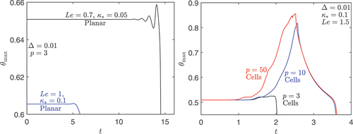
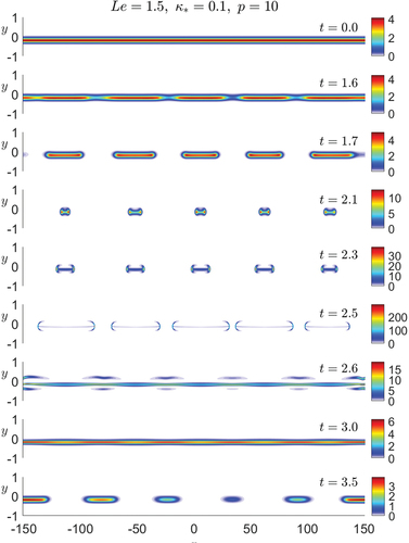
As for the cases in the right subfigure of Figure 10, they are selected to illustrate the occurrence of the cellular instability for $Le=1.5$. For this particular value of $Le$, the cellular structure emerging at the instability onset undergoes complex dynamics leading ultimately to total extinction, irrespective of the value of $p$. An illustration of this evolution is shown in Figure 11 for $p=10$ and is included in the form of an animation as a supplementary material. Note, however, that the Taylor dispersion-induced cellular instability can also lead ultimately to a stable cellular structure, for example, for $Le=2$ and $p\sim 1$ as found in our computations (not shown here).

Figure 11. Reaction rate $\omega$-fields at selected values of time, illustrating the flame evolution near the heat-loss extinction point.

Conclusions

We have investigated the diffusive-thermal stability of a planar diffusion flame aligned with the direction of a shear flow in a narrow channel, accounting for conductive heat losses to surrounding walls. The study is based on a simple model derived for narrow channels, which incorporates Taylor dispersion, or shear-enhanced diffusion, as well as heat losses. The investigation relies on a linear stability analysis, based on the computation of eigenvalues, and on time-dependent numerical simulations. The work extends a previous investigation (Rajamanickam, Kelly, and Daou 2023) ignoring heat losses, which has unveiled a new cellular instability, induced by Taylor dispersion, occurring in $Le>1$ mixtures. Since heat losses are expectedly important in micro-combustion devices, it is imperative to examine how they affect the Taylor dispersion-induced cellular instability, which is the main concern of this paper.

The study has focused on near extinction conditions where the planar diffusion flame is known to become unstable. Given that the planar flame possesses two extinction points in the presence of heat losses, one occurring at a relatively low Damköhler number referred to as diffusive extinction point and other occurring at a larger Damköhler number referred to as heat-loss extinction point, the stability analysis is carried out in the vicinity of these two points. The results confirm the occurrence of the Taylor dispersion-induced cellular instability in $Le>1$ mixtures, provided the Péclet number $Pe$ exceeds a critical value. Furthermore, the analysis provides stability regime diagrams in the $Le$-$Pe$ plane, where three types of instabilities are identified, namely, the cellular instability aforementioned, an oscillatory planar instability and a non-oscillatory planar instability. The time-dependent numerical simulations support the findings of the linear stability analysis and further illustrate the development of the instabilities predicted. In particular, following the Taylor dispersion-induced cellular instability, a cellular structure is observed in the form of alternating flame segments with strong and weak reaction rates. Depending on the parameters, the structure evolves ultimately to a quenched state, or to an apparently stable steady cellular structure, or to an unsteady state with complex dynamics involving triple-flame propagation, splitting and merging of cells. In general, for the cellular structures generated by the instability to be stabilized, larger values of $Pe$ and $Le$ are found to be required, in order to counteract quenching by heat losses.

Acknowledgements

This work was supported by the UK EPSRC through grant EP/V004840/1.

Disclosure statement

No potential conflict of interest was reported by the author(s).

Supplementary material

Supplemental data for this article can be accessed online at https://doi.org/10.1080/00102202.2023.2287050

Additional information

Funding

This work was supported by the Engineering and Physical Sciences Research Council [EP/V004840/1].

Notes

¹ In fact as shown in Miklavčič, Moore, and Wichman (2005), the formation of islands by a pinch off from the S-shaped curve occurs only when ${\kappa }_{\ast }$ exceeds some critical value which turned out to be a (extremely) small number when $\beta$ is not of order unity or smaller.

Appendix A:

Reaction sheet analysis of the strongly burning planar solution

In this appendix, we derive a leading-order approximation for the strongly burning solution of the planar diffusion flame in the limit $\hat{\beta }\to \mathrm{\infty }$ with $\kappa Da$ finite. Here $\hat{\beta }$ denotes the Zeldovich number based on the non-adiabatic reaction-sheet temperature, which will be determined by the analysis.

In this limit, the flame appears at leading order as a reaction sheet located at $y=y_f$ with flame temperature ${\bar{\theta }}_{\mathrm{m}\mathrm{a}\mathrm{x}}$. On either side of the sheet, the equilibrium condition ${\bar{Y}}_F{\bar{Y}}_O=0$ prevails, wherein

${\bar{Y}}_F=\left\{\begin{array}{cc}(y_f-y)/(1+y_f)& \mathrm{f}\mathrm{o}\mathrm{r}y<y_f\\ 0& \mathrm{f}\mathrm{o}\mathrm{r}y>y_f\end{array}\right.,{\bar{Y}}_O=\left\{\begin{array}{cc}0& \mathrm{f}\mathrm{o}\mathrm{r}y<y_f\\ (y-y_f)/(1-y_f)& \mathrm{f}\mathrm{o}\mathrm{r}y>y_f\end{array}\right.$

and

$\bar{\theta }={\bar{\theta }}_{\mathrm{m}\mathrm{a}\mathrm{x}}\left\{\begin{array}{c}sinh[\sqrt{kDa}(1+y)]/sinh[\sqrt{kDa}(1+y_f)]\mathrm{f}\mathrm{o}\mathrm{r}y<y_f\\ sinh[\sqrt{kDa}(1-y)]/sinh[\sqrt{kDa}(1-y_f)]\mathrm{f}\mathrm{o}\mathrm{r}y>y_f.\end{array}\right.$

Integrating the Equations (17)(17) $\frac{1}{Le}\frac{d^2{\bar{Y}}_F}{d{y}^2}=\frac{1}{S}\frac{d^2{\bar{Y}}_O}{d{y}^2}=\frac{1}{S+1}\left(\kappa Da\bar{\theta }-\frac{d^2\bar{\theta }}{d{y}^2}\right)=Da\omega ,$(17) across the reaction sheet, we obtain the conditions

$-\frac{S+1}{Le}{\left.\frac{d{\bar{Y}}_F}{dy}\right|}_{y_f^{-}}=\frac{S+1}{S}{\left.\frac{d{\bar{Y}}_O}{dy}\right|}_{y_f^{+}}={\left.\frac{d\bar{\theta }}{dy}\right|}_{y_f^{-}}-{\left.\frac{d\bar{\theta }}{dy}\right|}_{y_f^{+}}.$

The conditions provide two equations which allow the determination of the two unknowns $y_f$ and ${\bar{\theta }}_{\mathrm{m}\mathrm{a}\mathrm{x}}$

(A1) $y_f=\frac{S-Le}{S+Le},$(A1)

${\bar{\theta }}_{\mathrm{m}\mathrm{a}\mathrm{x}}=\frac{(S+1)(S+Le)}{2SLe\sqrt{kDa}}{\left(coth\frac{2S\sqrt{kDa}}{S+Le}+coth\frac{2Le\sqrt{kDa}}{S+Le}\right)}^{-1}.$

In the adiabatic limit $kDa\to 0$, the flame approaches the Burke-Schumann structure and the flame temperature reduces to ${\bar{\theta }}_{\mathrm{m}\mathrm{a}\mathrm{x}}=(S+1)/(S+Le)$, as found in the adiabatic case (Rajamanickam and Daou 2023).

References

- Beard, D. A. 2001. Taylor dispersion of a solute in a microfluidic channel. J. Appl. Phys. 89 (8):4667–69. doi:10.1063/1.1357462.
- Chao, B. H., C. K. Law, and J. S. T’ien. 1991. Structure and extinction of diffusion flames with flame radiation. Symp. (Int.) Combust. 23 (1):523–31. doi:10.1016/S0082-0784(06)80299-7.
- Cheatham, S., and M. Matalon. 1996. Heat loss and Lewis number effects on the onset of oscillations in diffusion flames. Symp. (Int.) Combust. 26 (1):1063–70. doi:10.1016/S0082-0784(96)80320-1.
- Daou, J. 2021. Effect of Taylor dispersion on the thermo-diffusive instabilities of flames in a hele–Shaw burner. Combust. Theory Model. 25 (4):765–83. doi:10.1080/13647830.2021.1939166.
- Daou, J., A. Kelly, and J. Landel. 2023. Flame stability under flow-induced anisotropic diffusion and heat loss. Combust. Flame 248:112588.
- Daou, J., and M. Matalon. 2002. Influence of conductive heat-losses on the propagation of premixed flames in channels. Combust. Flame 128 (4):321–39. doi:10.1016/S0010-2180(01)00362-5.
- Daou, J., P. Pearce, and F. Al-Malki. 2018. Taylor dispersion in premixed combustion: Questions from turbulent combustion answered for laminar flames. Phys. Rev. Fluids 3 (2):023201. doi:10.1103/PhysRevFluids.3.023201.
- Daou, J., and P. Rajamanickam. 2023. Diffusive-thermal instabilities of a planar premixed flame aligned with a shear flow. Combust. Theory Model. 1–16. doi:10.1080/13647830.2023.2254734.
- Driscoll, T. A., N. Hale, and L. N. Trefethen, ed. 2014. Chebfun Guide. Oxford: Pafnuty Publications.
- Kang, X., B. Sun, J. Wang, and Y. Wang. 2019. A numerical investigation on the thermo-chemical structures of methane-oxygen diffusion flame-streets in a microchannel. Combust. Flame 206:266–81. doi:10.1016/j.combustflame.2019.05.006.
- Kukuck, S., and M. Matalon. 2001. The onset of oscillations in diffusion flames. Combust. Theory Model. 5 (2):217. doi:10.1088/1364-7830/5/2/306.
- Liñán, A. 1974. The asymptotic structure of counterflow diffusion flames for large activation energies. Acta Astronaut. 1 (7–8):1007–39. doi:10.1016/0094-5765(74)90066-6.
- Liñán, A., P. Rajamanickam, A. D. Weiss, and A. L. Sánchez. 2020. Taylor-diffusion-controlled combustion in ducts. Combust. Theory Model. 24 (6):1054–69. doi:10.1080/13647830.2020.1813335.
- Mackay, K. K., H. T. Johnson, and J. B. Freund. 2019. Steady flame streets in a non-premixed microburner. Combust. Flame 206:349–62. doi:10.1016/j.combustflame.2019.05.018.
- Miesse, C. M., R. I. Masel, C. D. Jensen, M. A. Shannon, and M. A. Short. 2004. Submillimeter-scale combustion. AIChE J. 50 (12):3206–14. doi:10.1002/aic.10271.
- Miesse, C. M., R. I. Masel, M. A. Short, and M. A. Shannon. 2005a. Diffusion flame instabilities in a 0.75mm non-premixed microburner. Proc Combust Inst 30 (2):2499–507. doi:10.1016/j.proci.2004.08.140.
- Miesse, C. M., R. I. Masel, M. A. Short, and M. A. Shannon. 2005b. Experimental observations of methane– oxygen diffusion flame structure in a sub-millimetre microburner. Combust. Theory Model. 9 (1):77–92. doi:10.1080/13647830500051661.
- Miklavčič, M., A. B. Moore, and I. S. Wichman. 2005. Oscillations and island evolution in radiating diffusion flames. Combust. Theory Model. 9 (3):403–16. doi:10.1080/13647830500293099.
- Mohan, S., and M. Matalon. 2017. Diffusion flames and diffusion flame-streets in three dimensional microchannels. Combust. Flame 177:155–70. doi:10.1016/j.combustflame.2016.12.004.
- Pearce, P., and J. Daou. 2014. Taylor dispersion and thermal expansion effects on flame propagation in a narrow channel. J Fluid Mech 754:161–83. doi:10.1017/jfm.2014.404.
- Prakash, S., A. D. Armijo, R. I. Masel, and M. A. Shannon. 2007. Flame dynamics and structure within sub-millimeter combustors. AIChE J. 53 (6):1568–77. doi:10.1002/aic.11180.
- Rajamanickam, P., and J. Daou. 2023. A thick reaction zone model for premixed flames in two-dimensional channels. Combust. Theory Model. 27 (4):487–507. doi:10.1080/13647830.2023.2174046.
- Rajamanickam, P., A. Kelly, and J. Daou. 2023. Stability of diffusion flames under shear flow: Taylor dispersion and the formation of flame streets. Combust. Flame 257:113003. doi:10.1016/j.combustflame.2023.113003.
- Rajamanickam, P., and A. D. Weiss. 2022. Effects of thermal expansion on Taylor dispersion-controlled diffusion flames. Combust. Theory Model. 26 (1):50–66. doi:10.1080/13647830.2021.1985618.
- Smooke, M. D., M. B. Long, B. C. Connelly, M. B. Colket, and R. J. Hall. 2005. Soot formation in laminar diffusion flames. Combust. Flame 143 (4):613–28. doi:10.1016/j.combustflame.2005.08.028.
- Sohn, C. H., S. H. Chung, and J. S. Kim. 1999. Instability-induced extinction of diffusion flames established in the stagnant mixing layer. Combust. Flame 117 (1–2):404–12. doi:10.1016/S0010-2180(98)00088-1.
- Sohn, C. H., J. S. Kim, S. H. Chung, and K. Maruta. 2000. Nonlinear evolution of diffusion flame oscillations triggered by radiative heat loss. Combust. Flame 123 (1–2):95–106. doi:10.1016/S0010-2180(00)00148-6.
- Vance, R., M. Miklavčič, and I. S. Wichman. 2001. On the stability of one-dimensional diffusion flames established between plane, parallel, porous walls. Combust. Theory Model. 5 (2):147. doi:10.1088/1364-7830/5/2/302.
- Williams, F. A. 2000. Progress in knowledge of flamelet structure and extinction. Prog. Energy Combust. Sci. 26 (4–6):657–82. doi:10.1016/S0360-1285(00)00012-5.
- Xu, B., and Y. Ju. 2009. Studies on non-premixed flame streets in a mesoscale channel. Proc Combust Inst 32 (1):1375–82. doi:10.1016/j.proci.2008.07.027.
- Zheng, S., H. Liu, R. Sui, B. Zhou, and Q. Lu. 2022. Effects of radiation reabsorption on laminar nh3/h2/air flames. Combust. Flame 235:111699. doi:10.1016/j.combustflame.2021.111699.