Pedotransfer Functions for Field Capacity, Permanent Wilting Point, and Available Water Capacity Based on Random Forest Models for Routine Soil Health Analysis

ABSTRACT

Available water capacity (AWC), field capacity (θ_FC), and permanent wilting point (θ_PWP) are regarded as key physical soil health indicators that directly capture the soil’s capacity to store plant available water but are expensive components of a comprehensive soil health analysis. To reduce costs, pedotransfer functions for θ_FC, θ_PWP, and AWC were developed from a dataset of 7,232 soil samples with texture, soil organic matter (SOM), permanganate-oxidizable carbon, soil respiration, AWC, θ_FC, θ_PWP, wet aggregate stability, and extractable potassium, magnesium, iron, and manganese. Three functions were developed for each property: a full random forest (RF) model containing all variables, a reduced RF model and a multiple linear regression model containing texture and SOM. Pedotransfer functions were validated with an independent dataset that contained 1,406 samples. The full RF models for θ_FC, θ_PWP, and AWC reduced the root mean square error (RMSE) by 16.3, 13.3, and 12.8%, compared to multiple linear regression models, respectively. Furthermore, the full RF models for θ_FC, θ_PWP, and AWC reduced RMSE by 11.6, 6.7, and 12.8%, compared to the reduced RF model, respectively. Permanganate-oxidizable carbon, wet aggregate stability, and extractable magnesium, potassium, and iron were useful novel predictor variables for improving prediction of θ_FC and AWC. AWC was sensitive in 20/57 long-term experiments, and full RF models were able to replicate 5/20 of those significant results. New RF pedotransfer functions for θ_FC, θ_PWP, and AWC can enhance prediction compared to traditional modeling techniques, fits into existing interpretative frameworks, and improves cost-effectiveness of comprehensive assessments of soil health.

KEYWORDS:

• Available water capacity
• field capacity
• pedotransfer function
• permanent wilting point
• random forest
• soil health

Introduction

Available water capacity (AWC), a measure of the amount of plant available water a soil can hold, is regarded as a key physical soil health indicator that is sensitive to inherent and dynamic soil properties. It is calculated as the difference between the water held at field capacity (θ_FC) and the water held at the permanent wilting point (θ_PWP; Reynolds and Topp 2008a). Therefore, AWC is a physical soil health measurement that provides the only direct indicator of water supply capacity to plant roots, which can be a yield limiting factor during prolonged dry weather conditions (Kukal et al. 2023).

AWC is included in several soil health assessment frameworks: Soil Management Assessment Framework (SMAF; Andrews, Karlen, and Cambardella 2004), Comprehensive Assessment of Soil Health (CASH; Moebius-Clune et al. 2017), and Open Soil Index (OSI; Ros et al. 2022). The Cornell Soil Health Laboratory has included AWC measured on repacked samples as the difference in gravimetric soil water content between −10 kPa (θ_FC) and −1500 kPa (θ_PWP) water potentials since 2006 (Idowu et al. 2009). The decision to measure AWC on repacked soil samples rather than on in-tact cores was necessary to facilitate sample collection (from disturbed soil similar to traditional soil sampling) and increase sample throughput rate in a commercial soil health laboratory. Nevertheless, of the commonly measured soil health indicators, AWC and its components θ_FC and θ_PWP, are the most time-consuming and expensive to measure, which makes them poor candidates for measurement by high throughput soil health laboratories. Alternatively, laboratories may predict these water retention parameters using machine learning algorithms based on a suite of other (more inexpensively measured) properties in standard soil health packages including sand, silt, clay, wet aggregate stability (WAS), soil organic matter (SOM), permanganate oxidizable carbon (POXC), soil respiration (Resp), and extractable potassium (K), magnesium (Mg), iron (Fe), and manganese (Mn; Amsili, Van Es, and Schindelbeck 2022).

Soil scientists have a long history of developing predictive models to estimate soil physical properties that are costly, time intensive, and difficult to measure from properties that are easier to measure (Kinoshita et al. 2012; Van Looy et al. 2017). Predictive models that relate properties that are easy to measure or access to those that are more difficult to measure are known in soil science as pedotransfer functions. They have been developed to estimate soil physical properties such as bulk density, saturated hydraulic conductivity (Ksat), and moisture retention characteristics, among others (Kinoshita et al. 2012; Ramcharan et al. 2017; Saxton and Rawls 2006; Zhang and Schaap 2019). Input variables for these pedotransfer functions often include soil particle size distribution (percent sand, silt, clay, and derived properties: mean or median particle diameter), SOM or soil organic carbon (SOC), diffuse reflectance spectroscopy (i.e. visible and near-infrared or mid-infrared), soil horizonation, qualitative soil structure categories, bulk density, and can also include non-soil covariates such as region, land cover, and climate variables that can be extracted from existing maps (Navidi, Seyedmohammadi, and Seyed Jalali 2022; Ramcharan et al. 2017; Sanderman, Savage, and Dangal 2020; Van Looy et al. 2017).

Some of the earliest pedotransfer functions were developed in the early 1900s to relate soil moisture retention characteristics to soil texture (Van Looy et al. 2017). Therefore, it has been known for a long time that soil moisture retention properties such as θ_FC and θ_PWP can be estimated using soil particle size distribution information (percent sand, silt, clay, and mean or median particle diameter), which are widely recognized as the most important predictor variables for moisture retention characteristics (Saxton and Rawls 2006; Wösten, Pachepsky, and Rawls 2001). By the latter half of the century, pedotransfer functions for soil moisture retention at θ_FC and θ_PWP began including SOM, bulk density, and carbonates in addition to particle size fractions (Gupta and Larson 1979; Rawls et al. 2003). Kinoshita et al. (2012) found improved prediction of water retention parameters by combining soil texture analysis with proxy estimates from visible and near-infrared reflectance spectroscopy. Early pedotransfer functions generally used linear regression techniques or were as simple as look up tables to relate soil texture class to mean hydrologic property (e.g., Ksat; Van Looy et al. 2017; Wösten, Pachepsky, and Rawls 2001). Commonly used linear regression-based pedotransfer functions for estimating moisture retention at θ_FC and θ_PWP include those by Rawls, Brakensiek, and Saxton (1982), Saxton and Rawls (2006), and more recently by Tóth et al. (2015) and Bagnall et al. (2022). Linear regression and look up tables have the advantage of being parsimonious, easy to interpret and implement, but nonlinear regression and machine learning techniques may provide greater predictive power (Bagnall et al. 2022; Padarian, Minasny, and Mcbratney 2020; Van Looy et al. 2017; Wösten, Pachepsky, and Rawls 2001). Beginning in the 1990s, researchers began to explore non-linear regression and machine learning techniques to predict θ_FC and θ_PWP. Two commonly cited pedotransfer functions include Schaap, Leij, and Van Genuchten (2001; Zhang and Schaap 2017; ROSETTA) based on neural network algorithm and Nemes, Rawls, and Pachepsky (2006; 2008; kNearest Neighbor) based on k-nearest neighbors. These early machine learning models required software development to enable their use, but now machine learning models are easier to implement.

The use of machine learning algorithms such as random forest (RF) in soil science has grown exponentially in the last 20 years (Padarian, Minasny, and Mcbratney 2020). This rise is due to the increased adoption of open-source, rapidly evolving, and accessible coding languages like R and Python by the academic community (Robinson 2017). Furthermore, the growth of machine learning approaches is due to consistent evidence that they generally provide greater predictive power than traditional approaches like multiple linear regression (Padarian, Minasny, and Mcbratney 2020). Machine learning enables researchers to capture non-linear effects and to effectively utilize a larger number of predictor variables than linear regression (Wösten, Pachepsky, and Rawls 2001). Commonly used machine learning techniques in soil science to develop pedotransfer functions include neural networks, support vector machines, k-nearest neighbors, multivariate adaptive regression spline, regression trees, random forest, boosted regression trees (e.g., extreme gradient boosting), cubist regression, and deep learning (Navidi, Seyedmohammadi, and Seyed Jalali 2022; Padarian, Minasny, and Mcbratney 2020; Rubio et al. 2024; Van Looy et al. 2017). Scientists have used machine learning algorithms to predict bulk density, soil moisture retention parameters, root zone soil moisture, Ksat, aggregate stability (Araya and Ghezzehei 2019; Carranza et al. 2021; Navidi, Seyedmohammadi, and Seyed Jalali 2022; Nemes et al. 2008; Ramcharan et al. 2017; Rivera and Bonilla 2020; Shiri et al. 2017).

This study focuses on developing pedotransfer functions in the context of comprehensive soil health assessment where a range of other physical, biological, and chemical indicators are routinely measured. The objectives of this research were to (i) develop pedotransfer functions for the prediction of θ_FC, θ_PWP, and AWC for comprehensive soil health assessment, (ii) extract variable importance insights from pedotransfer functions with a goal of determining if novel predictor variables improve the prediction of θ_FC, θ_PWP, and AWC, (iii) validate pedotransfer functions using an independent dataset, (iv) assess ability of models to be sensitive to management.

Materials and methods

Training dataset

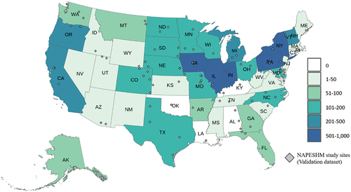
A soil health dataset was compiled from 7,232 soil samples (0–15 cm depth) from across the continental U.S. that were collected and analyzed between 2015 and 2019 (Figure 1; Table S1). The dataset was derived from routine soil sample submission to the Cornell Soil Health Laboratory. While all regions of the continental U.S. were represented in the Training Dataset, most samples derived from the Midwest, Northeast, Mid-Atlantic, and Northern Plain regions (Figure 1; Table S1; Figure S1). Soil samples were, per guidelines, assumed to have been collected by composing five or more soil slices (0-to-15 cm depth) from different locations in a field or plot (Cornell Soil Health Laboratory 2022). Samples were analyzed for soil texture and a suite of physical, biological, and chemical soil health indicators according to the CASH protocol (Moebius-Clune et al. 2017). Therefore, all samples contained measurements for the following co-variate properties that were used in this analysis: sand, silt, clay, wet aggregate stability (WAS), SOM, permanganate oxidizable carbon (POXC), soil respiration (Resp), and Modified Morgan extractable K, Mg, Fe, and Mn. Previous AWC RF model development determined that pH, P, and Zn added little predictability to the model and therefore were not included as predictor variables (Amsili, Van Es, and Schindelbeck 2022). Additionally, field capacity (θ_FC) and permanent wilting point (θ_PWP), which are not reported in CASH, but are used to calculate AWC, were aggregated with this dataset. Soils with SOM values greater than 10.0% were removed from the dataset to develop models that are appropriate for mineral agricultural soils. All soil analysis procedures are described in Schindelbeck et al. (2022).

Figure 1. Distribution of soil samples by state across the continental U.S. within the training dataset for field capacity, permanent wilting point, and available water capacity pedotransfer functions. Soil samples from NAPESHM study sites within the U.S. were used as the validation dataset to test models.

Analysis of physical properties

Soil texture was measured using a rapid and quantitative texture method that uses 3% sodium hexametaphosphate and shaking to disperse soil particles. Then, samples are sieved through 53 µm and allowed to sediment for two hours to determine the percentage of sand, silt, and clay (Kettler, Doran, and Gilbert 2001). WAS was measured by shaking soil samples for 10 s on a mechanical shaker with stacked sieves of 2.0 and 0.25 mm to collect macroaggregates between 0.25-to-2.0 mm. A single layer of macroaggregates was spread on a 0.25 mm mesh sieve and received 1.25 cm of water and 2.5 J of energy over a 5-min period. WAS was determined as the fraction of stable soil that remains above the sieve, correcting for particles >0.25 mm. θ_FC and θ_PWP were measured by placing approximately 15 g of air dried-2 mm-sieved soil into rubber rings on 1 and 15 bar porous ceramic pressure plates, respectively, and allowing soils to completely saturate (Soil Moisture Equipment Corp., Goleta, CA). Then pressure plates were placed in pressure chambers and equilibrated to −10 kPA (θ_FC) and −1500 kPA (θ_PWP). Field capacity water content was chosen to be at −10 kPa instead of the more commonly used −33 kPa because (i) most soils under consideration have limited depth to restricting layers or water tables (Fan, Li, and Miguez-Macho 2013; Reynolds and Topp 2008a), and (ii) plant water availability is most critical during growing seasons when water uptake is immediate after soil recharge (rather than after a 2–3 day drainage period). Field capacity is also defined as −10 kPa in Australia, New Zealand, Sweden, and by Ward Labs in the US (Nemes, Pachepsky, and Timlin 2011; Robertson et al. 2021; Ward 2021). AWC was calculated as the difference in gravimetric water content between θ_FC and θ_PWP (Reynolds and Topp 2008b).

Analysis of biological properties

SOM was analyzed by mass loss on ignition (LOI) in a muffle furnace at 500°C for two hours. Then % LOI was converted to % SOM using Equation 1(1) $\%\mathit{SOM}=\left(\%\mathit{LOI}\times 0.7\right)-0.23$(1) from Storer (1984), which is the standard method for calculating % SOM in New York State.

(1) $\%\mathit{SOM}=\left(\%\mathit{LOI}\times 0.7\right)-0.23$(1)

POXC was measured in duplicate, by reacting 2.5 g of soil with 20 mL 0.02 M potassium permanganate (KMnO₄) x 0.1 M calcium chloride (CaCl₂) solution (pH 7.2). Extracts were shaken for 2 minutes at 120 rpm and then allowed to settle for exactly 8 minutes. An aliquot of solution was diluted 100-fold and absorbance readings were taken at 550 nm using a handheld spectrophotometer (Hach, Loveland, CO). Absorbance was converted to mg POXC per kg soil using the equation of Weil et al. (2003) and a standard curve. Resp was analyzed by measuring cumulative CO₂ production over a four-day incubation with an alkali trap on 20.0 g air dried-8 mm sieved soil sample. The amount of CO₂ produced and absorbed by the KOH trap over the course of incubation was determined by measuring the change in electrical conductivity of the solution with an OrionTM DuraProbeTM 4-Electrode Conductivity Cell (ThermoFisher Scientific, Inc., Waltham, MA). Blanks without soil were also incubated to subtract CO₂ from the air that reacted with the alkali trap (Nunes et al. 2018).

Analysis of chemical properties

Nutrients were measured by extracting soil with a Modified Morgan solution (ammonium acetate plus acetic acid, pH 4.8) and then extracts were analyzed using inductively coupled plasma optical emission spectrometry (SPECTRO Analytical Instruments Inc., Mahwah, NJ) (Wolf and Beegle 1995). All nutrient contents are reported in units of mg kg⁻¹ soil (ppm).

Validation dataset

The North American Project to Evaluate Soil Health Measurements (NAPESHM; Norris et al. 2020) data were used as an independent validation dataset to test the accuracy of developed pedotransfer functions for θ_FC, θ_PWP, and AWC. The NAPESHM validation dataset contained 1,406 composite soil samples that were collected within the US, from 0 to 15 cm depth, in 2019 (Figure 1; Table S2). The project, conducted by the Soil Health Institute (Cary, NC), sampled 90 long-term (>10 years) experiments that were testing treatments from various agronomic management practices, including tillage, nutrient management, cover crops, crop diversity, water management, or multiple stacked practices (Norris et al. 2020; Figure 1). Samples were submitted to the Cornell Soil Health Laboratory for the analysis of all soil properties using the same methods in the training dataset: sand, silt, clay, θ_FC, θ_PWP, AWC, WAS, SOM, POXC, Resp, and Modified Morgan K, Mg, Fe, and Mn (Norris et al. 2020). The Training and NAPESHM datasets had similar distributions of sand, silt, and clay. However, the Training dataset had a slightly higher mean SOM value and a larger proportion of samples with SOM values between 4 and 8% than the NAPESHM dataset (Figure S2). The NAPESHM Validation Dataset provides a completely independent dataset to validate pedotransfer functions developed with the Training Dataset.

The NAPESHM dataset was also used to determine if model predictions could be equally sensitive to management as the measured values. We selected 57 experiments with at least 12 experimental plots, which included 1,178 observations, and assessed the sensitivity of measured gravimetric AWC to management. Treatments depended on the experiment but included at least one of the following treatment factors: tillage, cover crop, nutrient type, nutrient rate, cropping category (i.e., row crop, perennial, etc.), residue removal, crop rotation, and landscape position. In experiments where treatments had a significant effect on gravimetric AWC, we investigated whether modeled predictions could replicate those results. Gravimetric AWC model predictions included direct RF model predictions of AWC or calculation of AWC through separate RF prediction of θ_FC and θ_PWP.

Modeling approaches

Multiple linear regression

Multiple linear regression (MLR) models for θ_FC, θ_PWP, and AWC were fit to the Training dataset using sand, clay, and SOM, which are the most widely used to develop MLR pedotransfer functions for θ_FC and θ_PWP (Bagnall et al. 2022; Saxton and Rawls 2006). For θ_FC and AWC, MLR models included coefficients for sand, clay, SOM, sandxclay, sandxSOM, and clayxSOM. Whereas θ_PWP MLR models only included coefficients for sand, clay, and SOM. MLR models were fit using the lm function in R (R Core Team 2022), and nonsignificant coefficients were underlined in MLR Equations.

Random forest machine learning algorithm

Random forest is a robust non-linear machine learning algorithm that combines predictions of many decision trees (a forest) to model variables. Each decision tree is made with a bootstrap sample (random sampling with replacement) of approximately 63.2% of the Training Dataset. In each tree, a random subsample of all predictor variables, p, is tested as the splitting variable that will minimize error at various nodes in the tree (Breiman 2001; Liaw and Wiener 2002). The out-of-bag (OOB) samples, or the 36.8% that are omitted from building the decision tree, are predicted on that decision tree. RF predictions take the average of predictions of each decision tree in the forest. Aggregated OOB predictions are used to test and validate the predictions from the RF model (Liaw and Wiener 2002). Unlike MLR, RF allows for many predictor variables to be used without the effects of less important predictor variables being masked by more important predictor variables. Additionally, RF can capture non-linear or local importance of predictor variables. RF models were run using the randomForest package in R, which implements Breiman’s random forest algorithm (Breiman 2001; Liaw and Weiner 2022). Seed was arbitrarily set at 500 using the set.seed function in R to make the RF models reproducible. Previous work determined that changing the set.seed parameter leads to insignificant changes to the RF models. An exercise with one Full RF model in this study showed that changing the set.seed parameter led to insignificant increases of only 0.26%, 0.29%, and 0.80% from the min to max values of percent variance explained, OOB RMSE, and RMSE, respectively. The parameters for each RF model were: 500 trees, randomForest defaults (mtry = p/3, rounded down; target node size = 5), proximity = TRUE, localImp = TRUE.

Full and Reduced RF models were developed for θ_FC, θ_PWP, and AWC. The Full RF models used all available predictor variables, which included sand, silt, clay, WAS, SOM, POXC, Resp, and Modified Morgan K, Mg, Fe, and Mn. Whereas the Reduced RF models used sand, silt, clay, and SOM. Full and Reduced RF models were compared to determine how novel variables contribute to the prediction of θ_FC, θ_PWP, and AWC.

Pedotransfer function validation

Initial validation of pedotransfer functions was done with the Training Dataset by plotting predictions against measured values. For the RF models, percent of variance (%Var) explained and OOB root mean square error (RMSE) and OOB normalized RMSE (NRMSE) were calculated. %Var explained is a metric provided with RF models in R and can be described as how well the OOB predictions match the observed values (Equation 2(2) $\%\mathit{Var}\mathit{Explained}=\left(1-\frac{MSEofOOBp\mathrm{redictions}:\frac{1}{n}{\sum }_{i=1}^n{\left(Y_i-{\hat{Y}}_{\mathit{i}}\right)}^2}{\mathit{Variance}\mathit{of}\mathit{observed}\mathit{values}:\frac{\sum {(x_i-\bar{x})}^2}{\mathit{n}-1}}\right)\times 100$(2) ). Therefore, it is a pseudo-R-squared metric defined by:

(2) $\%\mathit{Var}\mathit{Explained}=\left(1-\frac{MSEofOOBp\mathrm{redictions}:\frac{1}{n}{\sum }_{i=1}^n{\left(Y_i-{\hat{Y}}_{\mathit{i}}\right)}^2}{\mathit{Variance}\mathit{of}\mathit{observed}\mathit{values}:\frac{\sum {(x_i-\bar{x})}^2}{\mathit{n}-1}}\right)\times 100$(2)

Out of bag (OOB) RMSE was calculated by comparing OOB model predictions to measured values:

(3) $\mathit{RMSE}=\sqrt{\frac{1}{n}{\sum }_{i=1}^n{\left(Y_i-{\hat{Y}}_{\mathit{i}}\right)}^2}$(3)

The OOB NRMSE was calculated by dividing the OOB RMSE by the average of the measured values:

(4) $\mathit{NRMSE}=\frac{\sqrt{\frac{1}{n}{\sum }_{i=1}^n{\left(Y_i-{\hat{Y}}_{\mathit{i}}\right)}^2}}{\overline{Y_i}}$(4)

For MLR models, adjusted R², RMSE (Equation 3(3) $\mathit{RMSE}=\sqrt{\frac{1}{n}{\sum }_{i=1}^n{\left(Y_i-{\hat{Y}}_{\mathit{i}}\right)}^2}$(3) ), and NRMSE (Equation 4(4) $\mathit{NRMSE}=\frac{\sqrt{\frac{1}{n}{\sum }_{i=1}^n{\left(Y_i-{\hat{Y}}_{\mathit{i}}\right)}^2}}{\overline{Y_i}}$(4) ) were calculated.

A secondary validation step was carried out with the NAPESHM data. Regression equations, mean absolute error (MAE; Equation 5(5) $\mathit{MAE}=\frac{1}{n}{\sum }_{i=1}^n\left|Y_i-{\hat{Y}}_{\mathit{i}}\right|$(5) ), RMSE, and NRMSE were all used as validation metrics in the secondary validation step:

(5) $\mathit{MAE}=\frac{1}{n}{\sum }_{i=1}^n\left|Y_i-{\hat{Y}}_{\mathit{i}}\right|$(5)

Variable importance and partial dependence of RF models

RF models containing 100s of decision trees are more difficult to interpret (black-box) than a single decision tree, which can be easily visualized, or a MLR model with explicit coefficients. Several powerful tools have been developed to interpret RF models and variable importance. The randomForestExplainer package in R enables the calculation and visualization of the mean minimal depth (min_depth_distribution function), or the average location of predictor variables across all decision trees, where 0 is the root node of the tree, 1 is the 2^nd layer, etc (Palusynska, Biecek, and Jiang 2022). It also extracts variable importance metrics from the RF model, including MSE increase, which ranks variables by their ability to reduce mean square error of the prediction (i.e., higher MSE increase values are associated with more predictive variables), and node purity increase, how much each variable improves the purity of different parts of the tree (Palusynska, Biecek, and Jiang 2022). Additionally, Shapley Additive exPlanations (SHAP) values were calculated and visualized using the kernalshap and shapviz packages in R, respectively (Mayer and Stando 2023; Mayer, Watson, and Prezemyslaw 2023). SHAP is a popular technique for interpreting machine learning models due to its flexibility (i.e., can be used on any machine learning model, which is useful for model comparison) and ability to predict individual predictions (Molnar 2023). SHAP values calculate variable importance by comparing model predictions with and without the variable of interest (Tseng 2018). SHAP values were calculated using the kernalshap function with 1,085 random samples from the training dataset to explain (number picked within the recommended range) and 362 random samples from the training dataset as background (number picked within the recommended range) (Mayer, Watson, and Prezemyslaw 2023). Then, two types of sv importance plots were constructed: a simple one that showed the mean absolute SHAP value, which can be interpreted as the magnitude of the effect of each variable on the predicted value; and a “beeswarm” plot, which plots each of the SHAP values of those 1,085 points and maps each predictor variable value from high to low.

Partial dependence analysis with the pdp package was used to determine the influence of single predictor variables on θ_FC, θ_PWP, and AWC in the full RF models, while other variables are held constant. The four most important predictor variables for θ_FC, θ_PWP, and AWC as indicated by the MSE increase metric were run as individual partial dependence plots. The next three most important variables (i.e., 5^th − 7^th) were included in the supplemental materials for θ_FC and AWC. The pdp package also provides functionality to plot multi-predictor partial dependence plots (Greenwell 2017) which were constructed with SOM and sand or clay to visualize interaction among those variables. Variable importance and partial dependence plots were only made for the full RF models for θ_FC, θ_PWP, and AWC.

Results and discussion

Field capacity (θ_FC)

Model comparison and validation

Three pedotransfer functions were developed for gravimetric θ_FC, including a Full RF model, a Reduced RF model, and MLR (Equation 6(6) ${\theta }_{\mathit{FC}}=0.3477-0.313\mathit{sand}+0.040\mathit{clay}+1.855\mathit{SOM}+0.222\left(\mathit{sand}\times \mathit{clay}\right)+1.405\left(\mathit{sand}\times \mathit{SOM}\right)-0.202\left(\mathit{clay}\times \mathit{SOM}\right)$(6) ). Units of predictor variables and θ_FC in Equation 6(6) ${\theta }_{\mathit{FC}}=0.3477-0.313\mathit{sand}+0.040\mathit{clay}+1.855\mathit{SOM}+0.222\left(\mathit{sand}\times \mathit{clay}\right)+1.405\left(\mathit{sand}\times \mathit{SOM}\right)-0.202\left(\mathit{clay}\times \mathit{SOM}\right)$(6) are in g g⁻¹ (i.e., g H₂O g⁻¹ oven dry soil and g sand g⁻¹ oven dry soil).

(6) ${\theta }_{\mathit{FC}}=0.3477-0.313\mathit{sand}+0.040\mathit{clay}+1.855\mathit{SOM}+0.222\left(\mathit{sand}\times \mathit{clay}\right)+1.405\left(\mathit{sand}\times \mathit{SOM}\right)-0.202\left(\mathit{clay}\times \mathit{SOM}\right)$(6)

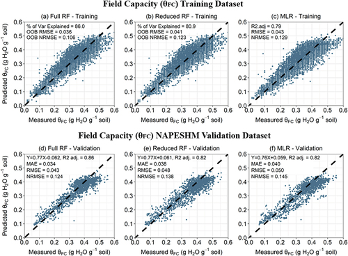
The first validation step with the Training dataset revealed that the Full RF model had the highest percent variance explained (86.0%) and lowest RMSE (0.036) compared to the Reduced RF (%Var explained = 80.9%; RMSE = 0.042) and MLR models (R²_adj = 0.79; RMSE = 0.043; Figure 2a–c). Furthermore, the Reduced RF model had a similar percent variance explained and RMSE to the MLR model (Figure 2b,c). The second validation step with the independent NAPESHM dataset reinforced trends among models found using the Training dataset (Figure 2d–f). It also demonstrated that each model had NRMSEs that were on average 13.9% higher (Reduced RF: 12.2%, MLR: 12.4%, and Full RF: 17.0%) than the same model calculated for the Training dataset (Figure 2). Therefore, although RF is robust against overfitting (Breiman 2001), the RF models displayed a similar amount of overfitting to the Training dataset as the MLR model. Another explanation for the deviation in performance between Training and NAPESHM Validation datasets is that the Training Dataset had proportionally fewer samples from the Southern Plain States and Northwest than the NAPESHM dataset (Tables S1 and S2). The Full RF model had a 16.3% lower RMSE than the MLR model, which indicates inclusion of additional variables beyond sand, silt, clay, and SOM can provide meaningful improvements to prediction of θ_FC (Figure 2d–f). In contrast, we found that the Reduced RF model performed similarly to the MLR model that contained similar predictor variables: sand, silt, clay, and SOM, indicating that simple modeling approaches like MLR can be adequate in situations where only 3–4 predictor variables are being used. If the goal is prediction and access is available to many potential predictors of θ_FC, machine learning algorithms, like RF, can utilize all those variables to improve the prediction of θ_FC.

Figure 2. (a-c) measured vs. predicted field capacity water content (θ_FC) for full random forest (RF), reduced RF, and multiple linear regression (MLR) models on the training dataset. (a-b) full and reduced RF models show out of bag predictions. Validation metrics within plots include percent variance explained, out of bag (OOB) root mean square error (RMSE), and OOB normalized RMSE (NRMSE). (d-f) measured vs. predicted field capacity for full RF, reduced RF, and MLR models for the NAPESHM validation dataset. Text within plots includes the regression equation, adjusted R², mean absolute error (MAE), RMSE, and NRMSE.

Variable importance

Variable importance approaches for the Full RF θ_FC model showed that sand was the most influential predictor variable, followed by SOM and silt, and then clay (Figures 3 and S3). By the nature of its particle diameter (53–2,000 µm), sand content is the primary determinant of the percentage of total porosity with a pore diameter equal to or smaller than 30 µm, which is the theoretical pore size that is drained at −10 kPa or θ_FC (Amer, Logsdon, and Davis 2009; Moebius et al. 2007). Therefore, there was a strong negative relationship between sand content and θ_FC (Figure 3a). Both silt and SOM were of secondary importance as predictor variables of θ_FC. Silt was slightly more important than SOM for improving the prediction of θ_FC as indicated by a larger MSE increase value (Figure S3b), but both had similar magnitude effects on θ_FC (Figure S3c). Clay content was the least important of the four variables as indicated by MSE increase and mean SHAP values (Figure S3). Interestingly, there was an interaction between sand content and SOM, where increases in SOM led to larger increases in θ_FC between 50 to 100% sand (coarser-textured) than between 0 to 25% sand (finer-textured). This corroborates similar findings that AWC responds to SOM to a larger extent in sandier soils than in silty or clayey soils (Bauer and Black 1992; Libohova et al. 2018; Minasny and Mcbratney 2018).

Figure 3. (a-d) partial dependence plots for individual field capacity water content (θ_FC) predictor variables: sand, silt, clay, and soil organic matter. (e) Multi-predictor partial dependence plot with the interaction between sand and soil organic matter. These partial dependence plots show the influence of individual predictor variables on θ_FC within the full RF model while all other predictor variables are held constant.

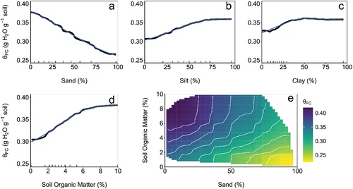
After sand, silt, SOM, and clay, POXC, Mg, and K were the next three most important variables for improving the prediction of θ_FC as indicated by MSE increase and mean SHAP metrics (Figure S3). Higher values for POXC, Mg, and to a lesser extent K were associated with higher values for θ_FC (Figure S4). POXC provides redundancy in the model and likely helps to capture the effects of increasing SOM content on θ_FC. Extractable Mg could potentially indicate soils that have calcareous mineralogy, which can influence soil water retention (Bagnall et al. 2022). Extractable Mg and to a lesser extent K show negative correlations with sand content and positive correlations with SOM content (Amsili, Van Es, and Schindelbeck 2021), which indicates that they may also provide some redundancy for sand and SOM effects on θ_FC.

Permanent wilting point (θ_PWP)

Model comparison and validation

Three pedotransfer functions were developed for gravimetric θ_PWP, including a Full RF model, a Reduced RF model, and MLR (Equation 7(7) ${\mathit{\theta }}_{\mathit{P}\mathrm{WP}}=0.0132-0.014\mathit{sand}+0.244\mathit{clay}+1.158\mathit{SOM}$(7) ). Units of predictor variables and θ_PWP in Equation 7(7) ${\mathit{\theta }}_{\mathit{P}\mathrm{WP}}=0.0132-0.014\mathit{sand}+0.244\mathit{clay}+1.158\mathit{SOM}$(7) are in g g⁻¹.

(7) ${\mathit{\theta }}_{\mathit{P}\mathrm{WP}}=0.0132-0.014\mathit{sand}+0.244\mathit{clay}+1.158\mathit{SOM}$(7)

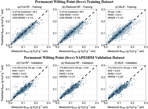
There were fewer differences among models for θ_PWP then among models for θ_FC when they were compared using the Training (Figure 4a–c) and Validation Datasets (Figures 2 and 4d–f). The Full RF model had a higher percent variance explained (92.3%) and lower RMSE (0.011) compared to the MLR model (R²_adj = 0.88; RMSE = 0.013) but was only marginally better than the Reduced RF model (%Var explained = 89.7%; RMSE = 0.012; Figure 4a–c). The second validation step with the independent NAPESHM dataset illustrated once again that each model had NRMSEs that were on average 36.3% higher (MLR: 28.9%, Reduced RF: 33.1%, and Full RF: 46.9%) than the same model calculated for the Training dataset (Figure 4). As before, this demonstrates that RF models can be just as susceptible to overfitting to the Training dataset as an MLR model. The Full RF model had a 13.3% lower RMSE than the MLR model, which indicates that RF models can provide slight improvements to the prediction of θ_PWP (Figure 4d–f). In contrast to the prediction of θ_FC, the Full RF model was only marginally better than the Reduced RF model, which indicates that additional predictor variables provide less benefit for predicting θ_PWP than θ_FC, i.e., it is mostly defined by texture and SOM.

Figure 4. (a-c) measured vs. predicted permanent wilting point water content (θ_PWP) for full random forest (RF), reduced RF, and multiple linear regression (MLR) models on the training dataset. (a-b) full and reduced RF models show RF model out of bag predictions. Validation metrics within plots include percent variance explained, out of bag (OOB) root mean square error (RMSE), and OOB normalized RMSE (NRMSE). (d-f) measured vs. predicted permanent wilting point for full RF, reduced RF, and MLR models for the NAPESHM validation dataset. Text within plots includes the regression equation, adjusted R², mean absolute error (MAE), RMSE, and NRMSE.

Variable importance

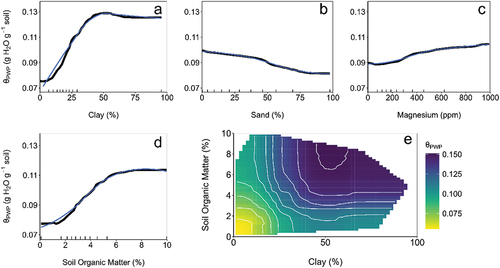
Clay was the most important variable for the prediction of θ_PWP, followed by SOM, and then Mg and sand (Figure 5, Equation 7(7) ${\mathit{\theta }}_{\mathit{P}\mathrm{WP}}=0.0132-0.014\mathit{sand}+0.244\mathit{clay}+1.158\mathit{SOM}$(7) , Figure S5). Clay content’s importance in predicting PWP is sensible because clay is the primary determinant of the proportion of total porosity with a pore diameter equal to less than 0.20 µm, which is the theoretical pore size that can hold water at −1500 kPA (Amer, Logsdon, and Davis 2009). As follows, there was a strong positive relationship between clay content and θ_PWP from 0 to approximately 40% clay (Figure 5a). SOM also had a positive influence on θ_PWP from between 0 to approximately 7%, which may be due to an increase in total porosity or an increase in the proportion of total porosity with a diameter less than 0.20 µm (Libohova et al. 2018). SOM had a smaller effect on θ_PWP (Figure 5d) than it does on θ_FC (Figure 3d) by approximately a magnitude of 2. Both sand and exchangeable Mg led to similar reductions in MSE of θ_PWP and had similar size effects on θ_PWP. Sand had a negative effect on θ_PWP (Figure 5b) because increases result in a smaller proportion of total porosity with a diameter less than 0.20 µm. Whereas, Mg had a slight positive effect on θ_PWP, which could potentially be helping to separate soils that have clay mineralogy with more surface area like smectites (Figure 5c; Chu and Johnson 1985). This is a novel finding that extractable Mg was equally important to sand for the prediction of θ_PWP. Unlike θ_FC, there was no clear interaction between clay content and SOM, which was counter to previous research that found that SOM had a smaller impact on θ_PWP in soils with higher clay content (Minasny and Mcbratney 2018; Saxton and Rawls 2006). Further variables were not explored due to the similarity between full and reduced RF models (i.e., texture components and SOM were sufficient for predicting θ_PWP).

Figure 5. (a-d) partial dependence plots for individual permanent wilting point water content (θ_PWP) predictor variables: clay, sand, magnesium, and soil organic matter. (e) Multi-predictor partial dependence plot with the interaction between clay and soil organic matter. These partial dependence plots show the influence of individual predictor variables on θ_PWP within the full RF model while all other predictor variables are held constant.

Available water capacity (AWC)

Model comparison and validation

Three pedotransfer functions were developed for gravimetric AWC, including a Full RF model, a Reduced RF model, and MLR (Equation 8(8) $\mathit{AWC}=0.340-0.304\mathit{sand}-0.212\mathit{clay}+0.526\mathit{SOM}+0.184\left(\mathit{sand}\times \mathit{clay}\right)+1.708\left(\mathit{sand}\times \mathit{SOM}\right)-0.153\left(\mathit{clay}\times \mathit{SOM}\right)$(8) ). Units of predictor variables and AWC in Equation 8(8) $\mathit{AWC}=0.340-0.304\mathit{sand}-0.212\mathit{clay}+0.526\mathit{SOM}+0.184\left(\mathit{sand}\times \mathit{clay}\right)+1.708\left(\mathit{sand}\times \mathit{SOM}\right)-0.153\left(\mathit{clay}\times \mathit{SOM}\right)$(8) are in g g⁻¹.

(8) $\mathit{AWC}=0.340-0.304\mathit{sand}-0.212\mathit{clay}+0.526\mathit{SOM}+0.184\left(\mathit{sand}\times \mathit{clay}\right)+1.708\left(\mathit{sand}\times \mathit{SOM}\right)-0.153\left(\mathit{clay}\times \mathit{SOM}\right)$(8)

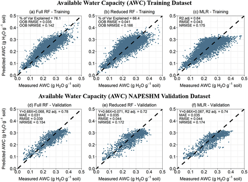
Similar to θ_FC, the Full RF model performed better for AWC (%Var explained = 75.4%; RMSE = 0.035) than the Reduced RF and MLR models with the Training Dataset (Figure 6a–c). Whereas the Reduced RF model only had a marginally higher percent variance explained (66.4%) and marginally lower RMSE (RMSE = 0.041) than the MLR model (R²_adj = 0.64; RMSE = 0.043; Figure 6b,c). The secondary independent validation with the NAPESHM dataset revealed that the Reduced RF and MLR models performed similarly (Figure 6e,f). It also demonstrated that each model had NRMSEs that were on average 3.8% higher (MLR: −0.6%, Reduced RF: 3.6%, and Full RF: 8.5%) than the same model calculated for the Training dataset (Figure 6). In contrast to the models for θ_FC and θ_PWP, the models for AWC performed similarly when compared between the Training and Validation datasets. The Full RF model had a 12.8% lower RMSE than the MLR model, which indicates inclusion of additional variables beyond sand, silt, clay, and SOM can provide meaningful improvements to prediction of AWC (Figure 6d–f). In contrast, we found that the Reduced RF model performed similarly to the MLR model that contained similar predictor variables: sand, silt, clay, and SOM, indicating that simple modeling approaches like MLR can be adequate in situations where only 3–4 predictor variables are being used. If the goal is prediction and many potential predictors are available from a standard test, machine learning algorithms like RF can utilize all those variables to improve the prediction of AWC.

Figure 6. (a-c) measured vs. predicted available water capacity (AWC) for full random forest (RF), reduced random forest, and multiple linear regression models on the training dataset. (a-b) full and reduced random forest models show OOB RF model predictions on the training dataset. Validation metrics within plots include percent variance explained, out of bag (OOB) root mean square error (RMSE), and OOB normalized RMSE (NRMSE). (d-f) measured vs. predicted available water capacity for full random forest, reduced random forest, and multiple linear regression models for the NAPESHM validation dataset. Text within plots includes the regression equation, adjusted R², mean absolute error (MAE), RMSE, and NRMSE.

Variable importance

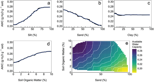
Silt and sand were the most important variables for predicting AWC, followed by SOM, clay, and POXC (Figures 7 and S6b). Silt was slightly more useful for reducing the MSE and had a slightly larger impact on AWC values than sand (Figures 6b,c and S6b,c). Silt content’s importance for predicting AWC may be related to its particle size diameter range, 2–53 µm, corresponding most closely to the theoretical pore size range that stores plant available water, 0.20–30 µm (Amer, Logsdon, and Davis 2009; Libohova et al. 2018). Previous studies have documented that silt content has the highest correlation with AWC, followed by sand content (Amsili, Van Es, and Schindelbeck 2021; Libohova et al. 2018). Silt has a positive relationship with AWC while sand has a negative relationship with AWC. As described above, as sand content increases, the proportion of total porosity with a pore diameter greater than 30 µm, which is drained at −10kPa or θ_FC, increases. SOM, clay, and POXC were the third, fourth, and fifth most important variables for reducing MSE in the RF model. Both SOM and POXC had positive impacts on AWC values, with SOM having a slightly stronger influence on AWC than POXC as indicated by its mean SHAP value (Figures 7d, S6c and S7a). There was a clear interaction between sand content and SOM, where SOM has a larger effect on AWC in soils with higher sand content (Figure 7e). This interaction is visible in partial dependence plots for individual soil texture classes, where changes in SOM from 0 to 6% caused increases in AWC of 0.054, 0.051, 0.032, and 0.029 g H₂O g⁻¹ soil for sandy loam, loam, silt loam, and clay loam, respectively (Figure S8). Previous research has documented similar interactions between sand and SOM content (Libohova et al. 2018; Minasny and Mcbratney 2018; Rawls et al. 2003). The importance of POXC in the model indicates that POXC provides some additional value to SOM in prediction of AWC. POXC represents a small fraction of the total SOC by mass (i.e. 1–6% of total SOC; Amsili et al. 2023, unpublished data) and has been determined to most closely represents phenolic and polyphenolic compounds (Christy et al. 2023). Therefore, POXC likely provides some redundancy for SOM and may help to capture SOM quality effects on AWC. Although clay helped reduce MSE in the model, it had a negligible effect on AWC values as indicated by its partial dependence plot (Figure 7c) and mean SHAP value (Figure S6c). Interestingly, WAS and extractable Fe had a greater impact on AWC values in the RF model than clay content (Figure S7b,c). Higher WAS values were associated with lower AWC values (Figures S6c and S7b) which is likely an artifact of the WAS method used that tends to result in slightly higher mean values for coarse-textured soils compared to loam and fine-textured soils (Amsili et al. 2023). Extractable Fe also had a positive impact on AWC, which could help to parameterize pastures and hayfields, which tend to have lower pHs and as a result higher extractable Fe (Amsili, Van Es, and Schindelbeck 2021).

Figure 7. (a-d) partial dependence plots for individual available water capacity (AWC) predictor variables: sand, silt, clay, and soil organic matter. (e) Multi-predictor partial dependence plot with the interaction between sand and soil organic matter. These partial dependence plots show the influence of individual predictor variables on AWC within the full RF model while all other predictor variables are held constant.

Sensitivity of AWC and RF models to agronomic management

Laboratory-measured gravimetric AWC was sensitive to treatment effects (p < .05) at 23/57 sites that were analyzed but was not consistently sensitive to specific agronomic management practices. Three of those significant results were not easily explainable by the associated SOM or texture data. Crop rotation, nutrient type, residue return level, tillage, cropping system, and cover crops significantly affected gravimetric AWC at 30.0, 28.6, 28.6, 26.8, 20.0, and 14.3% of sites that tested those management practices. Additionally, soil texture class did not appear to influence whether gravimetric AWC was sensitive to management. Gravimetric AWC was sensitive to management in 50, 30, 36, 40, 43, and 67% of loamy sand, sandy loam, loam, silt loam, clay loam, and silty clay loam sites, respectively. This potentially does not support the result that management is more likely to have a positive effect on AWC in coarser-textured soils, as is indicated in the model and previous research (Libohova et al. 2018; Minasny and Mcbratney 2018; Rawls et al. 2003). However, the duration of the experiment influenced the likelihood that agronomic management had a significant effect on gravimetric AWC. For example, only 18% of the experiments running for 0–15 years showed significant results. Whereas 75% of the experiments running for >45 years had significant results. This relatively short-term insensitivity to agronomic management may be an inherent limitation with gravimetric AWC as a dynamic soil health indicator. Using intact soil cores to measure θ_FC shows greater response to agronomic management but involves a significantly more expensive measurement that is not practical for routine laboratory analysis (Bagnall et al. 2022).

Prediction of AWC directly or calculation of AWC with predicted θ_FC and θ_PW using full RF models was able to replicate significant (p < .05) results at 5/20 sites when excluding apparent nonsensical results. However, at p < .10 AWC from predicted θ_FC and θ_PWP was able to accurately predict more experiments (9/20) than direct prediction of AWC (6/20). This suggests a slight advantage of predicting AWC by calculating it from predicted θ_FC and θ_PWP rather than direct prediction of AWC. In contrast, the direct prediction of AWC had a similar RMSE to the calculation of AWC with predicted θ_FC and θ_PWP (0.0389 vs 0.0395; Figure S9), indicating that a single Full RF model of AWC can enable direct prediction for use by a high throughput lab. Therefore, both methods of prediction of AWC are valid and up to the discretion of the user.

Comparison of predicted and measured AWC in long-term experiments demonstrated that using an RF model loses some statistical power to detect treatment effects compared to laboratory measured AWC. This is in part explained by the fact that sustainable agronomic management practices generally result in increased SOM, but this is associated with higher values for both θ_FC (Figure 3d) and θ_PWP (Figure 5d), thereby resulting in only modest effects on AWC = θ_FC-θ_PWP (Figure 7d; Libohova et al. 2018). In all, AWC is best regarded as a relevant inherent soil property with limited ability to measure dynamic change, or soil health effects, from agronomic management.

Model availability and use

Full and reduced RF model files for θ_FC, θ_PWP, and AWC (i.e., six models) are available for download at the Harvard Dataverse (Amsili, Van Es, and Schindelbeck 2022). The Training dataset used to calibrate the models developed in this study is available for download. The Full RF model for AWC is most precise (lowest RMSE) in the Southwest, Southeast, and Northeast & Lake States, and least precise (highest RMSE) in the southern Plain States and Northwest (Figure S10). This is in part explained by less representation of these regions in the Training dataset, although the Southwest and Southeast also had low sample numbers but had high model performance (Table S1; Figure S10). New pedotransfer functions for gravimetric AWC fit into existing interpretive frameworks and cumulative normal distribution functions for scoring AWC, which would enable their rapid implementation by a commercial soil health laboratory (Moebius-Clune et al. 2017).

Conclusions

Growing interest in comprehensive soil health assessment requires the development of pedotransfer functions to predict some of the costly soil health indicators instead of directly measuring them. Gravimetric AWC is widely considered a key physical soil health measurement and the only indicator to directly assess a soil’s water supply capacity. However, of the commonly measured soil health indicators, it is the most time-intensive, expensive to measure, and least sensitive to management. Our research utilizing large training and validation datasets demonstrated that full random forest models improved prediction of θ_FC, θ_PWP, and AWC compared to MLR models. This indicates that if the goal is prediction, variables beyond sand, silt, clay, and SOM such as POXC, WAS, and extractable Mg, K, and Fe can improve predictions of θ_FC, θ_PWP, and AWC. NAPESHM experiments confirmed that gravimetric AWC is not consistently sensitive to management practices that have been carried out for <30 years, indicating its short-term insensitivity. Therefore, gravimetric AWC is most useful for capturing a soil’s inherent ability to store plant available water and some dynamic effects of large differences in SOM on AWC, but is less useful for capturing the effects of short-term agronomic management on this function.

Abbreviations

θFC	=	gravimetric field capacity water content
θPWP	=	gravimetric permanent wilting point water content
AWC	=	available water capacity
WAS	=	wet aggregate stability
SOM	=	soil organic matter
SOC	=	soil organic carbon
Resp	=	soil respiration from 4-day incubation
POXC	=	permanganate-oxidizable carbon
CASH	=	Comprehensive Assessment of Soil Health
NAPESHM	=	North American Project to Evaluate Soil Health Measurements
RF	=	random forest
OOB	=	out-of-bag
MLR	=	multiple linear regression
RMSE	=	root mean square error
MAE	=	mean absolute error.

Acknowledgements

The authors want to acknowledge the staff of the Cornell Soil Health Laboratory who ensured high quality soil health assessment results: Kirsten Kurtz, Zach Batterman, Brianna Binkerd-Dale, Nate Baker, Bamidaaye Sinon, Akossiwoa Sinon, and Steven Dunn. The authors also want to acknowledge the Soil Health Institute for carrying out the North American Project to Evaluate Soil Health Measurements, which provided a robust and independent validation dataset to test pedotransfer functions for θ_FC, θ_PWP, and AWC.

Disclosure statement

No potential conflict of interest was reported by the author(s).

Supplementary material

Supplemental data for this article can be accessed online at https://doi.org/10.1080/00103624.2024.2336573

Additional information

Funding

This research was supported by a contract with the New York State Environmental Protection Fund, which was administered by the New York State Department of Agriculture and Markets. The North American Project to Evaluate Soil Health Measurements Dataset was part of a broader effort titled, “Assessing and Expanding Soil Health for Production, Economic, and Environmental Benefits” that was funded by the Foundation for Food and Agricultural Research (grant ID 523926), General Mills, and The Samuel Roberts Noble Foundation.

References

- Amer, A-M. M., S. D. Logsdon, and D. Davis. 2009. Prediction of hydraulic conductivity as related to pore size distribution in unsaturated soils. Soil Science 174 (9):508–15. doi:10.1097/SS.0b013e3181b76c29.
- Amsili, J. P., H. M. Van Es, D. M. Aller, and R. R. Schindelbeck. 2023. Empirical approach for developing production environment soil health benchmarks. Geoderma Regional 34:e00672. doi:10.1016/j.geodrs.2023.e00672.
- Amsili, J. P., H. M. Van Es, and R. R. Schindelbeck. 2021. Cropping system and soil texture shape soil health outcomes and scoring functions. Soil Security 4:100012. doi:10.1016/j.soisec.2021.100012.
- Amsili, J. P., H. M. Van Es, and R. R. Schindelbeck. 2022. An available water capacity pedotransfer function using random forest - 2020 cornell soil health model: Harvard Dataverse. https://dataverse.harvard.edu/dataset.xhtml?persistentId=doi:10.7910/DVN/U5DAEP.
- Andrews, S. S., D. L. Karlen, and C. A. Cambardella. 2004. The soil management assessment framework. Soil Science Society of America Journal 68 (6):1945–62. doi:10.2136/sssaj2004.1945.
- Araya, S. N., and T. A. Ghezzehei. 2019. Using machine learning for prediction of saturated hydraulic conductivity and its sensitivity to soil structural perturbations. Water Resources Research 55 (7):5715–37. doi:10.1029/2018WR024357.
- Bagnall, D. K., C. L. S. Morgan, M. Cope, G. M. Bean, S. Cappellazzi, K. Greub, and C. W. Honeycutt, C. L. Norris, E. Rieke, P. Tracy. 2022. Carbon-sensitive pedotransfer functions for plant available water. Soil Science Society of America Journal 86 (3):612–29. doi:10.1002/saj2.20395.
- Bauer, A., and A. L. Black. 1992. Organic carbon effects on available water capacity of three soil textural groups. Soil Science Society of America Journal 56 (1):248–54. doi:10.2136/sssaj1992.03615995005600010038x.
- Breiman, L. 2001. Random forests. Machine Learning 45 (1):5–32. doi:10.1023/A:1010933404324.
- Carranza, C., C. Nolet, M. Pezij, and M. Van Der Ploeg. 2021. Root zone soil moisture estimation with random forest. Journal of Hydrology 593:125840. doi:10.1016/j.jhydrol.2020.125840.
- Christy, I., A. Moore, D. Myrold, and M. Kleber. 2023. A mechanistic inquiry into the applicability of permanganate oxidizable carbon (poxc) as a soil health indicator. Soil Science Society of America Journal 87 (5):1083–95. doi:10.1002/saj2.20569.
- Chu, C.-H., and L. J. Johnson. 1985. Relationship between exchangeable and total magnesium in pennsylvania soils. Clays and Clay Minerals 33 (4):340–44. doi:10.1346/CCMN.1985.0330410.
- Cornell Soil Health Laboratory. 2022. Sample collection. https://soilhealthlab.cals.cornell.edu/testing-services/soil-sample-collection/.
- Fan, Y., H. Li, and G. Miguez-Macho. 2013. Global patterns of groundwater table depth. Science 339 (6122):940–43. doi:10.1126/science.1229881.
- Greenwell, B. M. 2017. Pdp: An r package for constructing partial dependence plots. The R Journal 9 (1):421–36. doi:10.32614/RJ-2017-016.
- Gupta, S. C., and W. E. Larson. 1979. Estimating soil water retention characteristics from particle size distribution, organic matter percent, and bulk density. Water Resources Research 15 (6):1633–35. doi:10.1029/WR015i006p01633.
- Idowu, O. J., H. M. Van Es, G. S. Abawi, D. W. Wolfe, R. R. Schindelbeck, B. N. Moebius-Clune, and B. K. Gugino. 2009. Use of an integrative soil health test for evaluation of soil management impacts. Renewable Agriculture and Food Systems 24 (3):214–24. doi:10.1017/S1742170509990068.
- Kettler, T. A., J. W. Doran, and T. L. Gilbert. 2001. Simplified method for soil particle-size determination to accompany soil-quality analyses. Soil Science Society of America Journal 65 (3):849–52. doi:10.2136/sssaj2001.653849x.
- Kinoshita, R., B. N. Moebius-Clune, H. M. Van Es, W. D. Hively, and A. V. Bilgilis. 2012. Strategies for soil quality assessment using visible and near-infrared reflectance spectroscopy in a western kenya chronosequence. Soil Science Society of America Journal 76 (5):1776–88. doi:10.2136/sssaj2011.0307.
- Kukal, M. S., S. Irmak, R. Dobos, and S. Gupta. 2023. Atmospheric dryness impacts on crop yields are buffered in soils with higher available water capacity. Geoderma 429:116270. doi:10.1016/j.geoderma.2022.116270.
- Liaw, A., and M. Weiner. 2022. Randomforest: Breiman and cutler’s random forests for classification and regression. R package version 4.7-1.1. https://cran.r-project.org/web/packages/randomForest/index.html.
- Liaw, A., and M. Wiener. 2002. Classification and regression by randomforest. R News 2 (3):18–22.
- Libohova, Z., C. Seybold, D. Wysocki, S. Wills, P. Schoeneberger, C. Williams, and P. R. Owens, D. Stott, P. R. Owens. 2018. Reevaluating the effects of soil organic matter and other properties on available water-holding capacity using the national cooperative soil survey characterization database. Journal of Soil and Water Conservation 73 (4):411–21. doi:10.2489/jswc.73.4.411.
- Mayer, M., and A. Stando. 2023. Shapviz: Shap visualizations. R package version 0.8.0. https://github.com/ModelOriented/shapviz.
- Mayer, M., D. Watson, and B. Prezemyslaw. 2023. Kernalshap: Kernal shap. R package version 0.3.7. https://github.com/ModelOriented/kernelshap.
- Minasny, B., and A. B. Mcbratney. 2018. Limited effect of organic matter on soil available water capacity. European Journal of Soil Science 69 (1):39–47. doi:10.1111/ejss.12475.
- Moebius-Clune, B. N., D. J. Moebius-Clune, B. K. Gugino, O. J. Idowu, R. R. Schindelbeck, A. J. Ristow, and G. S. Abawi. 2017. Comprehensive Assessment of Soil Health - the Cornell framework. Edition 3.2. Cornell University. Geneva, NY. http://soilhealth.cals.cornell.edu/training-manual/
- Moebius, B. N., H. M. Van Es, R. R. Schindelbeck, O. J. Idowu, D. J. Clune, and J. E. Thies. 2007. Evaluation of laboratory-measured soil properties as indicators of soil physical quality. Soil Science 172 (11):895–912. doi:10.1097/ss.0b013e318154b520.
- Molnar, C. 2023. Interpretable Machine Learning - a Guide for Making Black Box Models interpretable: Leanpub. https://christophm.github.io/interpretable-ml-book/
- Navidi, M. N., J. Seyedmohammadi, and S. A. Seyed Jalali. 2022. Predicting soil water content using support vector machines improved by meta-heuristic algorithms and remotely sensed data. Geomechanics and Geoengineering 17 (3):712–26. doi:10.1080/17486025.2020.1864032.
- Nemes, A., Y. A. Pachepsky, and D. J. Timlin. 2011. Toward improving global estimates of field soil water capacity. Soil Science Society of America Journal 75 (3):807–12. doi:10.2136/sssaj2010.0251.
- Nemes, A., W. J. Rawls, and Y. A. Pachepsky. 2006. Use of the nonparametric nearest neighbor approach to estimate soil hydraulic properties. Soil Science Society of America Journal 70 (2):327–36. doi:10.2136/sssaj2005.0128.
- Nemes, A., R. T. Roberts, W. J. Rawls, Y. A. Pachepsky, and M. T. Van Genuchten. 2008. Software to estimate −33 and −1500kpa soil water retention using the non-parametric k-nearest neighbor technique. Environmental Modelling & Software 23 (2):254–55. doi:10.1016/j.envsoft.2007.05.018.
- Norris, C. E., G. M. Bean, S. B. Cappellazzi, M. Cope, K. L. H. Greub, D. Liptzin, and C. W. Honeycutt, P. W. Tracy, C. L. S. Morgan, C. W. Honeycutt. 2020. Introducing the north american project to evaluate soil health measurements. Agronomy Journal 112 (4):3195–215. doi:10.1002/agj2.20234.
- Nunes, M. R., H. M. Van Es, R. Schindelbeck, A. J. Ristow, and M. R. Ryan. 2018. No-till and cropping system diversification improve soil health and crop yield. Geoderma 328:30–43. doi:10.1016/j.geoderma.2018.04.031.
- Padarian, J., B. Minasny, and A. B. Mcbratney. 2020. Machine learning and soil sciences: A review aided by machine learning tools. SOIL 6 (1):35–52. doi:10.5194/soil-6-35-2020.
- Palusynska, A., P. Biecek, and Y. Jiang. 2022. Randomforestexplainer: Explaining and visualizing random forests in terms of variable. R package version 0.10.1. https://github.com/ModelOriented/randomForestExplainer/tree/v0.10.1.
- Ramcharan, A., T. Hengl, D. Beaudette, and S. Wills. 2017. A soil bulk density pedotransfer function based on machine learning: A case study with the ncss soil characterization database. Soil Science Society of America Journal 81 (6):1279–87. doi:10.2136/sssaj2016.12.0421.
- Rawls, W. J., D. L. Brakensiek, and K. E. Saxton. 1982. Estimation of soil water properties. Transactions of the ASAE 25 (5):1316–20. doi:10.13031/2013.33720.
- Rawls, W. J., Y. A. Pachepsky, J. C. Ritchie, T. M. Sobecki, and H. Bloodworth. 2003. Effect of soil organic carbon on soil water retention. Geoderma 116 (1):61–76. doi:10.1016/S0016-7061(03)00094-6.
- R Core Team. 2022. R: A language and environment for statistical computing. Vienna, Austria: R Foundation for Statistical Computing.
- Reynolds, W. D., and G. C. Topp. 2008a. Chapter 69: Soil water analyses: Principles and parameters. In Soil sampling and methods of analysis, ed. M. R., Carter and E. G. Gregorich, 913–37. 2nd ed. Boca Raton, FL: CRC Press.
- Reynolds, W. D., and G. C. Topp. 2008b. Chapter 72: Soil water desorption and imbibition: Tension and pressure techniques. In Soil sampling and methods of analysis, ed. M. R. Carter and E. G. Gregorich. 2nd ed. 981–97. Boca Raton, FL: CRC Press.
- Rivera, J. I., and C. A. Bonilla. 2020. Predicting soil aggregate stability using readily available soil properties and machine learning techniques. CATENA 187:104408. doi:10.1016/j.catena.2019.104408.
- Robertson, B. B., P. C. Almond, S. T. Carrick, V. Penny, H. W. Chau, and C. M. S. Smith. 2021. Variation in matric potential at field capacity in stony soils of fluvial and alluvial fans. Geoderma 392:114978. doi:10.1016/j.geoderma.2021.114978.
- Robinson, D. 2017. The impressive growth of r. The Overflow. https://stackoverflow.blog/2017/10/10/impressive-growth-r/.
- Ros, G. H., S. E. Verweij, S. J. C. Janssen, J. De Haan, and Y. Fujita. 2022. An open soil health assessment framework facilitating sustainable soil management. Environmental Science & Technology 56 (23):17375–84. doi:10.1021/acs.est.2c04516.
- Rubio, V., J. P. Amsili, D. G. Rossiter, A. J. Mcdonald, and H. M. Van Es. 2024. Mapping soil health at regional scale: Disentangling drivers and predicting spatial land use effects. Geoderma. In Press.
- Sanderman, J., K. Savage, and S. R. S. Dangal. 2020. Mid-infrared spectroscopy for prediction of soil health indicators in the united states. Soil Science Society of America Journal 84 (1):251–61. doi:10.1002/saj2.20009.
- Saxton, K. E., and W. J. Rawls. 2006. Soil water characteristic estimates by texture and organic matter for hydrologic solutions. Soil Science Society of America Journal 70 (5):1569–78. doi:10.2136/sssaj2005.0117.
- Schaap, M. G., F. J. Leij, and M. T. Van Genuchten. 2001. Rosetta: A computer program for estimating soil hydraulic parameters with hierarchical pedotransfer functions. Journal of Hydrology 251 (3):163–76. doi:10.1016/S0022-1694(01)00466-8.
- Schindelbeck, R. R., B. N. Moebiues-Clune, D. J. Moebius-Clune, K. S. Kurtz, M. Ozturk, B. Binkerd-Dale, and H. M. Van Es. 2022. Cornell university comprehensive assessment of soil health laboratory standard operating procedures. Cornell University. Ithaca, NY. https://soilhealthlab.cals.cornell.edu/resources/standard-operating-procedures-sops/.
- Shiri, J., A. Keshavarzi, O. Kisi, and S. Karimi. 2017. Using soil easily measured parameters for estimating soil water capacity: Soft computing approaches. Computers and Electronics in Agriculture 141:327–39. doi:10.1016/j.compag.2017.08.012.
- Storer, D. A. 1984. A simple high sample volume ashing procedure for determination of soil organic matter. Communications in Soil Science and Plant Analysis 15 (7):759–72. doi:10.1080/00103628409367515.
- Tóth, B., M. Weynants, A. Nemes, A. Makó, G. Bilas, and G. Tóth. 2015. New generation of hydraulic pedotransfer functions for europe. European Journal of Soil Science 66 (1):226–38. doi:10.1111/ejss.12192.
- Tseng, G. 2018. Interpreting complex models with shap values. https://gabrieltseng.github.io/posts/2018-06-20-SHAP/.
- Van Looy, K., J. Bouma, M. Herbst, J. Koestel, B. Minasny, U. Mishra, and H. Vereecken, A. Nemes, Y. A. Pachepsky, J. Padarian, M. G. Schaap. 2017. Pedotransfer functions in earth system science: Challenges and perspectives. Reviews of Geophysics 55 (4):1199–256. doi:10.1002/2017RG000581.
- Ward, R. 2021. Ward guide. Kearney, NE: Ward Laboratories. https://www.wardlab.com/resources/ward-guide/.
- Weil, R. R., K. R. Islam, M. A. Stine, J. B. Gruver, and S. E. Samson-Liebig. 2003. Estimating active carbon for soil quality assessment: A simplified method for laboratory and field use. American Journal of Alternative Agriculture 18 (1):3–17. doi:10.1079/AJAA2003003.
- Wolf, A., and D. Beegle. 1995. Recommended soil tests for macronutrients: Phosphorous, potassium, calcium and magnesium. In Recommended soil testing procedures for the northeastern united states, ed. J. Sims and A. Wolf, 30–38. Newark, Delaware: Agricultural Experiment Station University of Delaware.
- Wösten, J. H. M., Y. A. Pachepsky, and W. J. Rawls. 2001. Pedotransfer functions: Bridging the gap between available basic soil data and missing soil hydraulic characteristics. Journal of Hydrology 251 (3):123–50. doi:10.1016/S0022-1694(01)00464-4.
- Zhang, Y., and M. G. Schaap. 2017. Weighted recalibration of the rosetta pedotransfer model with improved estimates of hydraulic parameter distributions and summary statistics (rosetta3). Journal of Hydrology 547:39–53. doi:10.1016/j.jhydrol.2017.01.004.
- Zhang, Y., and M. G. Schaap. 2019. Estimation of saturated hydraulic conductivity with pedotransfer functions: A review. Journal of Hydrology 575:1011–30. doi:10.1016/j.jhydrol.2019.05.058.